2015
Publication Year
2020-09-16T12:54:31Z
Acceptance in OA@INAF
The Ages, Metallicities, and Element Abundance Ratios of Massive Quenched
þÿGalaxies at z "M 1.6
Title
Onodera, M.; Carollo, C. M.; Renzini, A.; Cappellari, M.; Mancini, C.; et al.
Authors
10.1088/0004-637X/808/2/161
DOI
http://hdl.handle.net/20.500.12386/27421
Handle
THE ASTROPHYSICAL JOURNAL
Journal
808
THE AGES, METALLICITIES, AND ELEMENT ABUNDANCE RATIOS OF
MASSIVE QUENCHED GALAXIES AT z
1.6
*
M. Onodera1, C. M. Carollo1, A. Renzini2, M. Cappellari3, C. Mancini2,4, N. Arimoto5,6,7, E. Daddi8, R. Gobat8,9, V. Strazzullo8,10, S. Tacchella1, and Y. Yamada7
1
Institute for Astronomy, ETH Zürich, Wolfgang-Pauli-strasse 27, 8093 Zürich, Switzerland;[email protected] 2
INAF-Osservatorio Astronomico di Padova, Vicolo dell’Osservatorio 5, I-35122, Padova, Italy 3
Sub-department of Astrophysics, Department of Physics, University of Oxford, Denys Wilkinson Building, Keble Road, Oxford OX1 3RH, UK 4
Dipartimento di Fisica e Astronomia di Padova, Universitá di Padova, Vicolo dell’Osservatorio, 3, I-35122, Padova, Italy 5
Graduate University for Advanced Studies, 2-21-1 Osawa, Mitaka, Tokyo, Japan 6
Subaru Telescope, 650 North A’ohoku Place, Hilo, HI 96720, USA 7
National Astronomical Observatory of Japan, 2-21-1 Osawa, Mitaka, Tokyo, Japan 8
CEA, Laboratoire AIM-CNRS-Université Paris Diderot, Irfu/SAp, Orme des Merisiers, F-91191 Gif-sur-Yvette, France 9
School of Physics, Korea Institute for Advanced Study, Heogiro 85, Seoul 130-722, Korea 10
Department of Physics, Ludwig-Maximilians-Universität, Scheinerstr. 1, D-81679 München, Germany Received 2014 November 13; accepted 2015 May 26; published 2015 July 30
ABSTRACT
We investigate the stellar population properties of a sample of 24 massive quenched galaxies at z
1.25< spec<2.09 identified in the COSMOS field with our Subaru/Multi-object Infrared Camera and Spectrograph near-IR spectroscopic observations. Tracing the stellar population properties as close to their major formation epoch as possible, we try to put constraints on the star formation history, post-quenching evolution, and possible progenitor star-forming populations for such massive quenched galaxies. By using a set of Lick absorption line indices on a rest-frame optical composite spectrum, the average age, metallicity[Z/H], and α-to-iron element abundance ratio [α/Fe] are derived as log(age Gyr) 0.04 0.08
0.10 = -+ , [Z H] 0.24 0.14 0.20 = -+ , and [ Fe] 0.31 0.12 0.12 a = -+ ,
respectively. If our sample of quenched galaxies at zá ñ =1.6is evolved passively to z= 0, their stellar population properties will align in excellent agreement with local counterparts at similar stellar velocity dispersions, which qualifies them as progenitors of local massive early-type galaxies. Redshift evolution of stellar population ages in quenched galaxies combined with low redshift measurements from the literature suggests a formation redshift of zf ~2.3, around which the bulk of stars in these galaxies have been formed. The measured[α/Fe] value indicates a star formation timescale of Gyr, which can be translated into a specific star formation rate of 1 Gyr1 -1prior to quenching. Based on these findings, we discuss identifying possible progenitor star-forming galaxies at z2.3. We identify normal star-forming galaxies, i.e., those on the star-forming main sequence, followed by a rapid quenching event, as likely precursors of the quenched galaxies at zá ñ =1.6presented here.
Key words: galaxies: abundances– galaxies: evolution – galaxies: formation – galaxies: high-redshift – galaxies: stellar content
1. INTRODUCTION
Galaxies at any cosmic epoch appear to spend most of their active phases on the so-called“main sequence” of star-forming galaxies in which the star formation rate (SFR) is tightly correlated with the galaxy stellar mass (M), with a scatter of only∼0.3 dex (e.g., Brinchmann et al.2004; Daddi et al.2007; Elbaz et al. 2007; Noeske et al. 2007; Pannella et al. 2009, 2015; Magdis et al. 2010; Peng et al. 2010b; Karim et al. 2011; Rodighiero et al. 2011, 2014; Salmi et al.2012; Whitaker et al.2012b,2014; Kashino et al.2013; Speagle et al.2014). In several of these studies the star-forming main sequence has a slope that is nearly independent of redshift, while in others it evolves appreciably. However, all studies agree that the normalization evolves strongly, and com-pared to the present-day universe, is a factor of ∼20 higher in SFRs with a given stellar mass near z~ , with a nearly2 constant scatter of ∼0.3 dex. This suggests that star formation in galaxies on the main sequence is self-regulated in a quasi-steady state, fed by the accretion of cold gas coming in and
powering galactic winds going out(Dekel et al.2009; Bouché et al.2010; Davé et al.2012; Lilly et al.2013; see Kelson2014 for a different interpretation of the star-forming main sequence).
Passively evolving galaxies that show fully quenched or barely detectable amounts of star-forming activity have also been identified out to z~2 and beyond (e.g., Cimatti et al. 2004,2008; Glazebrook et al.2004; Daddi et al. 2005; Kriek et al. 2008; Onodera et al. 2010, 2012; van de Sande et al. 2011, 2013; Toft et al. 2012; Bedregal et al. 2013; Bezanson et al.2013; Gobat et al.2013; Whitaker et al.2013; Belli et al.2014a,2014b; Krogager et al.2014), including one at z = 3 (Gobat et al. 2012). Various physical processes responsible for quenching star formation in star-forming main-sequence galaxies are currently considered and debated, such as the suppression of cold gas streams in dark matter halos above a critical mass (Birnboim & Dekel 2003), radio-mode (Croton et al. 2006), or quasar-mode (Hopkins et al. 2006) feedback from active galactic nuclei (AGNs), and the suppression of disk instabilities against fragmentation into massive star-forming clumps (so-called “morphological” or “gravitational” quenching, Martig et al. 2009; Genzel et al.2014b).
The Astrophysical Journal, 808:161 (12pp), 2015 August 1 doi:10.1088/0004-637X/808/2/161 © 2015. The American Astronomical Society. All rights reserved.
* Based on data collected at the Subaru telescope, which is operated by the National Astronomical Observatory of Japan.(Proposal IDs: S09A-043, S10A-058, and S11A-075.)
Fossil records imprinted in the stellar populations of quenched galaxies (i.e., age, metallicity [Z/H], and α-element-to-iron abundance ratio [α/Fe]) give clues as to when quenching took place, and the timescales over which the stellar mass built up. Extensive studies have been carried out to measure these quantities in local quenched galaxies, especially using a set of absorption line strength indicators known as the Lick indices (e.g., Burstein et al. 1984; Carollo et al. 1993; Worthey et al. 1994; Worthey & Ottaviani 1997; Trager et al. 1998, 2000,2008; Thomas et al.2005,2010; Sánchez-Blázquez et al. 2006a; Yamada et al. 2006; Kuntschner et al. 2010; Spolaor et al. 2010; Greene et al. 2012, 2013). These studies indicate that in the local universe the most massive(M >1011M
) among the quenched galaxies are the
oldest, most metal-rich, and most α-element enhanced, i.e., they typically host10Gyr old stellar populations, with solar or above solar metallicities and enhanced [α/Fe] ratios up to about 0.5 dex compared to the solar ratio. The enhanced [α/Fe] ratio favors a dominance of Type II supernovae (SNe II) in chemical enrichment relative to SNe Ia, which in turn implies a short timescale for star formation and quenching (e.g., Matteucci & Greggio1986; Thomas et al.1999).
Stellar population ages of the quenched galaxy population have been used as an indicator of the formation epoch when the bulk of stars were formed(e.g., Kelson et al.2001). These ages are derived via the strengths of Balmer absorption lines such as Hβ, Hγ, and Hδ that change rapidly in stellar populations younger than several Gyr, while the changes are much milder for older ages. For instance, stellar population synthesis models by Thomas et al.(2011b) predict that for solar metallicity and element abundance ratios, the Lick Hβ index changes by ∼2 Å for ages between 1 and 5 Gyr, while the change becomes only
0.3
Å between 5 and 10 Gyr. The reduced age sensitivity of the Hβ index at older ages can then make it difficult to estimate the formation redshift of local quenched galaxies, even if very high signal-to-noise ratios(S/N), e.g., 100 , can be achieved for such nearby objects (e.g., Yamada et al. 2006; Conroy et al.2014). At higher redshifts, where the galaxies are closer to their quenching epoch, the Lick Balmer-line indices are more sensitive to age. Therefore the formation redshift of quenched galaxies and of their precursors can be more precisely estimated.
Stellar population analyses based on the Lick spectral indices have so far reached intermediate redshifts(z~0.9), indicating high metallicities,[α/Fe] ratios for the most massive quenched systems, similar to those of local quenched galaxies of the same mass, and a formation redshift of zf >2 (Kelson et al. 2006; Jørgensen & Chiboucas 2013, see also Choi et al. 2014; Gallazzi et al. 2014 for the results based on different approaches).
In this paper we construct a composite spectrum by stacking the spectra of 24 quenched galaxies at1.25< <z 2.09 taken with Multi-object Infrared Camera and Spectrograph (MOIRCS; Ichikawa et al. 2006; Suzuki et al. 2008) on the Subaru telescope, thus pushing the measurement of stellar population parameters via Lick indices out to an average redshift of zá ñ =1.6. Using the measured properties in galaxies still close to their quenching epoch we derive more precise estimates for their formation timescale and time elapsed since their quenching, and identify their possible star-forming precursors.
The paper is organized as follows. In Section2, we present the sample galaxies and their composite spectrum. The measurement of Lick indices and the derivation of stellar population parameters(age, [Z/H], and [α/Fe]) are described in Sections3 and 4, respectively. In Section 5we first discuss a possible selection bias in our spectroscopic sample, and then discuss the star formation history (SFH) of the quenched galaxies at zá ñ =1.6, along with their possible descendants and precursors at different redshifts. Finally, we summarize our results in Section 6. Throughout the analysis, we adopt a Λ-dominated cold dark matter cosmology with cosmological parameters of H0=70 km s-1Mpc-1, W =m 0.3, and
0.7
W =L and AB magnitude system(Oke & Gunn1983).
2. DATA 2.1. Sample
We selected 24 quenched galaxies with robust spectroscopic redshifts in the range1.25< <z 2.09, derived from spectra obtained with the MOIRCS instrument at the Subaru telescope. For a detailed description of the observations and data reduction, refer to Onodera et al. (2012). Briefly, all objects werefirst selected as passive BzK galaxies (Daddi et al.2004) based on the near-IR-selected photometric catalog in the COSMOSfield (Scoville et al.2007; McCracken et al.2010), with two additional criteria: a photometric redshift z1.4and no mid-IR detection at 24μm with MIPS at the Spitzer Space Telescope. The redshift selection allowed us to observe the 4000 Å break in most cases with the adopted instrument setup. The objects were integrated for 7–9 hr each, under 0.4–1.2 arcsec seeing conditions, with 0.7 arcsec slit width, and using the zJ500 grism, which gives a spectral resolution of R~500. The data were reduced with the standard MCSMDP package(Yoshikawa et al. 2010), including flat-fielding, bad pixel and cosmic-ray removal, sky subtraction, distortion correction, and wavelength calibration by OH sky lines. Flux calibration was perfomed with A0V stars taken in the same nights as the object spectra and the slit-loss was corrected by scaling the continuum flux to the J- or H-band broadband fluxes. We measured the redshifts by cross-correlating the spectra either with simple stellar population (SSP) template spectra (Bruzual & Charlot 2003) or with stellar template spectra(Sánchez-Blázquez et al.2006b).
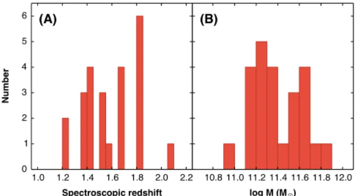
Figure 1(A) shows the redshift distribution of the sample. The mean and median redshifts are 1.56 and 1.59, respectively, with a standard deviation of 0.21. Virtually all objects belong to redshift spikes. Among the 24 objects, 14 have already been
Figure 1. Histograms of (A) the spectroscopic redshifts and (B) the stellar masses of the 24 galaxies in the sample.
published(Onodera et al.2010,2012) and the other 10 objects were identified during an observing run in 2011. We have removed 4 objects among the 18 identified in Onodera et al. (2012): object ID 313880 was removed because of the presence of Spitzer/MIPS 24μm emission, which may originate from star-forming activity or an AGN, and objects ID 209501, 253431, and 275414 were removed due to the lower confidence class for their spectroscopic redshifts.
2.2. Stellar Masses and Specific SFRs
We estimated stellar masses and SFRs by fitting synthetic spectral energy distributions to fluxes through broadbands extending from the u to the Spitzer/IRAC 8.5μm band and using the FAST code11(Kriek et al.2009) as described in detail in Onodera et al. (2012). In brief, we find a best-fit model within a grid of templates based on the 2007 version of Bruzal & Charlotʼs (2003) population synthesis models12adopting an exponentially declining SFH with various e-folding times τ. We allow for dust extinction adopting the extinction law by Calzetti et al.(2000). The Salpeter initial mass function (IMF; Salpeter 1955) was adopted, which may be appropriate for galaxies as massive as those in our sample (Shetty & Cappellari 2014). Age, mass, τ and metallicity are then the results of the procedure, having fixed the redshifts at the spectroscopic values. The resulting stellar masses13 are in the range 11<logM M<11.9, with a median of
M M
log =11.4 as shown in Figure1(B).
The MOIRCS spectra confirm the quenched nature of these galaxies, as they show no emission lines, a strong break at rest-frame 4000 Å, and strong absorption lines typical of old stellar populations. All objects have specific SFRs (sSFRºSFRM) below 10-11yr-1, as derived from the best-fit exponentially
declining SFH, which corresponds to a specific star formation rate(sSFR) of about two orders of magnitude lower than that of main-sequence galaxies at a similar redshift (e.g., Kashino et al.2013).
2.3. Structural Parameters
The effective radii, re, and Sérsic indices, n, of the 10
additional objects from the 2011 observing run were measured in exactly the same way as the rest of the sample presented in Onodera et al.(2012). In brief, we used GALFIT14version 3.0 (Peng et al.2002,2010a) to carry out a 2D Sérsic profile fitting for the images taken in the F814W filter with the Advanced Camera for Surveys on the Hubble Space Telescope (HST; Koekemoer et al.2007; Massey et al.2010). For each galaxy, we constructed the point-spread function (PSF) from nearby unsaturated stars. We estimated the sky background using three different methods:(1) the sky as a free parameter; (2) the sky fixed to the so-called pedestal GALFIT estimate; and (3) the sky manually measured from empty regions near the sample galaxy. We used the midpoints between the minimum and maximum of these runs, and half of the ranges as associated errors, for effective radius, Sérsic parameter, total magnitude, and axial ratio. GALFIT did not converge for objects 406178 and 531916 due to low surface brightness in the F814Wfilter.
Object IDs, coordinates, spectroscopic redshift, stellar mass, effective radius, and Sérsic index for all of the galaxies in the sample are listed in Table1.
2.4. Composite Spectrum
In order to achieve the high S/N needed for the measurement of the Lick indices, we constructed a composite spectrum by stacking the individual galaxy spectra in the same way as described in Onodera et al.(2012): all spectra were registered to the rest-frame wavelength by linearly interpolating on a 1 Å
interval, and normalized by the mean flux at
4500<l( )Å <5200 in the rest-frame. Noise spectra were also registered to the same rest-frame wavelength scale, but interpolated in quadrature. Then the spectra were co-added with weights proportional to the inverse square of the S/N at each wavelength pixel.
To correct for possible sampling bias, we computed the associated noise spectrum with the jackknife method as
(
)
N N f f 1 , (1) i N i Jack 2 1 ( ) 2å
s = - -=where N ( 24)= is the number of objects in the sample, f is the flux of the stacked spectrum of all N spectra, and f( )i is theflux
of a stacked spectrum made of N- spectra by removing the1 ith spectrum. We then corrected the stacked spectrum for the bias using
(
)(
)
f¢ = -f N-1 f( )i -f (2) where fi f N i N i ( ) 1 1 ( )á ñ = å = . The typical correction factor is very
small( 1%< ) in the wavelength range studied in this work, but it is a more realistic estimate of noise due to OH sky line residuals which vary significantly from pixel to pixel. We have adopted f′ andsJackas thefinal stacked spectrum and 1s noise
spectrum, respectively.
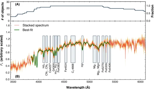
The resulting composite spectrum, corresponding to an equivalent integration time of about 200 hr on Subaru/ MOIRCS, is shown in Figure 2. This figure shows several clear absorption features, including the 4000 Å break, CaII H
+K lines, various Balmer absorption lines, the G-band, and Mg and Fe absorption features, which will be used in the next section to derive the stellar population parameters.
3. MEASUREMENT OF LICK ABSORPTION LINE INDICES
We measured the Lick indices on the stacked spectrum using LECTOR,15 following the definition given by Worthey & Ottaviani (1997) and Trager et al. (1998). We used the jackknife method to measure each index following Equations (1) and (2): we measured the indices on each f( )i and derived the bias-corrected index values and corresponding 1s error bars. The Lick indices measured on the stacked spectrum with the observed spectral resolution are listed in the second column in Table2.
11
http://astro.berkeley.edu/~mariska/FAST.html 12http://www.bruzual.org/cb07/
13
Sum of living stars and remnants. 14
Table 1
Properties of the Sample Galaxies
ID R.A. Decl. zspec logM M re Sérsic n
(deg) (deg) (kpc) 254025 150.6187115 2.0371363 1.8228± 0.0006 11.64-+0.030.15 3.16± 0.61 3.4± 0.4 217431 150.6646939 1.9497545 1.4277± 0.0015 11.82-+0.150.03 7.19± 1.95 3.8± 0.6 307881 150.6484873 2.1539903 1.4290± 0.0009 11.75 0.110.03 -+ 2.68± 0.12 2.3± 0.1 233838 150.6251048 1.9889180 1.8199± 0.0016 11.64-+0.250.16 2.25± 0.31 3.1± 0.3 277491 150.5833512 2.0890266 1.8163± 0.0038 11.56-+0.120.11 2.46± 0.11 1.0a 250093 150.6053729 2.0288998 1.8270± 0.0010 11.25-+0.080.13 3.00± 0.15 1.0a 263508 150.5677283 2.0594318 1.5212± 0.0009 11.11-+0.210.10 0.86± 0.03 3.2± 0.2 269286 150.5718552 2.0712204 1.6593± 0.0006 11.26-+0.280.02 1.03± 0.12 5.0± 0.7 240892 150.6432950 2.0073169 1.5494± 0.0009 11.29-+0.130.19 1.29± 0.13 3.0± 0.3 205612 150.6542714 1.9233323 1.6751± 0.0045 11.15-+0.060.13 2.08± 0.28 2.4± 0.3 251833 150.6293675 2.0336620 1.4258± 0.0006 10.99 0.050.27 -+ 1.61± 0.09 2.1± 0.1 228121 150.5936156 1.9754018 1.8084± 0.0015 11.39-+0.030.14 2.78± 0.86 4.1± 0.9 321998 150.7093826 2.1863891 1.5226± 0.0009 11.28-+0.090.12 1.83± 0.34 4.4± 0.6 299038 150.7091894 2.1369001 1.8196± 0.0010 11.30 0.150.08 -+ 0.96± 0.02 1.9± 0.0 519818 150.0124421 2.6406856 2.0879± 0.0010 11.37 0.240.28 -+ 1.69± 0.36 5.4± 0.7 526785 150.0057599 2.6548908 1.2454± 0.0383 11.44-+0.300.04 4.95± 0.54 3.1± 0.1 528213 150.0199418 2.6592730 1.3950± 0.0004 11.33-+0.220.32 3.06± 0.27 3.2± 0.2 535544 150.0027420 2.6748955 1.2452± 0.0003 11.68-+0.300.05 5.73± 1.22 4.2± 0.5 531916 149.9828887 2.6689945 1.3569± 0.0333 11.14-+0.410.28 K K 533754 150.0190505 2.6731339 1.3956± 0.0003 11.60-+0.180.04 2.42± 0.08 1.3± 0.1 543256 150.0179738 2.6948240 1.4340± 0.0008 11.29-+0.220.19 3.34± 0.39 3.7± 0.3 401700 150.2914647 2.3715033 1.6501± 0.0003 11.16-+0.140.25 1.73± 0.40 4.5± 1.0 411647 150.2915999 2.3956325 1.6525± 0.0008 11.56 0.310.08 -+ 2.67± 0.41 1.8± 0.3 406178 150.2881135 2.3813900 1.5718± 0.0037 11.56-+0.600.16 K K Notes. Effective radii are circularized, i.e., re=a q, where a and q are semimajor axis length and axis ratio, respectively.
a
The GALFIT run was carried out by fixing n = 1 (see Onodera et al.2012).
Figure 2. Composite rest-frame optical spectrum of the 24 quenched galaxies at z~1.6.(A): the number (left axis) and fraction (right axis) of spectra that have been stacked at each wavelength.(B): the stacked spectrum and associated 1σ error (orange solid line and filled region, respectively). The green solid line shows the best-fit combination of stellar spectra(Sánchez-Blázquez et al.2006b), using pPXF (Cappellari & Emsellem2004). The rectangles show the wavelength ranges used to measure the Lick indices of the stacked spectrum, though the Hβ index is not used in our stellar population analysis.
3.1. Broadening Measurement and Stellar Velocity Dispersion Measurements of Lick indices strongly depend on the broadening of the spectra: the larger the broadening, the shallower the absorption features and the more likely that part of the spectral feature falls outside the index windows. The total broadening (stot) is a combination of the intrinsic stellar
velocity dispersion (s) of the object, instrumental resolution
(sinstr), and stacking procedure reflecting redshift errors (sstack),
and can be expressed asstot2 =s2+sinstr2 +sstack2 (Cappellari et al. 2009). We measureds =tot 457 23 km s-1 by using the penalized pixel-fitting method (pPXF16; Cappellari & Emsellem2004) with template stellar spectra from the MILES database17 (Sánchez-Blázquez et al. 2006b). During the pPXF run, we masked wavelength ranges that are potentially contaminated by emission lines, namely Hγ, Hβ, and [OIII]
4959, 5007
ll . The best-fit combination of the templates is shown with the green solid line in Figure2.
Adopting the same procedure as Cappellari et al. (2009),
stack
s can be computed usingsstack» Dc z (1+ , where c isz) the speed of light andD is the redshift error. We computedz
stack
s for all objects used for stacking, and derived the average as sstack=10183km s-1 by using the bi-weight estimator (Beers et al.1990). Thissstackmay be a conservative estimate,
because objects with larger redshift errors have lower S/Ns and thus have less weight in the stacked spectrum. Adopting the instrumental resolution of sinstr=300 km s7 -1 (Onodera et al. 2010), by combining these numbers together, the stellar velocity dispersion of the stacked spectrum is estimated to be
330 41
s = km s-1. This is in good agreement with the average stellar velocity dispersion,ásinfñ = 29871km s-1, inferred from the structural parameters and stellar masses of the objects(Bezanson et al. 2011).
3.2. Broadening Correction
The resultings is in general larger than that of the originaltot
Lick/IDS system which is200–360 km s-1depending on the
indices. Therefore, the indices measured on our stacked spectrum have to be corrected to the Lick resolution. For this purpose, we computed the Lick indices on the MILES SSP models(Vazdekis et al.2010) by convolving the model spectra with the original Lick resolution (Worthey & Ottaviani1997; Schiavon 2007) and our resolution ofs =tot 460 km s-1. The MILES SSP models18 were constructed with a unimodal IMF with a slope of 1.3 (equivalent to the Salpeter IMF),
2.32 [M H] 0.22
- < < and age from 0.06 Gyr to that of the
universe at the corresponding redshift. We restricted the models to be in the safe range of parameters by setting Mode=SAFE. Comparing the indices measured with various broadenings, we found tight linear relations( 1% scatter) for all the indices and we used these relations to convert our values to those with the Lick/IDS resolution. The Lick indices corrected for the spectral resolution are listed in the third column in Table2.
4. STELLAR POPULATION PARAMETERS FROM LICK INDICES
In the following analysis we use a series of Lick indices for which synthetic models accurately reproduce those of Galactic globular clusters, as shown by Thomas et al.(2011b), namely: Hd , HA g , HA g , CNF 1, CN2, Ca4227, G4300, C24668, Mg1,
Mg2, Mgb, Fe4383, Fe4531, Fe5270, Fe5335, and Fe5406. The
Hβ index is widely used as an age indicator since it is less contaminated by metal lines, but it was not used in this analysis for the following two reasons. First, there may be a contribution from emission partially filling the absorption. Comparing the stacked spectra and best-fit template returned by pPXF, we measured a 3s upper limit of Å to the equivalent width of1 the Hβ emission line. On the other hand, the higher-order Balmer lines such as Hγ and Hδ are less affected by emission, with an equivalent width 0.5Å. Second, the Hβ indices in Galactic globular clusters are too weak for even the oldest SSP models to reproduce(Poole et al.2010). We would like to note, however, that the inclusion of Hβ to the set of indices above does not affect the results and conclusions presented here.
We derived the stellar population parameters, age,[Z/H], and [α/Fe], by comparing the Lick indices measured on the composite spectrum with those calculated from SSP models with variable abundance ratios19(Thomas et al. 2011b). Since the models give absolutefluxes by making use of flux-calibrated stellar spectral templates, the observed indices do not need to be converted to the Lick/IDS response. The models span the parameter space0.1<age Gyr<15,-2.25<[Z H]<0.67, and-0.3<[aFe]<0.5and adopt the Salpeter IMF.
For each index, we constructed a three-dimensional model grid of log(age), [Z/H], and [α/Fe] with an uniform interval of 0.025 dex for all three parameters and on this grid we computed the 2 index
(
Iindex I)
obs index model 2 index 2
å
c = - s , where Iindex obs and Iindexmodel are observed and model indices, respectively, andsindexis the1s error of the observed indices. Then we converted thec2
to a probability distribution p µexp
(
-c2 2)
, and normalized it such thatò
p d log(age)d[Z H]d[a Fe]= .1Table 2
Lick Indices Measured in the Stacked Spectrum
Index Raw Measurement Broadening Corrected HdA 4.27± 0.69 4.26± 0.72 HdF 3.26± 0.74 3.61± 0.79 CN1 −0.08 ± 0.02 −0.08 ± 0.02 CN2 −0.03 ± 0.03 −0.02 ± 0.03 Ca4227 −0.15 ± 0.48 −0.23 ± 0.75 G4300 4.45± 1.31 4.90± 1.34 HgA −0.88 ± 1.34 −0.95 ± 1.38 HgF 1.14± 0.73 1.38± 0.80 Fe4383 2.67± 1.38 3.57± 1.59 Fe4531 0.51± 1.12 0.70± 1.38 C24668 4.71± 1.09 5.51± 1.25 Hβ 2.36± 0.60 2.68± 0.73 Mg1 0.09± 0.02 0.10± 0.02 Mg2 0.18± 0.01 0.18± 0.01 Mgb 2.13± 0.72 2.88± 0.97 Fe5270 1.53± 0.89 2.09± 1.18 Fe5335 1.69± 0.71 3.25± 1.38 Fe5406 0.96± 1.05 1.88± 2.03 Note. CN1, CN2, Mg1, and Mg2indices are in a unit of magnitude; otherwise, indices are in a unit of Å. Hd and HF β indices are not used in the analysis presented in this work.
16 http://purl.org/cappellari/software 17 http://miles.iac.es/ 18 http://miles.iac.es/pages/webtools/tune-ssp-models.php 19 http://www.icg.port.ac.uk/~thomasd/tmj.html
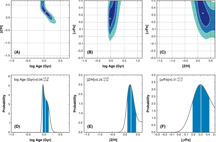
The resulting best-fit stellar population parameters are shown as white plus signs in Figure 3, which corresponds to the minimum reduced-c of2 ∼2.0. The reduced-c drops to 1.37 by2
removing the CN indices from the fit, while the best-fit parameters do not change at all. This poor fit due to the CN indices is not surprising, as nitrogen is not a free parameter in the fit (see also Thomas et al. 2011a, 2011b). Confidence regions enclosing 68.2%, 95.4%, and 99.7% of the total volume of the projected probability distributions are shown in the top panels of Figure 3. The probability distributions are marginalized to a one-dimensional parameter space (bottom panels in Figure 3) by adopting median values for each stellar population parameter and 16 and 84 percentiles as correspond-ing 1σ confidence intervals, respectively. In this way we have obtained log(age Gyr)=0.04-+0.080.10, [Z H]=0.24-+0.140.20, and
[ Fe] 0.31 0.12 0.12
a = -+ for the composite stellar population of our
24 galaxies. Of course, these uncertainties only reflect random errors associated with the measurement of the various indices and the quality of the fits, whereas systematic errors coming from the synthetic models may be significantly larger (e.g., Trager et al.2008).
5. DISCUSSION 5.1. Bias in the Sample
Spectroscopically identified samples could be biased toward relatively bluer, lower mass-to-light ratio objects, especially at
z>1.4, as pointed out by van de Sande et al. (2014). Although our sample is nearly complete down to KAB21.5 (Onodera et al. 2012), in this section we investigate potential biases that may affect our sample.
We computed rest-frame U-V and V-J colors of our sample and compared them with the photometric sample of passive BzK-selected galaxies in Figure 4. Since we have extracted the photometric sample for this comparison from a public catalog in the COSMOSfield by Muzzin et al. (2013a), we obtained the rest-frame colors using the Muzzin et al. photometry. We ran EAZY20(Brammer et al.2008) using the identical template set and input parameters as those used in Muzzin et al., except that redshifts are fixed to the spectro-scopic redshifts, and computed the rest-frame colors for U- and V-bands of Maíz Apellániz(2006) and 2MASS J-band. For the photometric sample extracted from the Muzzin et al. catalog, we required the photometry flag of unity, non-detection in Spitzer/MIPS 24μm, and KAB<21.5to match the selection of our sample, in addition to the standard passive BzK selection criteria(Daddi et al.2004).
Figure4shows that the majority of our sample are classified as “old quenched” according to the Whitaker et al. (2012a) criterion and the overall distribution appears to be consistent with that of the parent sample. Quantitatively, the median
colors of our sample and the parent sample are
V J U V
( - , - )=(1.16, 1.78)and V( -J U, -V)=(1.10, 1.85),
Figure 3. Probability distributions of stellar population parameters for the quenched galaxies at z~1.6. Top: two-dimensional probability distributions in the(A) age–[Z/H], (B) age–[α/Fe], and (C) [Z/H]–[α/Fe] planes. Cross symbols show the peak of the probability distributions and the contours indicate the areas that enclose 68.2%, 95.4%, and 99.7% of the probability distributions, respectively. Bottom: one-dimensional probability distributions for(D) age, (E) [Z/H], and (F) [α/Fe]. The vertical white solid lines indicate the median values, and the left and right edges of thefilled regions define the 16 and 84 percentiles, respectively.
20
respectively. Note that the typical uncertainty in the rest-frame colors is 0.1–0.2 mag (e.g., Williams et al.2009) and the above differences are consistent within it. One might argue that the UVJ selection cannot perfectly isolate the passive BzK population in the quiescent section of the diagram or vice versa, even though there appears to be no signature of emission lines in our spectroscopic sample. However, we would like to note that both UVJ and BzK diagnostics select quenched galaxies only in a statistical sense and some degree of contamination outside of the quiescent region is not entirely unexpected(see Moresco et al.2013for a detailed comparison of various selection methods of passive galaxies at z<1).
Whitaker et al. (2013) have derived stellar population ages of UVJ-selected quiescent galaxies at1.4< <z 2.2identified in HST/WFC3 G141 grism observations from the 3D-HST survey(Brammer et al. 2012). The average age is 1.3-+0.30.1Gyr
for all quiescent galaxies, which is in excellent agreement with that of our quenched galaxies at similar redshift. They also split the sample into young and old quiescent galaxies, and the derived ages for both classes are consistent with ours within the uncertainties.
Comparisons of the rest-frame colors with the parent passive BzK sample and of the stellar population ages with the galaxies with similar colors from Whitaker et al.(2013) suggest that our spectroscopic sample is not likely to be biased toward younger ages and appears to be representative of the quenched galaxy population at zá ñ =1.6. However, the comparison discussed here is based on the K-selected sample. Therefore, the lack of apparent bias in our spectroscopic sample with respect to the photometric one does not necessarily mean that there is no bias compared to the entire (e.g., mass-selected) quiescent population.
5.2. Redshift Evolution of Stellar Populations in Quenched Galaxies
Figure 5 compares the stellar population luminosity-weighted age, [Z/H], and [α/Fe] of various sets of quenched galaxies at different redshifts. Having derived an age log(age Gyr) 0.04 0.08
0.10
= -+ , or 1.1Gyr, from the composite
spectrum, we calculate that the passive aging over ∼9.5 Gyr from zá ñ =1.6to z= 0, i.e., to an age of ∼11 Gyr, will bring the stellar populations of these galaxies to the point indicated by the arrowhead in Figure5(A). This is in excellent agreement with the luminosity-weighted ages of stellar populations in local quenched galaxies of similar velocity dispersions by Spolaor et al. (2010), who derive the stellar population parameters via Lick indices using stellar population models from Thomas et al.(2003), which are equivalent in this respect to the Thomas et al.(2011b) models adopted in this study.
Figure 5(B) shows the age–redshift relations for different values of the formation redshift zf (gray solid lines), assuming
a single burst of star formation at zf. In this SSP approximation,
the average age of∼1.1 Gyr indicates a formation redshift of z
2 f 2.5for the bulk of the stars. Figure5(B) also shows the stellar population ages of similarly massive, quenched galaxies in clusters at z=0.54, 0.83, and 0.89(Jørgensen & Chiboucas 2013). These are currently the only ages for quenched galaxies at these intermediate epochs with compar-ableσ that have been derived in a homogeneous way similar to our galaxies, i.e., using the Lick indices and the Thomas et al. (2011b) models to derive the stellar population parameters. Apart from a possible(small) bias due to the special location in high density peaks, these lower redshift cluster galaxies fit remarkably well along the evolutionary trend expected for pure passive evolution from zá ñ = 1.6to z= 0.
Furthermore, Figure 5 shows that the derived metallicity [Z H] 0.24 0.14
0.20
= -+ , or 1.7Z, of our composite zá ñ =1.6
galaxies is the same as that of local quenched galaxies of similar velocity dispersion (Spolaor et al. 2010). The two different colors—blue and orange—in the figure correspond to the values measured at the central part of galaxies(within re/8)
and within the effective radius, respectively. The aperture used to extract the spectra of the zá ñ =1.6sample is about (2– r3) e.
In the case that the galaxy is well resolved, stellar population parameters derived within large radii(e.g., r>re) converge to
those integrated to the effective radius (Kobayashi & Arimoto 1999). However, our sample was observed with an FWHM of the PSF corresponding to . van de Sande et al.2re
(2013) have examined the aperture correction for velocity dispersion measurements by taking PSF and aperture effects into account for a Sérsic profile and we have followed the same approach to investigate these effects on the derived metallicity. Since radial metallicity gradients in the local quenched galaxies are very steep(D[Z H]Dlogr= -0.23; Spolaor et al.2010, see also Kuntschner et al.2010; Koleva et al.2011), the change in[Z/H] integrated within r 8e and out to rreis found to be
only0.05dex when coupled with a Sérsic profile with n1 and large PSF size compared to the effective radius. Therefore, our measured [Z/H] appears to be more representative of the central value. Note that the measured indices, hence the derived age, [Z/H], and [α/Fe] presented in Jørgensen & Chiboucas (2013) for intermediate-z cluster galaxies have already been corrected to the values within 3.4 arcsec at the distance of the Coma cluster, based on measurements of index gradients of
Figure 4. Rest-frame UVJ color–color diagram. Red circles are our quenched galaxies at zá ñ =1.6with UVJ colors computed as described in Section5.1. Gray dots represent photometrically selected passive BzK galaxies (Daddi et al.2004) with reliable photometry, non-detection in Spitzer/MIPS 24 μm, and KAB<21.5taken from Muzzin et al.(2013a). Blue and red areas indicate regions to separate young and old quiescent galaxies, respectively, while the rest of the diagram classifies galaxies as star-forming (Whitaker et al.2012a).
local galaxies (Jørgensen & Chiboucas 2013, see also Jørgensen et al. 1995; Jørgensen et al. 2005).
The α-to-iron abundance ratio measured for the zá ñ =1.6 quenched galaxies, [ Fe] 0.31 0.12
0.12
a = -+ , or∼2 times the solar
value, lies precisely on the z= 0 [α/Fe]–σ relation (Figure5; e.g., Kuntschner et al.2010; Spolaor et al.2010; Thomas et al. 2010), indicating little or no evolution at a given velocity dispersion of the [α/Fe] ratio over the past ∼10 Gyr.
Thus, it appears that the chemical composition is indeed frozen in during passive evolution from zá ñ =1.6 to 0. We conclude
that the stellar population content, i.e., their age, metallicity and α-element enhancement of our zá ñ =1.6galaxies, qualifies them as possible progenitors of similarly massive quenched galaxies at z= 0, from purely passive evolution.
5.3. SFHs of Quenched Galaxies at zá ñ =1.6 and Their Precursors
We turn now to the other side in cosmic times, i.e., toward higher redshifts and earlier epochs, trying to identify possible
Figure 5. Stellar population parameters as a function of stellar velocity dispersion (A), (C), (E), and redshift (B), (D), (F). Shown are the luminosity-weighted age (A), (B), [Z/H] (C), (D), and the [α/Fe] ratio (E), (F) of stellar populations in quenched galaxies at various redshifts. In each panel, the red symbol represents our measurement at zá ñ =1.6. In the right panels, the thick and thin error bars correspond to the standard deviation and range of redshift of the sample, respectively. Blue and orange symbols show z= 0 values within r 8e and re, respectively, of local quenched galaxies(Spolaor et al.2010). In the right panels, blue and orange points are the corresponding median properties of the local sample withs >200km s-1with the 1σ scatter of the corresponding distribution. The red arrowhead in panel (A) shows the ending point of a purely passive evolution of the stellar populations of our sample galaxies down to z= 0. Gray circles in the right panels show the values for massive quenched galaxies with logs( km s )-1 >2.24in intermediate redshift clusters (Jørgensen & Chiboucas2013). Their measurements were aperture corrected in order to match the nuclear measurements at z= 0. In panel (B), the gray solid lines show, from thin to thick, the age of simple stellar populations made at a formation redshifts from 1.5 to 4.0, as indicated in the insert.
progenitors of our quenched galaxies at zá ñ = 1.6. At higher redshift star-forming galaxies dominate the massive galaxy population(e.g., Ilbert et al.2013; Muzzin et al.2013b) and it is among them that precursors should be sought. The average age∼1.1 Gyr of our quenched galaxies at zá ñ =1.6indicates a formation redshift of zf 2.3for their stellar populations, as also indicated in Figure 5(B). As already mentioned, having been derived from fits to SSPs, this “age” is essentially a measure of the time elapsed since their star formation was quenched. Indeed, if the SFR was rapidly increasing, as expected for the evolution of main-sequence galaxies at such high redshift (Renzini 2009; Peng et al. 2010b), then the corresponding formation redshift must also be close to the quenching epoch, as most of the stars formed just prior to the quenching. By the same token, these authors argue that an α-element enhancement relative to the solar abundance ratio is the natural outcome of such a (quasi-exponential) rapid increase in SFR.
Following Thomas et al.(2005), we use the measured [α/Fe] ratio to estimate the star formation timescale of the precursors
as log( t Gyr) 6 1
5 [aFe]
D » ´æ
è
ççç - öø÷÷÷= 0.66 0.72- . Given the large error bars and the approximate nature of this relation, we conservatively adopt a1s upper limit ofD Gyr, andt 1
translate this timescale into a specific SFR
M t
(sSFRºSFR )=1 D 1 Gyr-1. At the median stellar
mass of our sample, the corresponding lower limit for the SFR just prior to the quenching is therefore SFR200M yr-1
.
This matches the measured SFR of main-sequence star-forming galaxies of similar stellar mass at z2 (e.g., Daddi et al.2007; Pannella et al.2015; Rodighiero et al.2014).
As an independent consistency check we have adopted an exponentially rising SFR as appropriate for star-forming main-sequence galaxies at z ~2 (e.g., Renzini 2009; Maraston et al.2010; Papovich et al.2011; Reddy et al.2012) and have estimated that a SFR culminating at~300M yr-1
just prior to
the quenching would be required to build a stellar mass of M
2.3´1011 by z=2.3, i.e., at the average quenching epoch
and mass for our sample. Again, this is in good agreement with the pre-quenching SFR that we have inferred from the [α/Fe] ratio.
Detailed studies of massive, M >1011M
star-forming
main-sequence galaxies at z >2–2.5 with resolved kpc-scale gas kinematics, SFR and stellar mass densities, and emission line profiles secured in recent years (Förster Schreiber et al. 2009, and N. M. Förster Schreiber et al. 2015, in preparation; Tacchella et al.2015b) show that their high SFRs are mostly sustained at high galactocentric distances (Genzel et al. 2014b; Tacchella et al. 2015a). By contrast, the central regions of such galaxies are already relatively quenched, and have reached central mass concentrations that are similar to those of z = 0 quenched spheroids (Tacchella et al. 2015a). These inner quenched spheroidal components argue for an inside-out quenching process, as expected, for example, in the case of AGN feedback or gravitational quenching (but see Sargent et al. 2015). Moreover, these galaxies show strong nuclear outflows running at up to 1600 km s~ -1, which are
most likely driven by AGN feedback (Cimatti et al. 2013; Förster Schreiber et al. 2014; Genzel et al. 2014a). These outflows provide tantalizing support for AGN-related processes being responsible for quenching, though evidence for AGN feedback is not necessarily evidence for AGN quenching.
These z2 galaxies qualify as possible precursors to our quenched galaxies at z~1.6for two reasons. First, all z~2.3 massive galaxies on the main sequence must soon be quenched, otherwise they would dramatically overgrow (Renzini 2009; Peng et al.2010b). Second, their properties (described above) indicate that the quenching process may already be under way. These observations seem to support the notion that mass quenching of star formation in massive galaxies (Peng et al. 2010b) is predominantly a rapid process, as opposed to an slow quenching process such as halo quenching (Woo et al.2015, but see Knobel et al.2015).
5.4. Size Growth and Progenitor Bias
As we showed above, a purely passive evolution of our quenched galaxies to z~ , i.e., without any further star0 formation, will bring their stellar population properties to closely match their counterparts in the local universe. However, quenched galaxies at high redshifts are known to have smaller sizes compared to local galaxies (e.g., Daddi et al. 2005; Trujillo et al. 2006; Cimatti et al. 2008; van Dokkum et al. 2008; Cassata et al. 2011; van der Wel et al. 2014). The average effective radius of 2.7 kpc that we have measured for the 24 zá ñ =1.6galaxies is, indeed, a factor of∼2.5 smaller than that of local quenched galaxies of the same stellar mass (Table1; Newman et al.2012). Two main processes have been suggested and extensively discussed as being responsible for the average size growth of the quenched galaxy population: the growth of individual galaxies and the addition of larger-sized quenched galaxies at later epochs (Carollo et al. 2013). A series of minor dry mergers with other quenched galaxies is one effective way to increase the sizes of individual galaxies, by adding an extended envelope to a pre-existing compact galaxy (e.g., Hopkins et al.2009; Naab et al.2009; Cappellari2013). Based on the study of abundance ratios of different elements, Greene et al.(2012,2013) found that stellar populations in the outskirts ( r ) of nearby massive early-type galaxies2e
(s 150 km s-1
) are different from those in the inner
regions, as they are composed of similarly old (∼10 Gyr) but more metal-poor ([Fe H]~ -0.5) and α-element enhanced ([ Fe]a ~0.3) stars. They argue that these distinct stellar populations have formed at z>1.5–2 in less massive systems and then accreted onto the outskirts of massive quenched galaxies. This scenario is consistent with our results, as the stellar population parameters of both low and high-redshift galaxies considered here were measured essentially within the central part of the galaxies.
One problem with this mechanism for growing galaxies is that it requires minor merging events to be gas-poor, otherwise gas would sink to the bottom of the potential well, leading to further star formation and resulting in an even more compact galaxy(Naab et al.2009). However, at z1.5most galaxies appear to be gas-rich and forming stars(e.g., Daddi et al.2010; Tacconi et al.2010,2013; Sargent et al. 2014), and it seems rather difficult for massive quenched galaxies to accrete selectively quenched galaxies and avoid gas accretion and subsequent star formation. Still, one may speculate that galactic conformity, the phenomenon that satellites of quenched centrals are more likely to be quenched even out to z (e.g., Weinmann et al.2 2006; Hartley et al.2015; Knobel et al.2015), might help make small systems quiescent before they are accreted. Moreover, Williams et al. (2011) and Newman et al. (2012) do not find a sufficient number of
satellites around massive quenched galaxies to account for their size growth between z= 2 and 1.
Thus an alternative or additional process to secularly grow the average size of quenched galaxies needs to be considered. At stellar masses1011M, the number density of quenched
galaxies increases by about one order of magnitude between z= 2 and z = 0 (e.g., Cassata et al.2013; Muzzin et al.2013b), with most of the increase for massive galaxies having taken place by z ~1 (e.g., Cimatti et al. 2006). Thus, it has been argued that at least part of the evolution in the average size of quenched galaxies should be due to the continuous addition of quenched galaxies that are already larger than those formed at earlier times (e.g., Carollo et al.2013; Poggianti et al. 2013). Indeed, the average size of star-forming galaxies also increases with time, running above and nearly parallel to the average size of quenched galaxies (van der Wel et al. 2014). Therefore, newly quenched galaxies are likely to be larger than pre-existing ones and also smaller than the star-forming progenitors due to the fast fading of the quenched disk (Carollo et al. 2014). This effect, a kind of progenitor bias, could explain some of the apparent size evolution of quenched galaxy populations, given the mentioned difficulties of the scenario invoking the size growth of individual galaxies, though the two effects are also likely to work together(Belli et al.2015).
For these reasons, a comparison between galaxy populations at different redshifts andfixed stellar masses could suffer from this progenitor bias. However, Bezanson et al.(2012) showed that the number density of quiescent galaxies with large sinf
( 250 km s -1) is remarkably constant at0.3< <z 1.5, which
indicates that the build-up of quiescent galaxy populations with high velocity dispersions was largely completed by z~1.5. Thus, a comparison based on stellar velocity dispersions could greatly reduce the effect of the progenitor bias. Indeed, in Figure 5 essentially all of the nearby early-type galaxies presented in Spolaor et al.(2010) withs > 250 km s−1have stellar population ages 10Gyr. The age distribution of morphologically selected SDSS early-type galaxies with
250
s km s−1 at0.05< <z 0.06 also peaks at an age of
10 Gyr (Thomas et al. 2010), which is in good agreement with the expected age for our zá ñ =1.6sample assuming pure passive evolution down to z~0.05.
6. SUMMARY
Using a rest-frame optical composite spectrum of 24 massive quenched galaxies at zá ñ =1.6and with Má ñ =2.5´1011M
,
we have derived luminosity-weighted stellar population para-meters from Lick absorption line indices, namely age,[Z/H], and [α/Fe], and have discussed their past SFH and subsequent evolution toward lower redshifts, identifying the likely progeni-tors and descendants of similar galaxies. Our main results can be summarized as follows.
1. The average stellar population properties derived are log(age Gyr)=0.04-+0.080.10, or ∼1.1 Gyr, [Z H]=0.24-+0.140.20,
and [ Fe] 0.31 0.12 0.12
a = -+ . The average stellar velocity
dispersion of these galaxies is s = 33041km s-1, as measured from the composite spectrum.
2. The á ñ =z 1.6 galaxies show [Z/H] and [α/Fe] in excellent agreement with those of local early-type galaxies at similar velocity dispersions. Pure passive evolution to z = 0 brings the age of these zá ñ =1.6 quenched galaxies to coincide with that of their local
counterparts at the same s. Therefore, the stellar
populations of the galaxies in our sample qualify such galaxies as plausible progenitors of similarly massive quenched galaxies in the local universe.
3. The age of 1.1 Gyr for the bulk of stars in these galaxies points to a formation redshift of zf ~2.3, an epoch when massive galaxies on the main sequence are very rapidly growing in mass and therefore must soon be quenched. 4. The[α/Fe] value indicates a star formation timescale of
t1
D Gyr which in turn implies a typical SFR of
M
200 yr 1
~
- just prior to the quenching. This SFR is
well within a range covered by similarly massive main-sequence galaxies at z~2.3.
5. These properties of massive z~2.3 main-sequence galaxies qualify them as likely precursors to our quenched galaxy at zá ñ =1.6.
One limitation of the present study is that we had to stack individual spectra to an equivalent integration time of∼200 hr in order to achieve a high S/N that was adequate for the analysis of the Lick indices. Further studies based on high S/N spectra of individual galaxies are needed to account for a diversity in high-redshift quenched galaxy populations (e.g., Belli et al. 2015). This is becoming possible through deep absorption line spectroscopy with the new generation of near-IR spectrographs such as Keck/MOSFnear-IRE and VLT/KMOS, though very long integration times will still be necessary.
We are grateful to the referee for useful and constructive comments. We thank the staff of the Subaru telescope, especially Ichi Tanaka, for supporting the observations. We also thank Sumire Tatehora, Will Hartley, Claudia Maraston, Daniel Thomas, and Alexandre Vazdekis for fruitful discus-sions, and Joanna Woo for reading the manuscript thoughtfully. We acknowledge Inger Jørgensen for providing us with measurements in electronic form. This work has been partially supported by the Grant-in-aid for the Scientific Research Fund under grant No. 23224005, and the Program for Leading Graduate Schools PhD Professional: Gateway to Success in Frontier Asia, commissioned by the Ministry of Education, Culture, Sports, Science and Technology (MEXT) of Japan. This research made extensive use of Astropy,21 a commu-nity-developed core Python package for Astronomy (Astropy Collaboration et al.2013), and matplotlib,22a Python 2D plotting library(Hunter2007).
Facilities: Subaru(MOIRCS)
REFERENCES
Astropy Collaboration, Robitaille, T. P., Tollerud, E. J., et al. 2013, A&A, 558, A33
Bedregal, A. G., Scarlata, C., Henry, A. L., et al. 2013,ApJ,778, 126 Beers, T. C., Flynn, K., & Gebhardt, K. 1990,AJ,100, 32
Belli, S., Newman, A. B., & Ellis, R. S. 2014a,ApJ,783, 117 Belli, S., Newman, A. B., & Ellis, R. S. 2015,ApJ,799, 206
Belli, S., Newman, A. B., Ellis, R. S., & Konidaris, N. P. 2014b,ApJL,788, L29 Bezanson, R., van Dokkum, P., & Franx, M. 2012,ApJ,760, 62
Bezanson, R., van Dokkum, P., van de Sande, J., Franx, M., & Kriek, M. 2013, ApJL,764, L8
Bezanson, R., van Dokkum, P. G., Franx, M., et al. 2011,ApJL,737, L31 Birnboim, Y., & Dekel, A. 2003,MNRAS,345, 349
Bouché, N., Dekel, A., Genzel, R., et al. 2010,ApJ,718, 1001 21
http://www.astropy.org 22
Brammer, G. B., van Dokkum, P. G., & Coppi, P. 2008,ApJ,686, 1503 Brammer, G. B., van Dokkum, P. G., Franx, M., et al. 2012,ApJS,200, 13 Brinchmann, J., Charlot, S., White, S. D. M., et al. 2004,MNRAS,351, 1151 Bruzual, G., & Charlot, S. 2003,MNRAS,344, 1000
Burstein, D., Faber, S. M., Gaskell, C. M., & Krumm, N. 1984,ApJ,287, 586 Calzetti, D., Armus, L., Bohlin, R. C., et al. 2000,ApJ,533, 682
Cappellari, M. 2013,ApJL,778, L2
Cappellari, M., & Emsellem, E. 2004,PASP,116, 138
Cappellari, M., di Serego Alighieri, S., Cimatti, A., et al. 2009,ApJL,704, L34 Carollo, C. M., Bschorr, T. J., Renzini, A., et al. 2013,ApJ,773, 112 Carollo, C. M., Cibinel, A., Lilly, S. J., et al. 2014, arXiv:1402.1172 Carollo, C. M., Danziger, I. J., & Buson, L. 1993,MNRAS,265, 553 Cassata, P., Giavalisco, M., Guo, Y., et al. 2011,ApJ,743, 96 Cassata, P., Giavalisco, M., Williams, C. C., et al. 2013,ApJ,775, 106 Choi, J., Conroy, C., Moustakas, J., et al. 2014,ApJ,792, 95 Cimatti, A., Brusa, M., Talia, M., et al. 2013,ApJL,779, L13 Cimatti, A., Cassata, P., Pozzetti, L., et al. 2008,A&A,482, 21 Cimatti, A., Daddi, E., & Renzini, A. 2006,A&A,453, L29 Cimatti, A., Daddi, E., Renzini, A., et al. 2004,Natur,430, 184 Conroy, C., Graves, G. J., & van Dokkum, P. G. 2014,ApJ,780, 33 Croton, D. J., Springel, V., White, S. D. M., et al. 2006,MNRAS,365, 11 Daddi, E., Bournaud, F., Walter, F., et al. 2010,ApJ,713, 686
Daddi, E., Cimatti, A., Renzini, A., et al. 2004,ApJ,617, 746 Daddi, E., Dickinson, M., Morrison, G., et al. 2007,ApJ,670, 156 Daddi, E., Renzini, A., Pirzkal, N., et al. 2005,ApJ,626, 680 Davé, R., Finlator, K., & Oppenheimer, B. D. 2012, MNRAS,421, 98 Dekel, A., Birnboim, Y., Engel, G., et al. 2009,Natur,457, 451 Elbaz, D., Daddi, E., Le Borgne, D., et al. 2007,A&A,468, 33
Förster Schreiber, N. M., Genzel, R., Bouché, N., et al. 2009,ApJ,706, 1364 Förster Schreiber, N. M., Genzel, R., Newman, S. F., et al. 2014,ApJ,787, 38 Gallazzi, A., Bell, E. F., Zibetti, S., Brinchmann, J., & Kelson, D. D. 2014,
ApJ,788, 72
Genzel, R., Förster Schreiber, N. M., Lang, P., et al. 2014b,ApJ,785, 75 Genzel, R., Förster Schreiber, N. M., Rosario, D., et al. 2014a,ApJ,796, 7 Glazebrook, K., Abraham, R. G., McCarthy, P. J., et al. 2004,Natur,430, 181 Gobat, R., Strazzullo, V., Daddi, E., et al. 2012,ApJL,759, L44
Gobat, R., Strazzullo, V., Daddi, E., et al. 2013,ApJ,776, 9
Greene, J. E., Murphy, J. D., Comerford, J. M., Gebhardt, K., & Adams, J. J. 2012,ApJ,750, 32
Greene, J. E., Murphy, J. D., Graves, G. J., et al. 2013,ApJ,776, 64 Hartley, W. G., Conselice, C. J., Mortlock, A., Foucaud, S., & Simpson, C.
2015,MNRAS,451, 1613
Hopkins, P. F., Hernquist, L., Cox, T. J., et al. 2006,ApJS,163, 1 Hopkins, P. F., Hernquist, L., Cox, T. J., Keres, D., & Wuyts, S. 2009,ApJ,
691, 1424
Hunter, J. D. 2007, CSE,9, 90
Ichikawa, T., Suzuki, R., Tokoku, C., et al. 2006,Proc. SPIE,6269, 16 Ilbert, O., McCracken, H. J., Le Fèvre, O., et al. 2013,A&A,556, A55 Jørgensen, I., Bergmann, M., Davies, R., et al. 2005,AJ,129, 1249 Jørgensen, I., & Chiboucas, K. 2013,AJ,145, 77
Jørgensen, I., Franx, M., & Kjaergaard, P. 1995, MNRAS,276, 1341 Karim, A., Schinnerer, E., Martínez-Sansigre, A., et al. 2011,ApJ,730, 61 Kashino, D., Silverman, J. D., Rodighiero, G., et al. 2013,ApJL,777, L8 Kelson, D. D. 2014, arXiv:1406.5191
Kelson, D. D., Illingworth, G. D., Franx, M., & van Dokkum, P. G. 2001, ApJL,552, L17
Kelson, D. D., Illingworth, G. D., Franx, M., & van Dokkum, P. G. 2006,ApJ, 653, 159
Knobel, C., Lilly, S. J., Woo, J., & Kovač, K. 2015,ApJ,800, 24 Kobayashi, C., & Arimoto, N. 1999,ApJ,527, 573
Koekemoer, A. M., Aussel, H., Calzetti, D., et al. 2007,ApJS,172, 196 Koleva, M., Prugniel, P., de Rijcke, S., & Zeilinger, W. W. 2011,MNRAS,
417, 1643
Kriek, M., van Dokkum, P. G., Franx, M., et al. 2008,ApJ,677, 219 Kriek, M., van Dokkum, P. G., Labbé, I., et al. 2009,ApJ,700, 221 Krogager, J.-K., Zirm, A. W., Toft, S., Man, A., & Brammer, G. 2014,ApJ,
797, 17
Kuntschner, H., Emsellem, E., Bacon, R., et al. 2010,MNRAS,408, 97 Lilly, S. J., Carollo, C. M., Pipino, A., Renzini, A., & Peng, Y. 2013,ApJ,
772, 119
Magdis, G. E., Rigopoulou, D., Huang, J.-S., & Fazio, G. G. 2010,MNRAS, 401, 1521
Maíz Apellániz, J. 2006,AJ,131, 1184
Maraston, C., Pforr, J., Renzini, A., et al. 2010,MNRAS,407, 830 Martig, M., Bournaud, F., Teyssier, R., & Dekel, A. 2009,ApJ,707, 250
Massey, R., Stoughton, C., Leauthaud, A., et al. 2010,MNRAS,401, 371 Matteucci, F., & Greggio, L. 1986, A&A,154, 279
McCracken, H. J., Capak, P., Salvato, M., et al. 2010,ApJ,708, 202 Moresco, M., Pozzetti, L., Cimatti, A., et al. 2013,A&A,558, A61 Muzzin, A., Marchesini, D., Stefanon, M., et al. 2013a,ApJS,206, 8 Muzzin, A., Marchesini, D., Stefanon, M., et al. 2013b,ApJ,777, 18 Naab, T., Johansson, P. H., & Ostriker, J. P. 2009,ApJL,699, L178 Newman, A. B., Ellis, R. S., Bundy, K., & Treu, T. 2012,ApJ,746, 162 Noeske, K. G., Weiner, B. J., Faber, S. M., et al. 2007,ApJL,660, L43 Oke, J. B., & Gunn, J. E. 1983,ApJ,266, 713
Onodera, M., Daddi, E., Gobat, R., et al. 2010,ApJL,715, L6 Onodera, M., Renzini, A., Carollo, M., et al. 2012,ApJ,755, 26 Pannella, M., Carilli, C. L., Daddi, E., et al. 2009,ApJL,698, L116 Pannella, M., Elbaz, D., Daddi, E., et al. 2015,ApJ,807, 141
Papovich, C., Finkelstein, S. L., Ferguson, H. C., Lotz, J. M., & Giavalisco, M. 2011, MNRAS,412, 1123
Peng, C. Y., Ho, L. C., Impey, C. D., & Rix, H.-W. 2002,AJ,124, 266 Peng, C. Y., Ho, L. C., Impey, C. D., & Rix, H.-W. 2010a,AJ,139, 2097 Peng, Y.-j., Lilly, S. J., Kovač, K., et al. 2010b,ApJ,721, 193
Poggianti, B. M., Moretti, A., Calvi, R., et al. 2013,ApJ,777, 125 Poole, V., Worthey, G., Lee, H.-c., & Serven, J. 2010,AJ,139, 809 Reddy, N. A., Pettini, M., Steidel, C. C., et al. 2012,ApJ,754, 25 Renzini, A. 2009,MNRAS,398, L58
Rodighiero, G., Daddi, E., Baronchelli, I., et al. 2011,ApJL,739, L40 Rodighiero, G., Renzini, A., Daddi, E., et al. 2014,MNRAS,443, 19 Salmi, F., Daddi, E., Elbaz, D., et al. 2012,ApJL,754, L14 Salpeter, E. E. 1955,ApJ,121, 161
Sánchez-Blázquez, P., Gorgas, J., Cardiel, N., & González, J. J. 2006a,A&A, 457, 809
Sánchez-Blázquez, P., Peletier, R. F., Jiménez-Vicente, J., et al. 2006b, MNRAS,371, 703
Sargent, M. T., Daddi, E., Béthermin, M., et al. 2014,ApJ,793, 19 Sargent, M. T., Daddi, E., & Bournard, F. 2015,ApJL,806, L20 Schiavon, R. P. 2007,ApJS,171, 146
Scoville, N., Aussel, H., Brusa, M., et al. 2007,ApJS,172, 1 Shetty, S., & Cappellari, M. 2014,ApJL,786, L10
Speagle, J. S., Steinhardt, C. L., Capak, P. L., & Silverman, J. D. 2014,ApJS, 214, 15
Spolaor, M., Kobayashi, C., Forbes, D. A., Couch, W. J., & Hau, G. K. T. 2010,MNRAS,408, 272
Suzuki, R., Tokoku, C., Ichikawa, T., et al. 2008, PASJ,60, 1347 Tacchella, S., Carollo, C. M., Renzini, A., et al. 2015a,Sci,348, 314 Tacchella, S., Lang, P., Carollo, C. M., et al. 2015b,ApJ,802, 101 Tacconi, L. J., Genzel, R., Neri, R., et al. 2010,Natur,463, 781 Tacconi, L. J., Neri, R., Genzel, R., et al. 2013,ApJ,768, 74 Thomas, D., Greggio, L., & Bender, R. 1999,MNRAS,302, 537 Thomas, D., Johansson, J., & Maraston, C. 2011a,MNRAS,412, 2199 Thomas, D., Maraston, C., & Bender, R. 2003,MNRAS,339, 897 Thomas, D., Maraston, C., Bender, R., & Mendes de Oliveira, C. 2005,ApJ,
621, 673
Thomas, D., Maraston, C., & Johansson, J. 2011b,MNRAS,412, 2183 Thomas, D., Maraston, C., Schawinski, K., Sarzi, M., & Silk, J. 2010,
MNRAS,404, 1775
Toft, S., Gallazzi, A., Zirm, A., et al. 2012,ApJ,754, 3
Trager, S. C., Faber, S. M., & Dressler, A. 2008,MNRAS,386, 715 Trager, S. C., Faber, S. M., Worthey, G., & González, J. J. 2000, AJ,
119, 1645
Trager, S. C., Worthey, G., Faber, S. M., Burstein, D., & Gonzalez, J. J. 1998, ApJS,116, 1
Trujillo, I., Förster Schreiber, N. M., Rudnick, G., et al. 2006,ApJ,650, 18 van de Sande, J., Kriek, M., Franx, M., Bezanson, R., & van Dokkum, P. G.
2014,ApJL,793, L31
van de Sande, J., Kriek, M., Franx, M., et al. 2011,ApJL,736, L9 van de Sande, J., Kriek, M., Franx, M., et al. 2013,ApJ,771, 85 van der Wel, A., Franx, M., van Dokkum, P. G., et al. 2014,ApJ,788, 28 van Dokkum, P. G., Franx, M., Kriek, M., et al. 2008,ApJL,677, L5 Vazdekis, A., Sánchez-Blázquez, P., Falcón-Barroso, J., et al. 2010, MNRAS,
404, 1639
Weinmann, S. M., van den Bosch, F. C., Yang, X., & Mo, H. J. 2006, MNRAS,366, 2
Whitaker, K. E., Kriek, M., van Dokkum, P. G., et al. 2012a,ApJ,745, 179 Whitaker, K. E., van Dokkum, P. G., Brammer, G., & Franx, M. 2012b,ApJL,
754, L29
Whitaker, K. E., Franx, M., Leja, J., et al. 2014,ApJ,795, 104
Williams, R. J., Quadri, R. F., & Franx, M. 2011,ApJL,738, L25
Williams, R. J., Quadri, R. F., Franx, M., van Dokkum, P., & Labbé, I. 2009, ApJ,691, 1879
Woo, J., Dekel, A., Faber, S. M., & Koo, D. C. 2015,MNRAS,448, 237
Worthey, G., Faber, S. M., Gonzalez, J. J., & Burstein, D. 1994,ApJS,94, 687 Worthey, G., & Ottaviani, D. L. 1997,ApJS,111, 377
Yamada, Y., Arimoto, N., Vazdekis, A., & Peletier, R. F. 2006,ApJ,637, 200 Yoshikawa, T., Akiyama, M., Kajisawa, M., et al. 2010,ApJ,718, 112
![Figure 5 compares the stellar population luminosity- luminosity-weighted age, [Z/H], and [α/Fe] of various sets of quenched galaxies at different redshifts](https://thumb-eu.123doks.com/thumbv2/123dokorg/8096728.124794/8.918.77.437.77.401/population-luminosity-luminosity-weighted-quenched-galaxies-different-redshifts.webp)

