Three Storage Formats for Sparse Matrices
on GPGPUs
∗Davide Barbieri Valeria Cardellini
Alessandro Fanfarillo Salvatore Filippone
Dipartimento di Ingegneria Civile e Ingegneria Informatica Universit`a di Roma “Tor Vergata”, Roma, Italy
[email protected], [email protected], [email protected]
Universit`a di Roma “Tor Vergata”
Dipartimento di Ingegneria Civile e Ingegneria Informatica Technical Report RR-15.6
February 3, 2015
Abstract
The multiplication of a sparse matrix by a dense vector is a center-piece of scientific computing applications: it is the essential kernel for the solution of sparse linear systems and sparse eigenvalue problems by iterative methods. The efficient implementation of the sparse matrix-vector multiplication is therefore crucial and has been the subject of an immense amount of research, with interest renewed with every major new trend in high performance computing architectures. The intro-duction of General Purpose Graphics Programming Units (GPGPUs) is no exception, and many articles have been devoted to this problem. In this report we propose three novel matrix formats, ELL-G and HLL which derive from ELL, and HDIA for matrices having mostly a diagonal sparsity pattern. We compare the performance of the pro-posed formats to that of state-of-the-art formats (i.e., HYB and ELL-RT) with experiments run on different GPU platforms and test matri-ces coming from various application domains.
∗
This Technical Report has been issued as a Research Report for early dissemination of its contents. No part of its text nor any illustration can be reproduced without written permission of the Authors.
1
Introduction
The topic we are about to discuss is focused on a single, apparently very simple, computational kernel: it is perhaps appropriate therefore to explain why we should care enough about sparse matrix-vector multiplication to devote an entire article to it. Moreover, the opening statement begs the obvious question of what do we mean by sparse matrix.
The most famous definition of “sparse matrix” is attributed to James Wilkinson, one of the founding fathers of numerical linear algebra [11]:
Any matrix with enough zeros that it pays to take advantage of them.
A more rigorous definition may be stated by (implicitly) referring to a class parametrized by the dimension n:
A matrix A ∈ Rn×n is sparse if the number of nonzero entries is O(n).
This means that the average number of nonzero elements per row (per col-umn) is bounded independently of the number of rows (columns).
It is not immediately obvious that sparse matrices should exist, let alone be very frequent in practice. To prove that this is indeed the case, let us consider the problem of solving a partial differential equation (PDE), that is, an equation involving a function and its derivatives on a certain domain in space and/or time. In most cases, such an equation does not have a closed form solution; it is then necessary to employ a discretization technique to solve the equation numerically. To build such a discretization we can for instance choose a discrete set of points at which we evaluate the unknown function, while at the same time approximating its derivatives using those same function values. If we do this for a one-dimensional PDE such as u00(x) = f (x) on the unit interval,
u00(x) = f (x), 0 ≤ x ≤ 1, u(0) = α, u(1) = β;
if we define a set of points xj = jh, h = 1/(m + 1), we can approximate the
unknown function u(x) with the samples {U0 = α, U1, . . . , Um, Um+1 = β};
in the same vein we can approximate the second derivative with the formula u00(xj) ≈ D2Uj =
1
h2(Uj−1− 2Uj+ Uj+1),
thus obtaining a system of simultaneous linear equations: 1
Independently of the size m, each equation will have no more than three nonzero coefficients; for a two-dimensional problem we might have five co-efficients, and so on. This is a general feature of most methods for solving differential equations, including finite differences, finite elements, and finite volumes [26, 35, 33]. On closer inspection, this follows from the fact that dif-ferential operators are inherently local operators: from the form of the equa-tion we expect that at any given locaequa-tion the soluequa-tion will directly “feel” only the influence of what is going on in the immediate neighbourhood. Thus, most problems of mathematical physics require in their solution handling of sparse matrices; far from being unusual, sparse matrices are extremely common in scientific computing, and the related techniques are extremely important.
Having O(n) nonzeros means that with the appropriate representation sparse matrices occupy O(n) memory locations; therefore it becomes pos-sible to tackle much larger problems with the same resources with respect to standard matrices occupying O(n2) memory, and thus enabling better modeling of physical phenomena.
What we have seen so far justifies the study of special storage formats for sparse matrices, but still leaves open the question of why the matrix-vector product is the computational kernel of choice. This fact is due to the usage of iterative methods for the solution of the linear algebra problems resulting from the discretization of the differential equations. Gaussian elimination is a very well known, simple, reliable and performant method, and its imple-mentation is available in the de-facto standard LAPACK and ScaLAPACK libraries [1, 6]. Unfortunately, there is a major drawback: Gaussian elim-ination destroys the sparsity structure of a matrix by introducing fill-in, that is, new nonzero entries in addition to those already present in the orig-inal matrix. Thus, memory requirements grow, and the matrices become unmanageable. Similar considerations apply to the computations of eigen-values and eigenvectors via the QR algorithm.
When sparse problems are concerned, the solution methods of choice are currently those based on the so called Krylov subspace projection meth-ods. The most famous such method is the celebrated Conjugate Gradients method, originally proposed in 1952 [21]; pseudo code for the Conjugate Gradients is shown in Alg. 1.1.
Detailing the mathematical properties of the Conjugate Gradients or indeed of any other Krylov projection method is beyond the scope of this paper; a thorough discussion may be found in [36, 23, 20]. From a software point of view, we note that all Krylov methods employ the matrix A only to perform matrix-vector products y ← Ax; as such, they do not alter the nonzero structure and memory requirements.
Thus the sparse matrix-vector product is the key computational kernel for many scientific applications; indeed it is one of the “Seven Dwarfs”, a set of numerical methods essential to computational science and
engineer-Algorithm 1.1 The Conjugate Gradients method for symmetric positive definite systems
1: Choose a starting guess x0 2: Set r0 ← b − Ax0 and p0 ← r0 3: for j = 0, 1, ... until convergence do
4: αj ← (rj, rj)/(Apj, pj) 5: xj+1 ← xj+ αjpj 6: Check convergence 7: rj+1 ← rj− αjApj 8: βj ← (rj+1, rj+1)/(rj, rj) 9: pj+1 ← rj+1+ βjpj 10: end for
ing [8, 41, 16]. The issues and techniques for efficient implementation of the “Seven Dwarfs” have driven the development of software for high perfor-mance computing environments over the years.
The SpMV kernel is well-known to be a memory bounded application; and its bandwidth usage is strongly dependent on both the input matrix and on the underlying computing platform(s). The story of its efficient implementations is largely a story of data structures and of their match (or lack thereof) to the architecture of the computers employed to run the iterative solver codes. Many research efforts have been devoted to managing the complexity of multiple data storage formats; among them we refer the reader to [14] and [19].
Implementation of SpMV on bandwidth-rich computing platforms such as GPUs is certainly no exception to the general trends we have mentioned; issues to be tackled include coalesced memory accesses when reading of the matrix, fine-grain parallelism, including load balance amongst threads, overhead associated with auxiliary information, and so on.
Graphics Processing Units (GPUs) are today an established and attrac-tive choice in the world of scientific computing, found in many among the fastest supercomputers on the Top 500 list, and even being offered as an infrastructure service in Cloud computing such as Amazon EC2. The GPU cards produced by NVIDIA are today among the most popular computing platforms; their architectural model is based on a scalable array of multi-threaded streaming multi-processors, each composed by a fixed number of scalar processors, a set of dual-issue instruction fetch units, one on-chip fast memory partitioned into shared memory and L1 cache plus additional special-function hardware. Each multi-processor is capable of creating and executing concurrent threads in a completely autonomous way, with no scheduling overhead, thanks to the hardware support for thread synchro-nization. In addition to the primary use of GPUs in accelerating graph-ics rendering operations, there has been considerable interest in exploiting
GPUs for General Purpose computation (GPGPU) [27]. A large variety of complex algorithms can indeed exploit the GPU platform and gain signif-icant performance benefits (e.g., [2, 22, 40]). For graphics cards produced by NVIDIA, the programming model of choice is CUDA [31, 37]; a CUDA program consists of a host program that runs on the CPU host, and a kernel program that executes on the GPU itself. The host program typically sets up the data and transfers it to and from the GPU, while the kernel program performs the main processing tasks.
With their advanced Single Instruction, Multiple Data (SIMD) archi-tecture, GPGPUs appear good candidates for scientific computing appli-cations, and therefore they have attracted much interest for operations on sparse matrices, such as the matrix-vector multiplication; many researchers have taken interest in the SpMV kernel, as witnessed for example by the works [3, 4, 7, 10, 25, 29, 34, 38], and the development of CUSP [9] and NVIDIA’s cuSPARSE [32] libraries.
Implementation of SpMV on computing platforms such as GPUs is cer-tainly no exception to the general trends we have mentioned. The main issue with the SpMV kernel on GPGPUs is the (mis)match between the SIMD architecture and the irregular data access pattern of many sparse matrices; hence, the development of this kernel revolves around devising data struc-tures acting as “adapters”.
We will begin in Section 2 by an overview of traditional sparse storage formats, detailing their advantages and disadvantages in the context of the SpMV kernel. In Section 3 we will formulate our proposal for three stor-age formats and their implementation on GPUs: ELL-G, HLL-G, HDIA-G. Our formats are available in the framework of PSBLAS [19], allowing for flexible handling of multiple storage formats in the same application [5]. Section 4 provides a discussion of performance data on different GPU mod-els, highlighting the complex and sometimes surprising interactions between matrices, data structures and architectures. Section 5 closes the paper and outlines future work.
2
Storage Formats for Sparse Matrices
Let us return to the sparse matrix definition by Wilkinson:
Any matrix with enough zeros that it pays to take advantage of them.
This definition implicitly refers to some operation in the context of which we are “taking advantage” of the zeros; experience shows that it is impossible to exploit the structure of the sparse matrix in a way that is uniformly good across multiple operators, let alone multiple computing architectures. It is therefore desirable to have a flexible framework that allows to switch among different formats as needed; these ideas are further explored in [5, 19].
In normal two-dimensional array storage there is a one-to-one mapping between the index pair (I, J ) of a matrix coefficient and its position in memory relative to the starting address of the vector. In languages like Fortran and Matlab the coefficients are stored in a linear array in memory in column-major order starting from index 1, so that in an M × N matrix, the element (I, J ), with constraints 1 ≤ I ≤ M and 1 ≤ J ≤ N , is stored at position (J − 1) × M + I. In languages like C and Java, the coefficients are stored in row-major order starting from index 0, so that the (I, J ) element, with constraints 0 ≤ I < M and 0 ≤ J < N , is stored at position I × N + J . In both cases the mapping between the indices and the position is well-defined and algorithmically very simple: representing a matrix in memory requires one linear array, a predefined ordering of elements and two integer values detailing the size of the matrix.
Now enter sparse matrices: “taking advantage” of the zeros essentially means avoiding their explicit storage. But this means that the simple map-ping between the index pair (I, J ) and the position of the coefficient in memory is destroyed. Therefore, all sparse matrix storage formats are de-vised around means of rebuilding this map using auxiliary information: a pair of dimensions does not suffice any longer. How costly this rebuilding is in the context of the operations we want to perform is the critical issue we need to investigate. Indeed performance of sparse matrix kernels is typically much less than that of their dense counterparts precisely because of the need to retrieve index information, and because of the associated memory traffic. By now it should be clear that the performance of sparse matrix com-putations depends critically on the specific representation chosen. Multiple factors contribute to determine the overall performance:
• the match between the data structure and the underlying computing architecture, including the possibility of exploiting special hardware instructions;
• the amount of overhead due to the explicit storage of indices;
• the amount of padding with explicit zeros that may be necessary in some cases.
Many storage formats have been invented over the years; a number of at-tempts have also been directed at standardizing the interface to these data formats for convenient usage (see e.g., [14]).
We will now review three very simple and widely-used data formats: CO-Ordinate (COO), Compressed Sparse Rows (CSR), and Compressed Sparse Columns (CSC). These three formats are probably the closest we can get to a “general purpose” sparse matrix representation. We will describe the stor-age format and the related algorithms in a pseudo-Matlab notation, which can be easily translated into either Fortran or C. Throughout this section we will refer to the notation introduced in Table 1.
Table 1: Notation for parameters describing a sparse matrix
Name Description
M Number of rows in matrix N Number of columns in matrix NZ Number of nonzeros in matrix
MAXNZR Number of nonzeros in the longest row NDIAG Numero of nonzero diagonals
AS Coefficients Array IA Row Indices Array JA Column Indices Array IRP Row Start Pointers Array
NZR Number of Nonzeros per row array OFFSET Offset for diagonals
Figure 1: Example of sparse matrix
2.1 COOrdinate
The COO format is a particularly simple storage scheme, defined by the three scalars M, N, NZ and the three arrays IA, JA and AS. By definition of number of rows we have 1 ≤ IA(i) ≤ M , and likewise for the columns; a graphical description is given in Figure 2.
Algorithm 2.1 Matrix-Vector product in COO format
f o r i =1: nz i r = i a ( i ) ; j c = j a ( i ) ;
y ( i r ) = y ( i r ) + a s ( i ) ∗ x ( j c ) ; end
The code to compute the matrix-vector product y = Ax is shown in Alg. 2.1; it costs five memory reads, one memory write and two floating-point operations per iteration, that is, per nonzero coefficient. Note that
1
1
1
2
2
2
3
3
1
2
8
1
3
9
2
8
AS ARRAY
JA ARRAY
IA ARRAY
Figure 2: COO compression of matrix in Figure 1
the code will produce the result y even if the coefficients and their indices appear in a random order inside the COO data structure.
2.2 Compressed Sparse Rows
The CSR format is perhaps the most popular sparse matrix representation. It explicitly stores column indices and nonzero values in two arrays JA and AS and uses a third array of row pointers IRP, to mark the boundaries of each row. The name is based on the fact that the row index information is compressed with respect to the COO format, after having sorted the coefficients in row-major order. Figure 3 illustrates the CSR representation of the example matrix shown in Figure 1.
1
2
8
1
3
1
4
7 10 14
9
2
8
AS ARRAY JA ARRAY IRP ARRAYFigure 3: CSR compression of matrix in Figure 1
The code to compute the matrix-vector product y = Ax is shown in Alg. 2.2; it costs three memory reads and two floating-point operations per nonzero coefficient, plus three memory reads and one memory write per row.
2.3 Compressed Sparse Columns
Finally, the CSC format is similar to CSR except that the matrix values are first grouped by column, a row index is stored for each value, and column pointers are used.
Algorithm 2.2 Matrix-Vector product in CSR format f o r i =1:m t =0; f o r j=i r p ( i ) : i r p ( i +1)−1 t = t + a s ( j ) ∗ x ( j a ( j ) ) ; end y ( i ) = t ; end
This format is used by the UMFPACK sparse factorization package [12], although it is less common for iterative solver applications.
2.4 Storage Formats for Vector Computers
The previous data formats can be thought of as “general-purpose”, at least to some extent, in that they can be used on most computing platforms with little or no changes. Additional (and somewhat esoteric) formats become necessary when moving onto special computing architectures if we want to fully exploit their capabilities.
Vector processors were very popular in the 1970s and 80s, and their tradition is to some extent carried on by the various flavours of vector ex-tensions available in x86-like processors from Intel and other manufacturers. Many formats were developed for vector machines, including the diagonal (DIA), ELLPACK (or ELL) and Jagged Diagonals (JAD) formats. The main issue with vector computers is to find a good compromise between the introduction of a certain amount of “regularity” in the data structure to allow the use of vector instructions and the amount of overhead entailed by this preprocessing.
The ELLPACK/ITPACK format (shown in Figure 4) in its original con-ception comprises two 2-dimensional arrays AS and JA with M rows and MAXNZR columns, where MAXNZR is the maximum number of nonzeros in any row [24]. Each row of the arrays AS and JA contains the coefficients and column indices; rows shorter than MAXNZR are padded with zero coefficients and appropriate column indices (e.g. the last valid one found in the same row).
The code to compute the matrix-vector product y = Ax is shown in Alg. 2.3; it costs one memory read and one write per outer iteration, plus three memory reads and two floating-point operations per inner iteration. Unless all rows have exactly the same number of nonzeros, some of the coefficients in the AS array will be zeros; therefore this data structure will have an overhead both in terms of memory space and redundant operations (multiplications by zero). The overhead can be acceptable if:
1
1
2
3
2
3
8
4
8
9
10
10
7
AS ARRAY JA ARRAYFigure 4: ELLPACK compression of matrix in Figure 1 Algorithm 2.3 Matrix-Vector product in ELL format
f o r i =1:m t =0; f o r j =1: maxnzr t = t + a s ( i , j ) ∗ x ( j a ( i , j ) ) ; end y ( i ) = t ; end the average;
2. The regularity of the data structure allows for faster code, e.g. by allowing vectorization, thereby offsetting the additional storage re-quirements.
In the extreme case where the input matrix has one full row, the ELLPACK structure would require more memory than the normal 2D array storage.
A popular variant of ELLPACK is the JAgged Diagonals (JAD) format. The basic idea is to preprocess the sparse matrix by sorting rows based on the number of nonzeros; then, an ELLPACK-like storage is applied to blocks of rows, so that padding is limited to a given block. On vector computers the size of the block is typically determined by the vector register length of the machine employed.
The DIAgonal (DIA) format (shown in Figure 5) in its original con-ception comprises a 2-dimensional array AS containing in each column the coefficients along a diagonal of the matrix, and an integer array OFFSET that determines where each diagonal starts. The diagonals in AS are padded with zeros as necessary.
The code to compute the matrix-vector product y = Ax is shown in Alg. 2.4; it costs one memory read per outer iteration, plus three memory reads and two floating-point operations per inner iteration. The accesses to AS and x are in strict sequential order, therefore no indirect addressing is required.
-2 -1 0 1 2 7 AS ARRAY OFFSET ARRAY
Figure 5: DIA compression of matrix in Figure 1 Algorithm 2.4 Matrix-Vector product in DIA format
f o r j =1: n d i a g i f ( o f f s e t ( j ) > 0 ) i r 1 = 1 ; i r 2 = m − o f f s e t ( j ) ; e l s e i r 1 = 1 − o f f s e t ( j ) ; i r 2 = m; end f o r i=i r 1 : i r 2 y ( i ) = y ( i ) + a l p h a ∗ a s ( i , j ) ∗ x ( i+ o f f s e t ( j ) ) ; end end
3
Three Formats for Sparse Matrices on GPGPUs
The implementation of SpMV on GPGPUs bears both similarities and dif-ferences with other high performance architectures, especially vector com-puters. We have to accommodate for the coordinated action of multiple threads in an essentially SIMD fashion; however, we have to make sure that many independent threads are available. The number of threads that ought to be active at any given time to exploit the GPU architecture is typically much larger than the vector lengths of vector computers.
Performance optimization strategies moreover reflect the different poli-cies adopted by CPU and GPU architectures to hide memory access latency. The GPU does not make use of large cache memories: rather it exploits the concurrency of thousands of threads whose resources are fully allocated and whose instructions are ready to be dispatched on a multiprocessor.
The main optimization issue to support a GPU target then revolves around how an algorithm should be implemented to take advantage of the full throughput of the device.
The GPU uses different pipelines (modeled as groups of units on a mul-tiprocessor) to manage different kind of instructions, and so it has different instruction throughputs. A basic arithmetic instruction (for example a float-ing point ADD ) will run in parallel with a memory load request issued by
another warp in the same clock cycle on the same multiprocessor. Therefore, to ensure best performance we need to optimize the bottleneck caused by the slowest set of instructions running on the same group of units. There are essentially three types of pipeline that can be replicated on the same GPU multiprocessor:
• a pipeline for groups of floating-point and integer units;
• a pipeline for groups of special function units (used for certain special-ized arithmetic operations);
• a pipeline for groups of load/store units.
It is therefore pointless to speed up the arithmetic instructions of a given kernel if its performance is limited by the memory accesses; in such a case we need to concentrate on the efficiency of read and write requests to mem-ory. This is the case for the sparse matrix-vector kernel, where the amount of arithmetic operations is usually comparable with the access requests in global memory (having a significantly lower throughput than the ALUs).
In this section, we will present a set of sparse matrix formats that were designed to maximize the performance of the sparse matrix multiply routine on the GPU architecture.
3.1 GPU ELLPACK
A major issue in programming a sparse matrix-vector product on a GPU is to make good use of the memory access features of the architecture; we need to maximize the regularity of memory accesses to ensure coalesced accesses. Therefore, we experimented with the ELLPACK format, since it provides a regular access pattern to read the sparse matrix values and one of the input vectors, using coalesced accesses on NVIDIA GPUs, provided that we choose a memory layout for arrays that ensures their alignment to the appropriate boundaries in memory. For all NVIDIA GPU models currently available, 128 bytes is a good alignment choice.
In this scheme the matrix coefficient accesses are coalesced if every thread reads a given row and therefore computes one of the resulting elements. The regularity of the data structure guarantees a proper alignment between memory accesses for consecutive rows. In general, not all rows have the same number of nonzero elements: the ELLPACK format introduces padding with zero coefficients to fill unused locations of the elements array.
In vector processors the execution of arithmetic operations on the padding zeros was forced by the need to employ vector instructions. In the GPU im-plementation this is not the case; a better solution is to create an additional array of row lengths, so that each thread will only execute on the actual number of nonzero coefficients within the row, at the cost of one more mem-ory access. The various threads composing a warp can easily handle this
optimization. This solution combines the efficiency of arithmetic of CSR storage with the regular memory occupancy per row implied by the usage of 2-dimensional arrays. Other researchers have used a similar solution, for instance in the ELLPACK-R format described in [38].
Algorithm 3.1 Matrix-Vector product in ELL-G format
function y=spMV( as , j a , nzr , x ) i d x = t h r e a d I d x + b l o c k I d x ∗ b l o c k S i z e ; r e s = 0 ; f o r i =1: n z r ( i d x ) i n d = j a ( idx , i ) ; v a l = a s ( idx , i ) ; r e s = r e s + v a l ∗x ( i n d ) end y ( i d x ) = r e s ; end
The pseudo-code to compute the matrix-vector product y = Ax is shown in Alg. 3.1; the code is written taking into account the memory layout of Matlab and Fortran, that is, in column-major order. In C and CUDA arrays are interpreted in row-major order, which means that if we keep the same physical layout of data in memory the accesses to the arrays from C would appear as ja[i,idx]. Memory accesses to the array x are implemented making use of the texture cache provided by the NVIDIA’s GPU architec-ture. Such an implementation may still be inefficient when the indices of the nonzero elements are widely separated through the row, so that we cannot take advantage from the caching values from array x.
One additional advantage of the use of a row-length array is that we know in advance the number of iterations in the inner loop so that we can employ optimizations such as loop unrolling and prefetching.
Finally, note that it is possible to allocate two or more threads per row. This is somewhat similar to what is done in ELLPACK-R [38]; however our implementation does not change the data structure to reflect the usage of more threads. In our experience we found that it is quite rare for 2 threads to give a tangible improvement, and practically it never happens for 4 threads; for this technique to give an advantage the matrix must have very densely populated rows, as reported in the experiments of Sec. 4. The complete kernel for the single precision spMV routine in ELL-G format is shown in Alg. 3.2;
To enhance numerical precision on older GPU architectures (compute capability 1), we replace single precision floating-point multiplication and addition operations with the fadd rn and fmul rn CUDA intrinsics to prevent the compiler from truncating intermediate results when generating MAD (multiply + add) instructions.
Algorithm 3.2 Kernel for matrix-vector product in ELL-G format #d e f i n e THREAD BLOCK 128 // O p e r a t i o n i s y = a l p h a ∗Ax+b e t a ∗ y // x and y a r e v e c t o r s // cM i s t h e e l e m e n t s a r r a y // rP i s t h e column p o i n t e r a r r a y // rS i s t h e n o n z e r o c o u n t a r r a y // n i s t h e number o f rows g l o b a l void S s p m v m g p u u n r o l l 2 k r n ( f l o a t ∗y , f l o a t a l p h a , f l o a t ∗ cM, i n t ∗ rP , i n t ∗ rS , i n t n , i n t p i t c h , f l o a t ∗x , f l o a t b e t a ) {
i n t i=t h r e a d I d x . x+b l o c k I d x . x ∗THREAD BLOCK; i f ( i >= n ) return ; f l o a t y p r o d = 0 . 0 f ; i n t r o w s i z e = r S [ i ] ; rP += i ; cM += i ; f o r ( i n t j = 0 ; j < r o w s i z e / 2 ; j ++) { i n t p o i n t e r s [ 2 ] ; f l o a t v a l u e s [ 2 ] ; f l o a t f e t c h e s [ 2 ] ; // P r e f e t c h i n g p o i n t e r s and v e c t o r v a l u e s p o i n t e r s [ 0 ] = rP [ 0 ] ; f e t c h e s [ 0 ] = t e x 1 D f e t c h ( x t e x , p o i n t e r s [ 0 ] ) ; p o i n t e r s [ 1 ] = rP [ p i t c h ] ; f e t c h e s [ 1 ] = t e x 1 D f e t c h ( x t e x , p o i n t e r s [ 1 ] ) ; v a l u e s [ 0 ] = cM [ 0 ] ; v a l u e s [ 1 ] = cM [ p i t c h ] ; cM += 2∗ p i t c h ; rP += 2∗ p i t c h ; y p r o d += v a l u e s [ 0 ] ∗ f e t c h e s [ 0 ] ; y p r o d += v a l u e s [ 1 ] ∗ f e t c h e s [ 1 ] ; } // odd row s i z e i f ( r o w s i z e % 2 ) { i n t p o i n t e r = rP [ 0 ] ; f l o a t f e t c h = t e x 1 D f e t c h ( x t e x , p o i n t e r ) ; f l o a t v a l u e = cM [ 0 ] ; y p r o d += v a l u e ∗ f e t c h ; } i f ( b e t a == 0 . 0 f ) y [ i ] = ( a l p h a ∗ y p r o d ) ; e l s e y [ i ] = b e t a ∗ y [ i ] + a l p h a ∗ y p r o d ; }
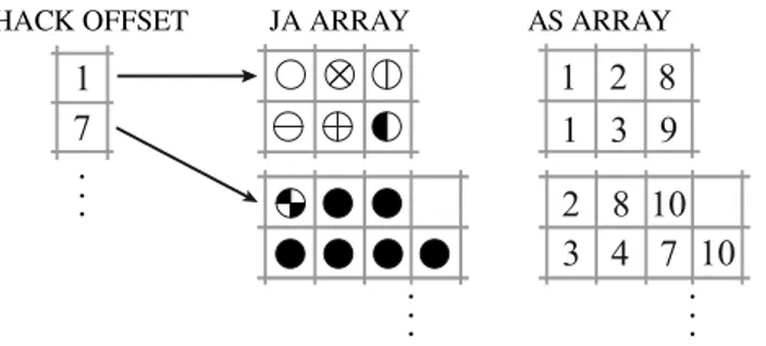
3.2 Hacked ELLPACK
The hacked ELLPACK (HLL) format alleviates the main problem of the ELLPACK format, that is, the amount of memory required by padding for sparse matrices in which the maximum row length is larger than the average. The number of elements allocated to padding is [(m ∗ maxN R) − (m ∗ avgN R) = m ∗ (maxN R − avgN R)] for both AS and JA arrays, where m is equal to the number of rows of the matrix, maxN R is the maximum number of nonzero elements in every row and avgN R is the average number of nonzeros. Therefore, a single densely populated row can seriously affect the total size of the allocation.
To limit the padding overhead, in the HLL format we break the original matrix into groups of rows (called hacks), and then store these groups as independent matrices in ELLPACK format; a very long row only affects the memory size of the hack in which it appears. The groups can be option-ally arranged selecting rows in an arbitrary order; if the rows are sorted by decreasing number of nonzeros we obtain essentially the JAgged Diagonals format, whereas if each row makes up its own group we are back to CSR storage. If the rows are not in the original order, then an additional vec-tor rIdx is required, svec-toring the actual row index for each row in the data structure.
The multiple ELLPACK-like buffers are stacked together inside a single, one dimensional array; an additional vector hackOffsets is provided to keep track of the individual submatrices. All hacks have the same number of rows hackSize; hence, the hackOffsets vector is an array of (m/hackSize) + 1 elements, each one pointing to the first index of a submatrix inside the stacked cM /rP buffers, plus an additional element pointing past the end of the last block, where the next one would begin. We thus have the property that the elements of the k-th hack are stored between hackOffsets[k] and hackOffsets[k+1], similarly to what happens in the CSR format.
HACK OFFSET JA ARRAY AS ARRAY 1 1 7 2 8 1 3 9 2 8 10 3 4 7 10
Figure 6: Hacked ELLPACK compression of matrix in Figure 1 With this data structure a very long row only affects one hack, and therefore the additional memory is limited to the hack in which the row appears. Note that if we adopt sequential ordering and choose 1 as the
group size, we have no padding and the format becomes identical to CSR; at the other extreme, if we let the group size grow to n, we have a standard ELLPACK matrix. In our CUDA implementation the hack size is chosen to be a multiple of the warp size (32), so that each submatrix has the correct alignment.
Sorting the rows of the matrix based on rows’ length (populating the above mentioned rIdx vector) may reduce the amount of padding actually needed, since large rows tend to go together in the same submatrix. However it also entails the use of permutations in computing the output vector, and therefore the overall performance may actually worsen.
The resulting data structure has proven to be very effective; over the whole set of matrices we tested, the allocation size of the resulting storage is almost the same as the size needed by the CSR format, but the sparse matrix-vector routine has a performance close to that of the ELLPACK for-mat, because coefficients and column indices are still accessed with coalesced reads by each warp. Similar to the ELL-G case, we can also use 2 or more threads per matrix row, as we will see in Section 4.
The HLL format is similar to the Sliced ELLR-T format [15], where however no provisions are made for an auxiliary ordering vector.
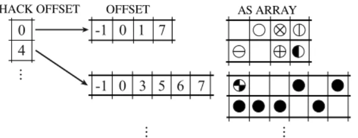
3.3 Hacked DIA
Storage by DIAgonals is an attractive option for matrices whose coefficients are located on a small set of diagonals, since they do away with storing ex-plicitly the indices and therefore reduce significantly memory traffic. How-ever, having a few coefficients outside of the main set of diagonals may significantly increase the amount of needed padding; moreover, while the DIA code is easily vectorized, it does not necessarily make optimal use of the memory hierarchy. While processing each diagonal we are updating en-tries in the output vector y, which is then accessed multiple times; if the vector y is too large to remain in the cache memory, the associated cache miss penalty is paid multiple times.
The hacked DIA (HDIA) format was designed to contain the amount of padding, by breaking the original matrix into equally sized groups of rows (hacks), and then storing these groups as independent matrices in DIA format. This approach is similar to that of HLL, and requires using an offset vector for each submatrix. Again, similarly to HLL, the various submatrices are stacked inside a linear array to improve memory management. The fact that the matrix is accessed in slices helps in reducing cache misses, especially regarding accesses to the vector y.
An additional vector hackOffsets is provided to complete the matrix for-mat; given that hackSize is the number of rows of each hack, the hackOffsets vector is made by an array of (m/hackSize) + 1 elements, pointing to the first diagonal offset of a submatrix inside the stacked offsets buffers, plus an
additional element equal to the number of nonzero diagonals in the whole matrix. We thus have the property that the number of diagonals of the k-th hack is given by hackOffsets[k+1] - hackOffsets[k].
0 0 0 4 1 7 -1 3 5 6 7 -1
HACK OFFSET OFFSET AS ARRAY
Figure 7: Hacked DIA compression of matrix in Figure 1
In our CUDA implementation the hack size is chosen to be a multiple of the warp size (32), so that each submatrix has the correct alignment.
4
Experimental results
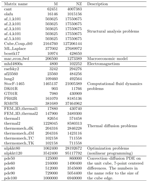
To evaluate the storage formats we have chosen a set of test matrices; some of them were taken from the Sparse Matrix Collection at the Uni-versity of Florida (UFL) [13], while some were generated from a model three-dimensional convection-diffusion PDE. Table 2 summarizes the ma-trices characteristics.
For each matrix, we report the matrix size (M rows) and the number of nonzero elements (NZ). The sparse matrices we selected from the UFL collection represent different kinds of real applications including structural analysis problems, economics, electromagnetism, computational fluid dy-namics problems, thermal diffusion problems, and optimization problems. The UFL collection has been previously used in other works regarding SpMV on GPUs, among them [3, 7, 17, 18, 28, 30]. The UFL collection subset we selected includes some large sparse matrices (namely, Cube Coup dt0, StocF-1465, nlpkkt80, and nlpkkt120) i.e., matrices having more than 1 million rows and 12 million nonzero coefficients. Since the irregular access pattern to the GPU memory can significantly affect performance of GPU implementations when evaluating larger matrices [10], it is important to in-clude large sparse matrices in the performance evaluation. This is in our opinion a limitation of some previously published works on the subject.
The model PDE sparse matrices arise from a three-dimensional convection-diffusion PDE discretized with centered finite differences on the unit cube. This scheme gives rise to a matrix with at most 7 nonzero elements per row: the matrix size is expressed in terms of the length of the cube edge, so that the case pde10 corresponds to a 1000 × 1000 matrix. We already used this collection in [5].
Table 2: Sparse matrices used in the experiments and their attributes
Matrix name M NZ Description
cant 62451 4007383
Structural analysis problems olafu 16146 1015156 af 1 k101 503625 17550675 af 2 k101 503625 17550675 af 3 k101 503625 17550675 af 4 k101 503625 17550675 af 5 k101 503625 17550675 Cube Coup dt0 2164760 127206144 ML Laplace 377002 27689972 bcsstk17 10974 428650
mac econ fwd 206500 1273389 Macroeconomic model mhd4800a 4800 102252 Electromagnetism raefsky2 3242 294276
Computational fluid dynamics problems af23560 23560 484256 lung2 109460 492564 StocF-1465 1465137 21005389 DK01R 903 11766 GT01R 7980 430909 PR02R 161070 8185136 RM07R 381689 37464962 FEM 3D thermal1 17880 430740
Thermal diffusion problems FEM 3D thermal2 147900 3489300 thermal1 82654 574458 thermal2 1228045 8580313 thermomech dK 204316 2846228 thermomech dM 204316 1423116 thermomech TC 102158 711558 thermomech TK 102158 711558 nlpkkt80 1062400 28192672 Optimization problems (nonlinear programming) nlpkkt120 3542400 95117792
pde50 125000 860000 Convection–diffusion PDE on the unit cube, 7-point centered differences. The numbers in the name refer to the size of the cube edge.
pde60 216000 1490400 pde80 512000 3545600 pde90 729000 5054400 pde100 1000000 6940000
The performance measurements were taken on three different platforms, whose characteristics are reported in Table 3. Table 4 summarizes the spec-ifications of the GPUs on such platforms. The experiments were run using the GCC compiler suite and the CUDA programming toolkit; on platform 1 we used GCC 4.9 (development) and CUDA 5.5, on platform 2 GCC 4.7.2 and CUDA 4.2.9, on platform 3 GCC 4.6.3 and CUDA 6.0.
For all matrices we tested all the formats we have proposed, and we compare them to the Hybrid format available in the NVIDIA cuSPARSE library. The hybrid format is documented by NVIDIA to be a mixture of
Table 3: Test platforms characteristics
Platform CPU GPU
1 AMD Athlon 7750 GTX 285 2 Xeon E5645 M2070 3 AMD FX 8120 GTX 660
Table 4: GPU model specifications
GTX 285 M2070 GTX 660 Multiprocessors 30 14 5
Cores 240 448 960
Clock 1548 MHz 1150 MHz 1033 MHz DP peak 92.9 GFlop/s 515.2 GFlop/s 82.6 GFlop/s Bandwidth 162.4 GB/s 150.3 GB/s 144.2 GB/s Compute capability 1.3 2.0 (Fermi) 3.0 (Kepler)
ELLPACK and coordinate, attempting to overcome the memory overhead of the full ELLPACK. The CuSPARSE library allows the user to control the partition of the input matrix into an ELLPACK part and a coordinate part; for the purposes of our comparison we always used the library default choice.
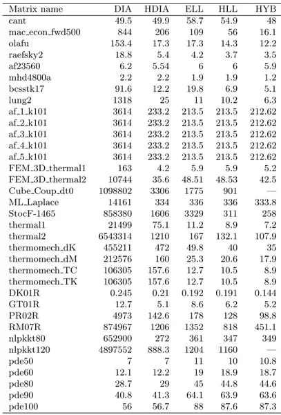
Considering the amount of memory employed by the various storage for-mats, we see that in many cases HLL and HYB achieve a similar occupancy, with the advantage going either way. For some matrices the ELLPACK storage format is essentially equivalent to HLL, meaning that the maximum and average row lengths are very close; this is true for instance of the AF matrices. The PDE model matrices also have a very regular structure and similar occupancy between ELL, HLL and HYB; however they also have a native diagonal structure that makes them natural candidates for the DIA and HDIA formats. From Table 5 this is also true of FEM 3D thermal2 (at least for the HDIA), and of DK01R/GT01R/PRO2R/RM07R; many other matrices do not have a natural diagonal structure and the resulting fill-in destroys any performance advantage to be gained.
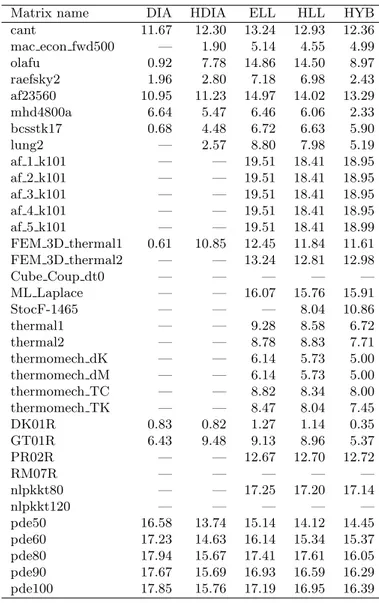
On platform 1 (GTX 285), we see from Table 6 that the HLL and HYB formats are essentially equivalent in performance. On platform 2 (M 2050) this is still largely true except for the model PDE problem at large sizes, but even there the difference is quite small; on platform 3 (GTX 660) the difference for the model PDE problems is again very small.
For the model PDE matrices, FEM 3D thermal2 and the nlpkktXX on platforms 2 and 3 the HDIA format is substantially better than either HLL
or HYB; it is not quite clear why this does not happen on the older card of platform 1. It is apparent that a diagonal-based format should not be used unless there is a natural diagonal structure to the matrix, but this structure may not be immediately visible. Indeed for the nlp matrices the HDIA format performs very well, even though the DIA format is unmanageable.
One further set of tests was run to compare our results with ELLR-T [39] and to assess the viability of using multiple threads per row. On platform 1 we could not run the tests with ELLR-T because the library distributed by the authors from their web site would not run properly on the GTX 285, and sources were not available for recompilation. Therefore in Table 9 we report performance at 1 and 2 threads for both ELL-G and HLL-G formats. We see that it is very rarely the case that the 2-threads version gains any advantage, and even when it does, it is only a very slight one. Similar results on platform 2 are shown in Table 10.
On platform 3 we compare our ELL-G code run with 1 and 2 threads with the ELLR-T code run with 1, 2 and 4 threads. The results are different in that there are even less cases where multiple threads are favourable, e.g., the af 1 k101 through af 5 k101 matrices show a degradation as opposed to the slight improvement they had on platform 1. In all cases the performance of our code is on par or slightly faster than that of the ELLR-T code.
In conclusion we wish to notice that finding the best match between storage format, matrix structure and computing device is an entirely nonob-vious proposition, even when confining ourselves to similar devices such as the NVIDIA GPUs. This means that the flexibility of the PSBLAS object framework outlined in [19, 5] is instrumental to extract the best performance in a convenient way, especially when dealing with heterogeneous computing platforms.
5
Conclusions
In this paper we dealt with the sparse matrix-vector multiplication and its implementation on GPGPUs. We presented three novel matrix formats: ELL-G and HLL which both derive from ELL, and HDIA for matrices hav-ing mostly a diagonal sparsity pattern. We have explored the performance attainable accounting for variations in the matrix structure, the storage for-mat and the computing device, and we have shown how it is desirable to have a flexible framework that enables to switch among various formats at the user’s choice.
We have so far limited ourselves to storage formats that can be seen, at least to some extent, as general purpose; in particular, we plan to consider in future work matrices that have block-entry structures, since those matrices do not appear in all applications.
it/psblas.
Acknowledgements
We gratefully acknowledge the support we have received from CINECA for project IsC14 HyPSBLAS, under the ISCRA grant programme for 2014, and from Amazon with the AWS in Education Grant programme 2014.
Table 5: Memory occupancy in MB
Matrix name DIA HDIA ELL HLL HYB
cant 49.5 49.9 58.7 54.9 48 mac econ fwd500 844 206 109 56 16.1 olafu 153.4 17.3 17.3 14.3 12.2 raefsky2 18.8 5.4 4.2 3.7 3.5 af23560 6.2 5.54 6 6 5.9 mhd4800a 2.2 2.2 1.9 1.9 1.2 bcsstk17 91.6 12.2 19.8 6.9 5.1 lung2 1318 25 11 10.2 6.3 af 1 k101 3614 233.2 213.5 213.5 212.62 af 2 k101 3614 233.2 213.5 213.5 212.62 af 3 k101 3614 233.2 213.5 213.5 212.62 af 4 k101 3614 233.2 213.5 213.5 212.62 af 5 k101 3614 233.2 213.5 213.5 212.62 FEM 3D thermal1 163 4.2 5.9 5.9 5.2 FEM 3D thermal2 10744 35.6 48.51 48.53 42.5 Cube Coup dt0 1098802 3306 1775 901 — ML Laplace 14161 334 336 336 333.8 StocF-1465 858380 1606 3329 311 258 thermal1 21499 75.1 11.2 8.9 7.2 thermal2 6543314 1210 167 132.1 107.9 thermomech dK 455211 472 49.8 40 35 thermomech dM 212576 160 25.3 20.6 17.9 thermomech TC 106305 157.6 12.7 10.5 8.9 thermomech TK 106305 157.6 12.7 10.5 8.9 DK01R 0.245 0.21 0.192 0.191 0.144 GT01R 12.7 5.1 8.6 6.2 5.2 PR02R 4973 142.6 178 128 98.8 RM07R 874967 1206 1352 818 451.1 nlpkkt80 652900 272 361 347 349 nlpkkt120 4897552 888.3 1204 1160 — pde50 7 7 11 10 10.8 pde60 12.1 12.2 19 18.9 18.7 pde80 28.7 29 45 44.8 44.6 pde90 40.8 41.3 64.1 63.9 63.6 pde100 56 56.7 88 87.6 87.3
Table 6: Performance on platform 1 (GFLOPS)
Matrix name DIA HDIA ELL HLL HYB cant 11.67 12.30 13.24 12.93 12.36 mac econ fwd500 — 1.90 5.14 4.55 4.99 olafu 0.92 7.78 14.86 14.50 8.97 raefsky2 1.96 2.80 7.18 6.98 2.43 af23560 10.95 11.23 14.97 14.02 13.29 mhd4800a 6.64 5.47 6.46 6.06 2.33 bcsstk17 0.68 4.48 6.72 6.63 5.90 lung2 — 2.57 8.80 7.98 5.19 af 1 k101 — — 19.51 18.41 18.95 af 2 k101 — — 19.51 18.41 18.95 af 3 k101 — — 19.51 18.41 18.95 af 4 k101 — — 19.51 18.41 18.95 af 5 k101 — — 19.51 18.41 18.99 FEM 3D thermal1 0.61 10.85 12.45 11.84 11.61 FEM 3D thermal2 — — 13.24 12.81 12.98 Cube Coup dt0 — — — — — ML Laplace — — 16.07 15.76 15.91 StocF-1465 — — — 8.04 10.86 thermal1 — — 9.28 8.58 6.72 thermal2 — — 8.78 8.83 7.71 thermomech dK — — 6.14 5.73 5.00 thermomech dM — — 6.14 5.73 5.00 thermomech TC — — 8.82 8.34 8.00 thermomech TK — — 8.47 8.04 7.45 DK01R 0.83 0.82 1.27 1.14 0.35 GT01R 6.43 9.48 9.13 8.96 5.37 PR02R — — 12.67 12.70 12.72 RM07R — — — — — nlpkkt80 — — 17.25 17.20 17.14 nlpkkt120 — — — — — pde50 16.58 13.74 15.14 14.12 14.45 pde60 17.23 14.63 16.14 15.34 15.37 pde80 17.94 15.67 17.41 17.61 16.05 pde90 17.67 15.69 16.93 16.59 16.29 pde100 17.85 15.76 17.19 16.95 16.39
Table 7: Performance on platform 2 (GFLOPS)
Matrix DIA HDIA ELL HLL HYB cant 13.63 13.04 11.83 11.59 12.35 mac econ fwd500 0.27 1.03 3.53 3.53 4.74 olafu 1.17 7.40 11.04 10.49 10.65 raefsky2 2.00 2.92 10.21 10.06 4.89 af23560 11.84 10.73 12.28 12.20 11.94 mhd4800a 5.30 5.11 6.42 5.81 3.65 bcsstk17 0.80 4.12 7.29 7.16 7.57 lung2 0.09 3.03 6.58 6.54 5.50 af 1 k101 0.90 12.44 14.15 14.14 15.16 af 2 k101 0.90 12.44 14.15 14.14 15.16 af 3 k101 0.90 12.44 14.15 14.14 15.16 af 4 k101 0.90 12.44 14.15 14.14 15.16 af 5 k101 0.90 12.45 14.15 14.14 15.16 FEM 3D thermal1 0.61 12.82 11.37 14.14 13.49 FEM 3D thermal2 — 15.25 11.56 10.75 13.07 Cube Coup dt0 — 6.60 10.56 10.69 — ML Laplace — 14.21 14.31 14.24 14.83 StocF-1465 — 2.26 9.40 9.19 10.66 thermal1 — 1.30 8.17 7.95 6.90 thermal2 — 1.26 7.74 7.64 7.00 thermomech dK — 0.87 7.88 7.78 7.75 thermomech dM — 1.31 5.77 5.70 6.08 thermomech TC — 0.77 5.38 5.35 5.09 thermomech TK — 0.77 5.38 5.35 5.09 DK01R 0.61 0.61 2.58 2.47 0.68 GT01R 7.74 9.91 10.11 9.99 7.70 PR02R — 9.63 10.48 10.43 10.50 RM07R — 5.18 8.34 8.44 9.08 nlpkkt80 — 15.62 13.14 13.10 15.05 nlpkkt120 — 15.00 12.97 12.94 14.01 pde50 15.84 14.79 11.83 11.96 12.43 pde60 16.37 15.43 12.02 12.17 12.93 pde80 16.76 16.02 12.05 12.37 13.30 pde90 16.58 16.04 11.94 12.27 13.16 pde100 16.29 15.95 11.78 12.18 13.37
Table 8: Performance on platform 3 (GFLOPS)
Matrix name DIA HDIA ELL HLL HYB cant 17.1 16.9 15.34 14.73 14.7 mac econ fwd500 0.3 1.3 4.9 4.42 5.6 olafu 1.6 11.3 14.9 13.9 11.96 raefsky2 2.7 4.6 12.6 12.3 4.5 af23560 13.5 15.2 15.2 14.47 14.4 mhd4800a 5.8 5.8 8.0 7 3.7 bcsstk17 0.9 6.4 9.45 8.19 7.0 lung2 0.1 3.8 8.0 7.46 5.1 af 1 k101 — 15.9 18.3 18.1 17.8 af 2 k101 — 15.9 18.3 18.1 17.8 af 3 k101 — 15.9 18.3 18.1 17.8 af 4 k101 — 15.9 18.3 18.1 17.8 af 5 k101 — 15.9 18.3 18.1 17.8 FEM 3D thermal1 0.7 15.62 14.0 13.65 14.8 FEM 3D thermal2 — 19.3 14.6 14.34 15.4 Cube Coup dt0 — — — 10.7 — ML Laplace — 18.7 18.3 18.44 18.0 StocF-1465 — 2.2 — 12.32 13.7 thermal1 — 1.7 10.2 9.9 8.5 thermal2 — 1.6 9.27 9.54 8.3 thermomech dK — 1.1 9.0 10.17 8.4 thermomech dM — 1.56 6.2 6.6 6.5 thermomech TC — 0.92 6.36 6.39 6.5 thermomech TK — 0.92 6.36 6.39 6.5 DK01R 0.7 0.644 2.1 2.07 0.58 GT01R 9 13.1 12.0 12.64 8.7 PR02R — 12.8 13.4 13.74 13.6 RM07R — 6.9 6.5 12.3 11.0 nlpkkt80 — 21.28 16.7 16.8 16.7 nlpkkt120 — 21.5 16.6 16.7 — pde50 17.6 17.4 15.0 14.5 14.3 pde60 19.5 18.6 15.5 15 14.7 pde80 19.3 18.43 15.0 14.7 14.9 pde90 18.3 17.6 14.4 14 14.6 pde100 17.4 17.16 13.7 13.7 13.3
Table 9: Performance on platform 1, multiple threads (GFLOPS) Matrix ELL-G HLL-G threads threads 1 2 1 2 cant 13.24 14.57 12.93 13.92 mac econ fwd500 5.14 4.74 4.55 5.15 olafu 14.86 14.29 14.50 13.18 raefsky2 7.18 11.73 6.98 9.82 af23560 14.97 14.81 14.02 12.10 mhd4800a 6.46 8.07 6.06 6.79 bcsstk17 6.72 9.64 6.63 8.69 lung2 8.80 8.53 7.98 6.80 af 1 k101 19.51 20.38 18.41 20.22 af 2 k101 19.51 20.48 18.41 20.22 af 3 k101 19.51 20.48 18.41 20.22 af 4 k101 19.51 20.49 18.41 20.22 af 5 k101 19.51 20.49 18.41 20.22 FEM 3D thermal1 12.45 11.76 11.84 10.35 FEM 3D thermal2 13.24 13.78 12.81 13.55 ML Laplace 16.07 17.54 15.76 17.50 StocF-1465 0.00 0.00 8.04 9.06 thermal1 9.28 8.74 8.58 7.45 thermal2 8.78 8.56 8.83 8.10 thermomech dK 6.14 6.05 5.73 5.62 thermomech dM 6.14 6.04 5.73 5.62 thermomech TC 8.82 10.26 8.34 9.37 thermomech TK 8.47 8.26 8.04 7.40 DK01R 1.27 1.64 1.14 1.30 GT01R 9.13 10.89 8.96 9.93 PR02R 12.67 14.60 12.70 14.40 nlpkkt80 17.25 18.03 17.20 18.45 pde50 15.14 14.34 14.12 11.40 pde60 16.14 14.80 15.34 11.83 pde80 17.41 15.27 17.61 12.50 pde90 16.93 15.03 16.59 12.63 pde100 17.19 15.30 16.95 12.72
Table 10: Performance on platform 2, multiple threads (GFLOPS) Matrix ELL-G HLL-G threads threads 1 2 1 2 cant 11.83 11.91 11.59 11.92 mac econ fwd500 3.53 3.71 3.53 3.69 olafu 11.04 11.34 10.49 11.25 raefsky2 10.21 12.27 10.06 11.82 af23560 12.28 11.78 12.20 11.36 mhd4800a 6.42 6.20 5.81 5.83 bcsstk17 7.29 8.24 7.16 8.19 lung2 6.58 5.77 6.54 5.52 af 1 k101 14.15 14.34 14.14 14.35 af 2 k101 14.15 14.31 14.14 14.35 af 3 k101 14.15 14.33 14.14 14.35 af 4 k101 14.15 14.32 14.14 14.35 af 5 k101 14.15 14.33 14.14 14.35 FEM 3D thermal1 11.37 10.83 10.75 10.47 FEM 3D thermal2 11.56 11.65 11.32 11.77 ML Laplace 14.31 14.57 14.24 14.70 StocF-1465 9.40 9.19 9.32 9.03 thermal1 8.17 6.96 7.95 6.73 thermal2 7.74 6.86 7.64 6.78 thermomech dK 7.88 7.29 7.78 7.23 thermomech dM 5.77 5.42 5.70 5.49 thermomech TC 5.38 5.16 5.35 5.20 thermomech TK 5.38 5.16 5.35 5.20 DK01R 2.58 2.58 2.47 2.46 GT01R 10.11 9.47 9.99 9.32 PR02R 10.48 10.09 10.43 10.16 RM07R 8.34 8.31 8.44 8.41 nlpkkt80 13.14 13.27 13.10 13.21 nlpkkt120 12.97 13.21 12.94 13.32 pde50 11.83 8.94 11.96 8.58 pde60 12.02 9.03 12.17 8.72 pde80 12.05 8.96 12.37 8.73 pde90 11.94 8.54 12.27 8.41 pde100 11.78 8.35 12.18 8.21
Table 11: Performance on platform 3, multiple threads (GFLOPS)
Matrix ELL-G HLL-G ELLRT
threads threads threads
1 2 1 2 1 2 4 cant 15.34 16.14 14.73 16.32 15 16.2 16.4 mac econ fwd500 4.9 2 4.61 4.44 5 4.5 4.42 4.65 olafu 14.9 14.37 13.9 14.7 14.2 14.4 14.5 raefsky2 12.64 15.63 12.3 15.9 9.85 15.12 14.38 af23560 15.23 15.29 14.47 14.87 14.77 14.31 12.56 mhd4800a 8 8.17 7 7.76 7.48 6.7 7.9 bcsstk17 9.45 10.6 8.19 11 8.5 10.5 11.2 lung2 7.97 7.8 7.46 7 7.5 6.32 5.95 af 1 k101 18.3 18.8 18.1 18.84 18.3 17.6 16.8 af 2 k101 18.3 18.8 18.1 18.84 18.3 17.6 16.8 af 3 k101 18.3 18.8 18.1 18.84 18.3 17.6 16.8 af 4 k101 18.3 18.8 18.1 18.84 18.3 17.6 16.8 af 5 k101 18.3 18.8 18.1 18.84 18.3 17.6 16.8 FEM 3D thermal1 14 13.7 13.65 13.36 14.33 13.7 12.63 FEM 3D thermal2 14.6 15.23 14.34 15.2 14.76 14.72 13.8 Cube Coup dt0 — — 10.7 11.2 10.7 11.51 11.7 ML Laplace 18.3 19 18.44 19.2 18.6 18.78 17.87 StocF-1465 - - 12.32 12.50 - - -thermal1 10.2 8.4 9.9 8.6 10 7.6 7.4 thermal2 9.27 7.8 9.54 7.87 9.27 7.2 7.5 thermomech dK 8.96 8.76 10.17 9.8 8.7 9.16 7.6 thermomech dM 6.25 5.8 6.6 6.3 6.25 6 6.2 thermomech TC 6.36 6.5 6.39 6.8 6.7 5.7 6.5 thermomech TK 6.36 6.5 6.39 6.8 6.7 5.7 6.5 DK01R 2.1 2.07 2.07 2.07 2.36 2.39 2.34 GT01R 12.66 12 12.64 12 12 10.47 11.63 PR02R 13.45 13.71 13.74 13.72 13.86 13.63 13.16 RM07R 6.46 12 12.3 12.25 6.66 6.78 8.2 nlpkkt80 16.65 17.4 16.78 16.9 16.47 15.1 12.17 nlpkkt120 16.63 16.1 16.66 15.59 17 16.6 15.22 pde50 15 11.73 14.5 11 14.53 9.6 8.98 pde60 15.5 11.78 15 10.7 15.02 9.6 8.85 pde80 15 11.58 14.7 10.14 15.18 9.1 8.81 pde90 14.4 11.24 14 10.3 14.78 9.5 8.82 pde100 13.7 11.2 13.7 10.45 13.7 9.8 8.8
References
[1] E. Anderson, Z. Bai, C. Bischof, S. Blackford, J. Demmel, J. Don-garra, J. Du Croz, A. Greenbaum, S. Hammarling, A. McKenney, and D. Sorensen. LAPACK Users’ Guide. SIAM, 3rd edition, 1999.
[2] D. Barbieri, V. Cardellini, and S. Filippone. Generalized GEMM appli-cations on GPGPUs: experiments and appliappli-cations. In Parallel Com-puting: from Multicores and GPU’s to Petascale, ParCo ’09, pages 307– 314. IOS Press, 2010.
[3] M. M. Baskaran and R. Bordawekar. Optimizing sparse matrix-vector multiplication on GPUs. Technical Report RC24704, IBM Research, 2009.
[4] N. Bell and M. Garland. Implementing sparse matrix-vector multipli-cation on throughput-oriented processors. In Proc. of Int’l Conf. on High Performance Computing Networking, Storage and Analysis, SC ’09, pages 18:1–18:11. ACM, 2009.
[5] V. Cardellini, S. Filippone, and Damian Rouson. Design patterns for sparse-matrix computations on hybrid CPU/GPU platforms. Sci. Pro-gram., 22(1):1–19, 2014.
[6] J. Choi, J. Demmel, J. Dhillon, J. Dongarra, S. Ostrouchov, A. Petitet, K. Stanley, D. Walker, and R. C. Whaley. ScaLAPACK: A portable linear algebra library for distributed memory computers. LAPACK Working Note #95, University of Tennessee, 1995.
[7] J. W. Choi, A. Singh, and R. W. Vuduc. Model-driven autotuning of sparse matrix-vector multiply on GPUs. SIGPLAN Not., 45:115–126, January 2010.
[8] P Colella. Defining Software Requirements for Scientific Comput-ing, 2004. http://view.eecs.berkeley.edu/w/images/temp/6/6e/ 20061003235551!DARPAHPCS.ppt.
[9] CUSP : A C++ Templated Sparse Matrix Library, 2015. http:// cusplibrary.github.io.
[10] H.-V. Dang and B. Schmidt. CUDA-enabled sparse matrix-vector multiplication on GPUs using atomic operations. Parallel Comput., 39(11):737–750, 2013.
[11] T. Davis. Wilkinson’s sparse matrix definition. NA Digest, 07(12):379– 401, March 2007.
[12] T. A. Davis. Algorithm 832: UMFPACK V4.3—an unsymmetric-pattern multifrontal method. ACM Trans. Math. Softw., 30(2):196–199, 2004.
[13] T. A. Davis and Y. Hu. The University of Florida Sparse Matrix Col-lection. ACM Trans. Math. Softw., 38(1):1:1–1:25, 2011.
[14] I.S. Duff, M. Marrone, G. Radicati, and C. Vittoli. Level 3 basic linear algebra subprograms for sparse matrices: a user level interface. ACM Trans. Math. Softw., 23(3):379–401, 1997.
[15] A. Dziekonski, A. Lamecki, and M. Mrozowski. A memory efficient and fast sparse matrix vector product on a GPU. Progress in Electromag-netics Research, 116:49–63, 2011.
[16] EESI Working Group 4.3. Working group report on numerical libraries, solvers and algorithms. Technical report, European Exascale Software Initiative, December 2011. Available from http://www.eesi-project. eu/.
[17] X. Feng, H. Jin, R. Zheng, K. Hu, J. Zeng, and Z. Shao. Optimization of sparse matrix-vector multiplication with variant CSR on GPUs. In Proc. of 17th Int’l Conf. on Parallel and Distributed Systems, ICPADS ’11, pages 165–172. IEEE Computer Society, 2011.
[18] X. Feng, H. Jin, R. Zheng, Z. Shao, and L. Zhu. A segment-based sparse matrix vector multiplication on CUDA. Concurr. Comput.: Pract. Ex-per., 26(1):271–286, 2014.
[19] S. Filippone and A. Buttari. Object-oriented techniques for sparse matrix computations in Fortran 2003. ACM Trans. Math. Softw., 38(4):23:1–23:20, 2012.
[20] A. Greenbaum. Iterative Methods for Solving Linear Systems. SIAM, Philadelphia, PA, 1997.
[21] M. R. Hestenes and E. Stiefel. Methods of conjugate gradients for solving linear systems. J. Res. Natl. Bur. Stand., 49:409–436, 1952. [22] W. W. Hwu. GPU Computing Gems Emerald Edition. Morgan
Kauf-mann Publishers Inc., San Francisco, CA, 2011.
[23] C. T. Kelley. Iterative Methods for Linear and Nonlinear Equations. SIAM, Philadelphia, 1995.
[24] D. R Kincaid, T. C. Oppe, and D. M. Young. ITPACKV 2D User’s Guide, May 1989. http://rene.ma.utexas.edu/CNA/ITPACK/ manuals/userv2d/.
[25] M. Kreutzer, G. Hager, G. Wellein, H. Fehske, A. Basermann, and A. R. Bishop. Sparse matrix-vector multiplication on GPGPU clusters: A new storage format and a scalable implementation. In Proc. of 26th IEEE Int’l Parallel and Distributed Processing Symposium Workshops & PhD Forum, IPDPSW ’12, pages 1696–1702, 2012.
[26] Randall J. LeVeque. Finite Difference Methods for Ordinary and Partial Differential Equations. SIAM, Philadelphia, PA, 2007.
[27] David Luebke, Mark Harris, Naga Govindaraju, Aaron Lefohn, Mike Houston, John Owens, Mark Segal, Matthew Papakipos, and Ian Buck. GPGPU: general-purpose computation on graphics hardware. In Proc. of 2006 ACM/IEEE Conf. on Supercomputing, SC ’06, 2006.
[28] K.K. Matam and K. Kothapalli. Accelerating sparse matrix vector multiplication in iterative methods using GPU. In Proc. of 40th Int’l Conf. on Parallel Processing, ICPP ’11, pages 612–621. IEEE Computer Society, September 2011.
[29] A. Monakov, A. Lokhmotov, and A. Avetisyan. Automatically tuning sparse matrix-vector multiplication for GPU architectures. In High Performance Embedded Architectures and Compilers, volume 5952 of LNCS, pages 111–125. Springer-Verlag, 2010.
[30] D. Mukunoki and D. Takahashi. Optimization of sparse matrix-vector multiplication for CRS format on NVIDIA Kepler architecture GPUs. In Computational Science and Its Applications, volume 7975 of LNCS, pages 211–223. Springer, 2013.
[31] J. Nickolls, I. Buck, M. Garland, and K. Skadron. Scalable parallel programming with CUDA. ACM Queue, 6:40–53, March 2008.
[32] NVIDIA Corp. CUDA cuSPARSE library, 2015. http://developer. nvidia.com/cusparse.
[33] S. V. Patankar. Numerical Heat Transfer and Fluid Flow. Series in Computational Methods in Mechanics and Thermal Sciences. Hemi-sphere Publishing Corp., NY, first edition, 1980.
[34] J. C. Pichel, F. F. Rivera, M. Fern´andez, and A. Rodr´ıguez. Optimiza-tion of sparse matrix-vector multiplicaOptimiza-tion using reordering techniques on GPUs. Microprocess. Microsyst., 36(2):65–77, 2012.
[35] A. Quarteroni and A. Valli. Numerical Approximation of Partial Dif-ferential Equations. Springer-Verlag, Berlin, 1994.
[36] Y. Saad. Iterative Methods for Sparse Linear Systems. Society for Industrial and Applied Mathematics, Philadelphia, PA, 2nd edition, 2003.
[37] J. Sanders and E. Kandrot. CUDA by example: An introduction to general-purpose GPU programming. Addison-Wesley, Boston, MA, USA, first edition, 2010.
[38] F. V´azquez, J. J. Fern´andez, and E. M. Garz´on. A new approach for sparse matrix vector product on NVIDIA GPUs. Concurr. Comput.: Pract. Exper., 23(8):815–826, 2011.
[39] F. V´azquez, J.J. Fern´andez, and E. M. Garz´on. Automatic tuning of the sparse matrix vector product on GPUs based on the ELLR-T approach. Parallel Comput., 38(8):408–420, 2012.
[40] V. Volkov and J. W. Demmel. Benchmarking GPUs to tune dense linear algebra. In Proc. of 2008 ACM/IEEE Conf. on Supercomputing, SC ’08, pages 31:1–31:11, 2008.
[41] S. Williams, A. Waterman, and D. Patterson. Roofline: An insightful visual performance model for multicore architectures. Commun. ACM, 52(4):65–76, April 2009.