Large deviations for risk processes with reinsurance

Large deviations for risk processes with reinsurance

Abstract

We consider risk processes with reinsurance. A general family of reinsurance contracts is allowed, including proportional and excess-of-loss policies. The claim occurrence is regulated by a classical compound Poisson process or by a Markov modulated compound Poisson process. We provide some large deviation results concerning these two risk processes in the small claim case. Finally we derive the so called Lundberg’s estimate for the ruin probabilities, and we present a numerical example.

Keywords: Large deviations, risk process, reinsurance, ruin probability, Lundberg’s estimate.

2000 Mathematics Subject Classification: 60F10, 91B30, 62P05.

1

Introduction

The model without reinsurance. We consider the risk process (Xx_{(t)) defined by}

Xx(t) = x + pt − S(t) (1)

where x > 0 is the initial capital, p > 0 is the (constant) premium rate and the aggregate claims process (S(t)) is a compound Poisson process (classical case) or a Markov modulated compound Poisson process (Markov modulated case). More precisely we have S(t) = PN (t)_k=1 Uk and N (t) =

P

k≥11Tk≤t, where (Uk) is a sequence of positive random variables and (N (t)) is a counting process

with points (T_k); further details will be given when we present the classical case and the Markov modulated case separately. Roughly speaking, when we deal with the Markov modulated case, claims intensity and claims size distribution depend on the evolution of a finite state space Markov chains; from the actuarial point of view the Markov chain describes the environmental conditions that influence the phenomena, such as weather conditions in car insurance.

We assume that the random variables (Uk) have finite expected values and that S(t)_t converges

to some limit value ` as t → ∞. The (infinite horizon) ruin probabilities (ψ(x))x>0 are defined by

ψ(x) = P (τx < ∞), where τx= inf{t ≥ 0 : Xx(t) < 0}

and, in order to avoid the trivial case ψ(x) = 1 for all x > 0, the so called net profit condition is required, i.e. p = (1 + κ)` for some relative safety loading κ > 0.

∗_{Dipartimento di Matematica, Universit`a di Roma ”Tor Vergata”, Via della Ricerca Scientifica, I-00133 Rome,}

Italy. e-mail: macci@mat.uniroma2.it

†_{Dipartimento di Matematica per le Decisioni Economiche Finanziarie ed Assicurative, Universit`a di Roma ”La}

Reinsurance policies. In our model reinsurance is allowed, i.e. the insurance company may insure part of the risk at another company (the reinsurance company) in return for a part of the premium pt. A reinsurance policy is described by a measurable function R : [0, ∞) × [0, ∞) → [0, ∞), for which we use the notation R(t, α) = Rt(α); for such a function we require the condition

0 ≤ Rt(α) ≤ α for all t, α ≥ 0. This means that Rt(α) is the part of the claim that the company

pays when a claim of size α occurs at time t. Since the reinsurance policy is chosen dynamically, the premium rate for the reinsurer is in general not constant in time, as it happen in the classical risk model. We denote with qR(t) the premium up to time t paid by the insurer to the reinsurer,

and we shall see in detail below its determination. We assume that reinsurer uses the expected value principle with relative safety loading η > 0 for premium calculation. We shall point out below that it is interesting to consider η > κ, i.e. the case in which reinsurance is more expensive than insurance, otherwise the insurer would reinsure the whole portfolio. In conclusion the reserve process (Xx

R(t)) under the reinsurance policy R is defined by

( Xx R(t) = x + pR(t) − SR(t), where SR(t) = P_{N (t)} k=1 RTk(Uk) and pR(t) = pt − qR(t). (2) Large deviations and outline of the paper. In this paper we present some large deviation results concerning the risk process under the reinsurance policy R and we refer to the claim surplus process (Z_R(t)) defined by

Z_R(t) = x − X_Rx(t) = S_R(t) − p_R(t).

In particular we refer to the concept of large deviation principle (see e.g. Dembo and Zeitouni [4], pages 4-5, for the definition); from now on we write LDP for short. We present two kinds of LDPs. The first one concerns the classical case (section 2) and it is a sample path large deviation result because it is a LDP on the space of c`adl`ag functions D[0, 1]; the second one concerns the Markov modulated case (section 3) and it is a LDP on R. More precisely (we use the standard notation B◦ _{for the interior of B and B for the closure of B) in the first case we have}

− inf f ∈B◦IR(f ) ≤ lim inf_α→∞ 1 αlog P ³ ZR(α·) α ∈ B ´ ≤ lim sup α→∞ 1 αlog P ³ ZR(α·) α ∈ B ´ ≤ − inf f ∈BIR(f )

for all Borel set B in D[0, 1], where IR is the rate function; in the second case we have

− inf

y∈B◦Λ

∗

R(y) ≤ lim inf_t→∞

1 t log P ³ Z_R(t) t ∈ B ´ ≤ lim sup t→∞ 1 t log P ³ Z_R(t) t ∈ B ´ ≤ − inf y∈B Λ∗_R(y) for all Borel set B in R, where Λ∗

R is the rate function. It is useful to point out that IR is a good

rate function, i.e. the level sets of IR

{f ∈ D[0, 1] : IR(f ) ≤ c} (for all c > 0)

are compact sets.

The Markov modulated case is a generalization of the classical case. The proof of the sample path LDP concerning the classical case is based on Proposition 2.1, which is a known result in the literature. For the Markov modulated case we do not have an analogous sample path large deviation result, so that we can only prove the LDP on R.

In section 4 we present some results for the ruin probabilities (ψ_R(x))_x>0 under the reinsurance policy R, which are defined by

ψR(x) = P (τRx < ∞), where τRx = inf{t ≥ 0 : XRx(t) < 0}. (3)

In subsection 4.1 we prove the so called Lundberg’s estimate for the ruin probabilities in (3); this estimate shows that, in a sense related to large deviations, ψ_R(x) decays exponentially as x → ∞. Some comments and a numerical example are presented in subsection 4.2.

The hypothesis (H) for the reinsurance policies. Since we have in mind two prototype examples of reinsurance policies presented below, in all the results in this paper we refer to the following condition:

(H): Let R∞ : [0, ∞) → [0, ∞) be a measurable function. Then for all ε > 0 there exists tε such

that for all t ≥ tε we have |Rt(α) − R∞(α)| ≤ ε max{α, 1} for all α ≥ 0.

One could consider the bound α + 1 which is simpler than max{α, 1} (but it is larger); in such a case some details presented in the paper have to be accordingly changed.

We remark that, when (H) holds, we have the pointwise convergence of Rt to R∞ as t → ∞:

lim

t→∞Rt(α) = R∞(α) for all α ≥ 0. (4)

Indeed for all ε > 0 and for all α ≥ 0 let tε,αbe defined by tε,α:= tε/ max{α,1}; then, for all t ≥ tε,α,

we have |Rt(α) − R∞(α)| ≤ _max{α,1}ε max{α, 1} = ε.

Prototype example 1: proportional policies. Set Rt(α) = btα for some bt ∈ [0, 1] and assume

that limt→∞bt = b∞ ∈ [0, 1]. We check (H) as follows. Set R∞(α) = b∞α. For all ε > 0 there

exists t_ε such that |b_t− b_∞| ≤ ε for all t ≥ t_ε; thus for all t ≥ t_ε

|Rt(α) − R∞(α)| = |bt− b∞|α ≤ εα ≤ ε max{α, 1} for all α ≥ 0.

Prototype example 2: excess-of-loss policies. Set R_t(α) = min{a_t, α} for some a_t ∈ [0, ∞) and

assume that limt→∞at = a∞ ∈ [0, ∞). We check (H) as follows. Set R∞(α) = min{a∞, α}. For

all ε > 0 there exists tε such that |at− a∞| ≤ ε for all t ≥ tε; thus for all t ≥ tε

|R_t(α) − R_∞(α)| = | min{a_t, α} − min{a_∞, α}| ≤ |a_t− a_∞| ≤ ε ≤ ε max{α, 1} for all α ≥ 0.

2

Classical case

In this section we consider the model (1) where (S(t)) is a compound Poisson process. Thus we have S(t) =PN (t)_k=1 U_k and N (t) = P_k≥11_Tk≤t, where: (U_k) and (N (t)) are independent; (U_k) are i.i.d.; (N (t)) is a Poisson process with intensity λ, i.e. the random variables (Tk− Tk−1) are i.i.d.

exponentially distributed with expected value _λ1.

We assume the following superexponential condition for the random variables (U_k): (S1): E[eθU1_{] < ∞ for all θ ∈ R.}

As a consequence of (S1) the (common) expected value µ of the random variables (Uk) is finite

and S(t)_t converges to ` = λµ as t → ∞. The reserve process (X_Rx(t)) under the reinsurance policy R is defined by (2) where p_R(t) = pt − q_R(t) = (1 + κ)λµt − (1 + η)λ Z _t 0 h E[U₁] | {z } =µ −E[R_s(U₁)] i ds;

with some easy computations we have

pR(t) = (1 + η)λ

Z _t

0

E[Rs(U1)]ds − (η − κ)λµt.

In all our results we assume that (H) holds; thus we have (4), whence we obtain lim t→∞ 1 t Z _t 0 E[Rs(U1)]ds = E[R∞(U1)]; (5)

then

lim

t→∞

p_R(t)

t = pR, where pR = (1 + η)λE[R∞(U1)] − (η − κ)λµ.

The net profit condition for the insurance company under the reinsurance policy R is p_R > λE[R∞(U1)], i.e.

(1 + η)λE[R∞(U1)] − (η − κ)λµ > λE[R∞(U1)];

thus, after some easy computations, we obtain E[R∞(U1)] ≥ h 1 −κ η i µ. (6)

We point out that (6) always holds when κ ≥ η. We also need to consider the process (ZR(t))

defined by

Z_R(t) =

N (t)_X k=1

R_∞(U_k) − p_Rt.

We remark that the process (ZR(t)) and the net profit condition presented above are a

general-ization of the analogous items presented by Hald and Schmidli [6] (section 2) for the proportional reinsurance policies; for instance the process (Xb

t) in eq. (3) in [6] is the analogous of (ZR(t)). The

net profit is the same if we have (ZR(t)) in place of (ZR(t)). Finally we consider the rate function

I_R defined by I_R(f ) = ½ R₁ 0 Λ∗R( ˙f (t))dt if f ∈ AC0[0, 1] ∞ otherwise , (7) where Λ∗_R(y) = sup θ∈R

[θy − Λ_R(θ)] and Λ_R(θ) = λ(E[eθR∞(U1)_{] − 1) − p}

Rθ. (8)

Our aim is to prove Proposition 2.3, i.e. the LDP of (ZR(α·)

α ) with rate function IR as in (7). In

order to do that we shall show that (ZR(α·)

α ) is exponentially equivalent to ( ZR(α·)

α ) as α → ∞ (see

Definition 4.2.10 in [4]); then Proposition 2.3 will be proved by considering Theorem 4.2.13 in [4] and the next known result of Borovkov [2] (see also de Acosta [3] and the references cited therein). Proposition 2.1 Assume E[eθR∞(U1)_{] < ∞ for all θ ∈ R, and (H). Then (}ZR(α·)

α ) satisfies the

LDP with rate function IR as in (7). Moreover the rate function IR is good.

Some preliminaries are needed for proving Proposition 2.3. We shall use the symbol [·] to denote the integer part of a real number. Let (An) be the sequence defined by

A_n= n X k=1 ¯ ¯ ¯RTk(Uk) − R∞(Uk) ¯ ¯ ¯ and let us consider the following lemma.

Lemma 2.2 Assume (S1) and (H). Then lim_n→∞ 1

nlog E[eθAn] = 0 for all θ > 0.

Proof. Let θ > 0 be arbitrarily fixed. We have E[eθAn_{] ≥ 1 for all n ≥ 1 since θ > 0 and the}

random variable Anis nonnegative; thus we can immediately say that lim infn→∞_n1log E[eθAn] ≥ 0.

Thus we complete the proof showing that lim sup_n→∞ 1

nlog E[eθAn] ≤ 0.

The following asymptotic estimate (10) is needed. Let n ≥ 1 and ρ, r, ε > 0 be arbitrarily fixed. Then we have

and therefore lim sup_n→∞ 1

nlog P (N (r)) ≥ [nε]) ≤ −ρε; thus, since ρ > 0 is arbitrary,

lim

n→∞

1

nlog P (N (r) ≥ [nε]) = −∞.

In conclusion, since we have P (T_[nε]≤ r) = P (N (r) ≥ [nε]), we obtain

lim

n→∞

1

nlog P (T[nε]≤ r) = −∞. (9)

Furthermore note that

A_n= n X k=1 |R_Tk(U_k) − R_∞(U_k)| ≤ n X k=1 [R_Tk(U_k) + R_∞(U_k)] ≤ 2 n X k=1 U_k; then we have E[eθAn₁ T[nε]<r] ≤ E[e 2θPn k=1Uk₁ T[nε]<r] = (E[e 2θU1_])n_{P (T} [nε]< r)

since θ > 0, (U1, . . . , Un, T[nε]) are independent and (U1, . . . , Un) are i.i.d.; thus we obtain

lim n→∞ 1 nlog E[e θAn₁ T[nε]<r] = −∞ (10)

holds by (9) and (S1). Now let us consider the sum E[eθAn_{] = E[e}θAn₁

T[nε]<tε] + E[eθAn1T[nε]≥tε],

where tε is the value in (H). As far as the second the addendum is concerned, we obtain

E[eθAn₁ T[nε]≥tε] ≤ E[e2θ P[nε]−1 k=1 Uk_eθε Pn k=[nε]max{Uk,1}₁ T[nε]≥tε] ≤

≤ (E[e2θU1_])[nε]−1_(E[eθε max{U1,1}_])n−[nε]+1_. Thus, by (10) with r = t_ε, we have

lim sup

n→∞

1

nlog E[e

θAn_{] ≤ ε log E[e}2θU1_{] + (1 − ε) log E[e}θε max{U1,1}_].

In conclusion we have lim sup_n→∞ 1_nlog E[eθAn_{] ≤ 0 since (S1) holds and ε > 0 can be chosen}

arbitrarily small. ¤

Proposition 2.3 Assume (S1) and (H). Then (ZR(α·)

α ) satisfies the LDP with rate function IR

as in (7).

Proof. Proposition 2.1 provides the LDP of (ZR(α·)

α ) and the goodness of the rate function IR in

(7); indeed, when (S1) holds, we have E[eθR∞(U1)_{] < ∞ for all θ ∈ R. Thus, by Theorem 4.2.13 in} [4], we only need to show that (ZR(α·)

α ) and (ZRα(α·)) are exponentially equivalent as α → ∞, i.e.

lim α→∞ 1 αlog P ³ 1 α_t∈[0,1]sup |ZR(αt) − ZR(αt)| > δ ´ = −∞ (for all δ > 0). (11) Let δ > 0 be arbitrarily fixed. We have

n 1

α_t∈[0,1]sup |ZR(αt) − ZR(αt)| > δ

o

⊂n 1 α_t∈[0,1]sup |pR(αt) − pRαt| > δ 2 o ∪n 1 α_t∈[0,1]sup ¯ ¯ ¯ N (αt)_X k=1 R_Tk(U_k) − R_∞(U_k) ¯ ¯ ¯ > δ 2 o ⊂ ⊂n 1 α_t∈[0,1]sup |pR(αt) − pRαt| > δ 2 o ∪n 1 α_t∈[0,1]sup N (αt)_X k=1 ¯ ¯ ¯RTk(Uk) − R∞(Uk) ¯ ¯ ¯ > δ 2 o ; then _{n 1} α_t∈[0,1]sup |ZR(αt) − ZR(αt)| > δ o ⊂ E₁α∪ E₂α where Eα 1 = n 1 αsupt∈[0,1]|pR(αt) − pRαt| > δ2 o and Eα 2 = n AN (α) α > δ2 o

; thus by the union bound we obtain

P³ 1

α_t∈[0,1]sup |ZR(αt) − ZR(αt)| > δ

´

≤ P (E₁α) + P (E₂α). (12) In view of what follows it is useful to remark that in general E₁α is a deterministic event; moreover Eα

1 = ∅ and α1 supt∈[0,1]|pR(αt) − pRαt| ≤ δ2 are equivalent conditions. For α large enough

we have Eα 1 = ∅ because lim α→∞ 1 α_t∈[0,1]sup |pR(αt) − pRαt| = 0; indeed 0 ≤ 1 α_t∈[0,1]sup |pR(αt) − pRαt| = (1 + η)λ α _t∈[0,1]sup ¯ ¯ ¯ Z _αt 0 E[Rs(U1)]ds − E[R∞(U1)]αt ¯ ¯ ¯ = = (1 + η)λ α _t∈[0,1]sup ¯ ¯ ¯ Z _αt 0 E[Rs(U1)]−E[R∞(U1)]ds ¯ ¯ ¯ ≤ (1 + η)λ α _t∈[0,1]sup Z _αt 0 |E[Rs(U1)]−E[R∞(U1)]|ds = = (1 + η)λ α Z _α 0 |E[Rs(U1)] − E[R∞(U1)]|ds ≤ (1 + η)λ_α Z _α 0 E[|Rs(U1) − R∞(U1)|]ds, and limα→∞(1+η)λ_α R_α

0 E[|Rs(U1) − R∞(U1)|]ds = 0 by (4). Thus, for α large enough, (12) becomes

P³ 1 α_t∈[0,1]sup |ZR(αt) − ZR(αt)| > δ ´ ≤ P (Eα₂); then, since Eα 2 = n AN (α) α > δ2 o

, the exponential equivalence (11) is proved if we show that lim sup α→∞ 1 α log P ³ A_{N (α)} > αδ 2 ´ ≤ −∞. (13)

Now let ρ > 0 and a positive integer K be arbitrarily fixed. Then, since T_n is the sum of n exponential random variables with mean _λ1, we have

P (T_K[α] < α) ≤ eραE[e−ρTK[α]_{] = e}ρα³ λ λ + ρ ´_K[α] , and therefore lim α→∞ 1 αlog P (TK[α] < α) ≤ ρ + K log λ λ + ρ. (14)

Furthermore we have {T_K[α] ≥ α} = {N (α) ≤ K[α]}; then, since (An) is nondecreasing, we

obtain the inequality

P ³ A_{N (α)}> αδ 2, TK[α]≥ α ´ ≤ P ³ A_K[α]> αδ 2 ´ .

Thus, for all θ > 0, P ³ A_{N (α)} > αδ 2, TK[α]≥ α ´ ≤ P ³ A_K[α]> αδ 2 ´ ≤ e−θαδ2E[eθAK[α]_]

and, by Lemma 2.2, lim sup_α→∞α1 log P (A_{N (α)} > αδ₂, T_K[α]≥ α) ≤ −θδ₂. In conclusion lim α→∞ 1 αlog P ³ A_{N (α)} > αδ 2, TK[α]≥ α ´ = −∞ (15)

holds since θ > 0 is arbitrarily chosen.

Now we are ready to prove (13). Let ρ > 0 and a positive integer K be arbitrarily fixed, as before. By the union bound we get

P ³ A_{N (α)}> αδ 2 ´ ≤ P ³ A_{N (α)} > αδ 2, TK[α]≥ α ´ + P (T_K[α]< α);

hence, by (14) and (15), we have lim sup α→∞ 1 αlog P ³ A_{N (α)} > αδ 2 ´ ≤ ρ + K log λ λ + ρ.

Moreover, for K > λ, we can set ρ = K − λ and we have lim sup α→∞ 1 αlog P ³ A_{N (α)} > αδ 2 ´ ≤ K − λ − K logK λ;

thus (13) holds by taking K → ∞ in the latter right hand side. ¤

3

Markov modulated case

In this section we consider the Markov modulated risk model in [10] (chapter 12, section 3; see also chapter 12, section 2, subsection 2, example 4 at page 506), i.e. the model (1) where (S(t)) is a Markov modulated compound Poisson process. Roughly speaking, let J = (J(t)) be an irreducible continuous time Markov chain with finite state space E and, in any finite time interval in which we have J(t) = i for some i ∈ E, (S(t)) behaves like a compound Poisson process with claim intensity

λi and claim size distribution Gi. More precisely we have S(t) =

P_{N (t)}

k=1 Ukand N (t) =

P

k≥11Tk≤t

where: (U_k) and (N (t)) are conditionally independent given J; (N (t)) is a Markov modulated Poisson process, i.e. a doubly stochastic Poisson process with intensity (λ_J(t)); (Uk) are independent

given J and, for all k ≥ 1, the conditional distribution of Uk given J is GJ(Tk).

In general we shall use the notation Ei[f (U )] to denote the expected value of a random variable

f (U ), where U is a random variable with distribution G_i.

In view of what follows it is useful to consider the following function L : RE _{→ R; for details}

on this function see Baldi and Piccioni [1] (section 2). Let v = [vi]i∈E be arbitrarily fixed and let

(p_ij)_i,j∈E be the intensity matrix of J; moreover let us consider the matrix P (v) = (p_ij+ δ_ijv_i)_i,j∈E, where

pij+ δijvi=

½

pij+ vi if i = j

pij if i 6= j .

Then Perron Frobenius Theorem guarantees the existence of a simple and positive eigenvalue of the exponential matrix eP (v)_{, which is equal to the spectral radius of e}P (v)_{; then L(v) is the logarithm}

of such eigenvalue. It is important to point out that

L(v) = lim t→∞ 1 t log E[e Rt 0vJ(s)ds_{] (for all v ∈ R}E_{) (16)}

whatever is the initial distribution of J. The function L(v) is convex, nondecreasing with respect to each component vi of v and ∇L(0) = π, where 0 is the null vector in RE and π = (πi)i∈E is the

stationary distribution of J.

We assume the following condition (S2) which is a generalization of (S1) presented for the classical case.

(S2): for all i ∈ E we have Ei[eθU] < ∞ for all θ ∈ R.

As a consequence of (S2) the expected values (Ei[U ])i∈E are finite and S(t)_t converges to ` =

P

i∈EπiλiEi[U ] as t → ∞. The reserve process (X_Rx(t)) under the reinsurance policy R is defined

by (2) where p_R(t) = pt − q_R(t) = (1 + κ)X i∈E πiλiEi[U ]t − (1 + η) X i∈E πiλi Z _t 0 h Ei[U ] − Ei[Rs(U )] i ds;

with some easy computations we have

pR(t) = (1 + η) X i∈E πiλi Z _t 0 Ei[Rs(U )]ds − (η − κ) X i∈E πiλiEi[U ]t.

In all our results we assume that (H) holds. Thus some items presented above can be adapted to the Markov modulated case. Let us start with the limit (5) and the definition of p_R:

lim t→∞ 1 t Z _t 0 Ei[Rs(U )]ds = Ei[R∞(U )] for all i ∈ E; lim t→∞ pR(t) t = pR, where pR= (1 + η) X i∈E πiλiEi[R∞(U )] − (η − κ) X i∈E πiλiEi[U ]. (17)

The net profit condition for the insurance company under the reinsurance policy R is p_R >

P i∈EπiλiEi[R∞(U )], i.e. (1 + η)X i∈E πiλiEi[R∞(U )] − (η − κ) X i∈E πiλiEi[U ] > X i∈E πiλiEi[R∞(U )];

thus, with some easy computations, we obtain X i∈E πiλiEi[R∞(U )] > h 1 −κ η i X i∈E πiλiEi[U ]. (18)

We point out that (18) always holds when κ ≥ η. Finally let us consider the rate function Λ∗

R defined by Λ∗_R(y) = sup θ∈R [θy − ΛR(θ)], (19) where Λ_R(θ) = L([λ_i(E_i[eθR∞(U )_{] − 1)]} i∈E) − pRθ. (20)

Our aim is to prove Proposition 3.1, i.e. the LDP of (ZR(t)

t ) with rate function Λ∗R as in (19).

In order to do that we shall use G¨artner Ellis Theorem (see section 3 of chapter 2 in [4]). Proposition 3.1 Assume (S2) and (H). Then (ZR(t)

t ) satisfies the LDP with rate function Λ∗R as

in (19).

Before proving Proposition 3.1 the following Lemma is needed. Lemma 3.2 We have E[eθPN (t)k=1 RTk(Uk)] = E

h

exp³R₀tλJs(EJs[eθRs(U )] − 1)ds

´i

Proof of Lemma 3.2. This formula can be proved following the lines of the proof of Lemma 2.3 in [9] with ϕ(s, u) = Rs(u)1[0,t](s); more precisely we have to consider the extension considered in

Lemma A.1 in [8]. ¤

Proof of Proposition 3.1. We want to apply G¨artner Ellis Theorem and, for all θ ∈ R, we need to check the limit

lim t→∞ 1 t log E[e tθZR(t)_{t ] = Λ} R(θ).

First of all note that, by (S2), we have Ei[eθR∞(U )] < ∞ for all i ∈ E and for all θ ∈ R.

Furthermore we have E[etθZR(t)t ] = E[eθ PN (t) k=1RTk(Uk)_]e−pR(t)θ_, whence we obtain 1 t log E[e tθZR(t)_{t ] =} 1 tlog E[e θPN (t)_k=1 R_Tk(Uk)_{] −} pR(t) t θ;

thus, by (17) and (20), we only have to check the following limit for all θ ∈ R: lim t→∞ 1 t log E[e θPN (t)_k=1 R_Tk(Uk)_{] = L([λ} i(Ei[eθR∞(U )] − 1)]i∈E). (21)

One can immediately say that (21) holds when θ = 0 since L([λi(Ei[e0·R∞(U )]−1)]i∈E) = L(0) =

0.

In order to prove (21) when θ 6= 0 we distinguish the cases θ > 0 and θ < 0; moreover in both the cases we start from Lemma 3.2 with t ≥ tε, where tε is the value in (H):

E[eθPN (t)k=1RTk(Uk)_{] = E} h exp ³Z tε 0 λJs(EJs[eθRs(U )] − 1)ds + Z _t tε λJs(EJs[eθRs(U )] − 1)ds ´i . (22)

Case θ > 0. Set M (θ) = max_i∈Eλ_i(E_i[eθU_{] − 1) and, by (22), we have}

E h exp ³Z t tε λ_Js(E_Js[eθRs(U )_{] − 1)ds} ´i ≤ E[eθPN (t)k=1 RTk(Uk)_{] ≤} ≤ eM (θ)tε_E h exp ³Z t tε λ_Js(E_Js[eθRs(U )_{] − 1)ds} ´i . Moreover, by (H), we obtain E h exp ³Z t tε λJs(EJs[eθ(R∞(U )−ε max{U,1})] − 1)ds ´i ≤ E[eθPN (t)k=1 RTk(Uk)_{] ≤} ≤ eM (θ)tε_E h exp ³Z t tε λ_Js(E_Js[eθ(R∞(U )+ε max{U,1})_{] − 1)ds} ´i . Then, by (16),

L([λi(Ei[eθ(R∞(U )−ε max{U,1})] − 1)]i∈E) ≤ lim inf t→∞ 1 t log E[e θPN (t)k=1 RTk(Uk)_{] ≤} ≤ lim sup t→∞ 1 t log E[e θPN (t)_k=1R_Tk(Uk)_{] ≤ L([λ} i(Ei[eθ(R∞(U )+ε max{U,1})] − 1)]i∈E).

Case θ < 0. We simply adapt the procedure presented for the case θ > 0. Set m = min_i∈E−λ_i; then, by (22) and (H), we have

em·tε_E h exp ³Z t tε λJs(EJs[eθ(R∞(U )+ε max{U,1})] − 1)ds ´i ≤ ≤ em·tε_E h exp ³Z t tε λJs(EJs[eθRs(U )] − 1)ds ´i ≤ E[eθPN (t)k=1RTk(Uk)_{] ≤} ≤ E h exp ³Z t tε λJs(EJs[eθRs(U )] − 1)ds ´i ≤ E h exp ³Z t tε λJs(EJs[eθ(R∞(U )−ε max{U,1})] − 1)ds ´i .

In conclusion (21) can be easily checked: we can use (16) in a suitable way, L(·) is continuous and

ε > 0 is arbitrary. ¤

Remark 3.3 The Markov modulated case is a generalization of the classical case. This can be

trivially explained by considering the set E reduced to a single point. A more interesting way consists to consider the following condition (C) and some consequences:

(C): the distributions (Gi)i∈E are all the same G and the values (λi)i∈E are all the same λ.

A first consequence is that (S(t)) is a compound Poisson process S(t) =PN (t)_k=1 Uk according to the

presentation for the classical case, G is the common distribution the random variables (Uk), and

(S(t)) and (J(t)) are independent. Furthermore (S2) coincides with (S1). Finally p_R(t), p_R and

ΛR coincides with the items denoted by the same symbols for the classical case; for ΛR this fact can

be motivated by noting that, if for some v ∈ R we have vi= v for all i ∈ E, then L([vi]i∈E) = v.

4

Results on ruin probabilities

In this section we focus on the asymptotics of the ruin probability when the initial capital is large. In subsection 4.1 we derive the so called Lundberg’s estimate for the ruin probabilities in (3), i.e. the ruin probabilities under the reinsurance policy R. In subsection 4.2 we present some comments and a numerical example.

4.1 Lundberg’s estimate

The Lundberg’s estimate for the ruin probabilities (ψ_R(x))x>0will be proved in the next Proposition

4.1. The Lundberg’s estimate consists of the limit (23) below; roughly speaking this limit shows that ψR(x) decays exponentially as x → ∞ in the fashion of large deviations.

By taking into account Remark 3.3 it is not restrictive to consider the Markov modulated case; indeed the classical case can be seen as a particular case.

Proposition 4.1 Assume (S2) and (H). Finally assume p_R >P_i∈EπiλiEi[R∞(U )] > 0. Then

there exists w_R > 0 such that Λ_R(w_R) = 0 and lim

x→∞

1

xlog ψR(x) = −wR. (23)

Proof. First of all we have Λ0

R(0) < 0 by (20), ∇L(0) = π and the net profit condition pR >

P

i∈EπiλiEi[R∞(U )]. Moreover

Λ_R(θ) ≥X

i∈E

πiλi(Ei[eR∞(U )θ] − 1) − pRθ

by the convexity of L and by ∇L(0) = π, so that the right hand side diverges as θ → ∞ since

π_i, λ_i > 0 for all i ∈ E and at least one of the functions (E_i[eR∞(U )θ_{] − 1)}

hypothesis P_i∈Eπ_iλ_iE_i[R_∞(U )] > 0. Thus Λ_R(θ) diverges as θ → ∞. In conclusion the existence of wR is guaranteed by the convexity of ΛR, Λ0R(0) < 0, limθ→∞ΛR(θ) = ∞ and ΛR(θ) < ∞ for all

θ ∈ R (the latter statement holds by (S2)).

In order to prove (23) we refer to Corollary 2.3 and Lemma 2.1 of Duffield and O’Connell [5] (taking linear scaling functions); thus we have to check that Λ∗_R is continuous at every point of (0, ∞) and the inequality

lim sup n→∞ 1 nlog E[e θ(Z∗ R(n)−ZR(n))_{] ≤ 0 (for all θ > 0), (24)} where Z∗ R(n) = sup0≤r<1ZR(n + r).

First of all the function Λ∗

R is convex and finite on the set {Λ0R(θ) : θ ∈ R} = (−pR, ∞); thus

Λ∗

R is continuous on this open set and in particular on (0, ∞) ⊂ (−pR, ∞).

As far as (24) is concerned, first of all we have

Z_R∗(n) − Z_R(n) = sup 0≤r<1 n S_R(n + r) − S_R(n) − (p_R(n + r) − p_R(n)) o ; moreover SR(n + r) − SR(n) = N (n+r)_X k=N (n)+1 RTk(Uk) ≤ N (n+r)_X k=N (n)+1 Uk and p_R(n + r) − p_R(n) = (1 + η)X i∈E πiλi Z _n+r n Ei[Rs(U )]ds | {z } ≥0 −(η − κ)X i∈E πiλiEi[U ]r ≥ ≥ −(η − κ)X i∈E πiλiEi[U ]r

whence we obtain (we use the notation z+= max{z, 0})

Z_R(n + r) − Z_R(n) ≤ N (n+1)_X k=N (n)+1 U_k+ (η − κ)+X i∈E πiλiEi[U ] (for all 0 ≤ r < 1).

Now let θ > 0 be arbitrarily fixed. Then we have E[eθ(ZR∗(n)−ZR(n))_{] ≤ E[e}θ

PN (n+1)

k=N (n)+1Uk_]eθ(η−κ)+

P

i∈EπiλiEi[U ]_.

Moreover, by Lemma 3.2 (slightly changed), we have E[eθ PN (n+1) k=N (n)+1Uk_{] = E} h exp ³Z n+1 n λJs(EJs[eθU] − 1)ds ´i

and, if we set M (θ) = maxi∈Eλi(Ei[eθU] − 1) as in the proof of Proposition 3.1, we obtain

E h exp ³Z n+1 n λJs(EJs[eθU] − 1)ds ´i ≤ eM (θ). In conclusion E[eθ(Z∗R(n)−ZR(n))_{] ≤ e}M (θ)+θ(η−κ)+Pi∈EπiλiEi[U ]

4.2 Comments and a numerical example

In this subsection we present some comments and a numerical example. In particular, by taking into account our prototype examples presented at the end of section 1, we mainly refer to proportional and excess-of-loss policies.

In the classical case, Schmidli [12] provides the Cram´er-Lundberg approximation for propor-tional reinsurance strategy, that is an estimate sharper than the one presented in Proposition 4.1. Moreover, he asserts that other types of reinsurance can be treated similarly. For Markov modu-lated risk processes, Hald and Schmidli [6] (section 4.2) treat the problem of how to calculate the proportional reinsurance strategy maximizing the adjustment coefficient. As far as we know, there are no asymptotic results for Markov modulated risk processes with excess-of-loss reinsurance.

A question of interest is the choice of a dynamic reinsurance strategy in order to minimize the infinite time ruin probability. In the case when the risk process is approximated by a Brownian motion with drift, Schmidli [11] determines explicitely the optimal proportional reinsurance policy and the corresponding ruin probability function. The optimal retention level turns out to be a constant. In the case of the classical Cram´er-Lundberg risk process, Schmidli [11] and Hipp and Vogt [7] analyze proportional reinsurance and excess-of-loss reinsurance respectively. They prove the existence of a smooth solution of the Hamilton-Jacobi-Bellman (HJB) equation as well as a verification theorem, but it seems that no explicit solution of the HJB equation exists. In both papers it is conjectured that for exponentially distributed claim sizes the optimal reinsurance strategy becomes constant for large values of the initial capital. Thus, in general, it is hard to find an explicit solution for the control problem for the Cram´er-Lundberg risk process.

A number of papers focuse their analysis on giving asymptotic results for the ruin probability. Waters [14] considers constant reinsurance strategies. He finds that in the case of proportional reinsurance there exists a unique constant strategy that maximizes the adjustment coefficient. In the case of excess of loss reinsurance strategies, he argues that the same result holds if the premium is calculated according to the expected value principle. Schmidli studies the asymptotics for risk processes under optimal proportional reinsurance in the small claim case (see [12]) and large claim case (see [13]). In both case, he provides the Cram´er-Lundberg approximation as well as the convergence of the optimal strategies. In particular, in the small claim case he proves that the optimal reinsurance strategy converges to the asymptotically optimal strategy as the initial capital increases to infinity. In conclusion, after all this discussion, the existence of the limit of the strategies Rt as t → ∞ (i.e. the strategy R∞ in (H); see (4)) may be considered realistic.

It is interesting to determine the asymptotically optimal reinsurance strategy, that is, by taking into account Proposition 4.1, the reinsurance strategy R that maximizes the adjustment coefficient

wR. First of all, consider the complete reinsurance case where all the claims are entirely paid by

the reinsurer (obviously (H) holds in this case; moreover this can be seen as a proportional policy and as an excess-of-loss policy):

R(0)_t (α) = 0 for all t, α ≥ 0. (25)

The reserve process (2) becomes

X_Rx(0)(t) = x + (κ − η)X

i∈E

πiλiEi[U ]t.

Notice that if κ ≥ η then ψ_R(0)(x) = 0 for all x > 0. Thus, as pointed out in [6] (section 2) for proportional policies concerning the classical case, the inequality κ ≥ η leads to a trivial situation because the reinsurance policy (25) minimizes the ruin probability. In conclusion it is interesting to consider the inequality η > κ, i.e. the case in which reinsurance is more expensive than insurance; on the other hand, when (H) holds, we already pointed out that κ ≥ η trivially provides (6) for the classical case and (18) for the Markov modulated case.

In general it is hard to maximize the adjustment coefficient. Here we present a numerical ex-ample and we consider proportional and excess-of-loss policies.

Numerical example. Let J be a two state Markov chain, and then set E = {1, 2}. Let λ1 = 1

and λ2 = 2 be the claim intensities and let G1 and G2 be the claim size distributions which are

assumed to be both exponential with expected values 1 and 2 respectively. Let

µ p11 p12 p21 p22 ¶ = µ −1 + 1 +1 − 1 ¶

be the intensity matrix of J; then the corresponding stationary distribution is (π1, π2) = (1₂,1₂).

Fi-nally let η = 5 and κ = 4 be the relative safety loading for the reinsurer and the insurer respectively.

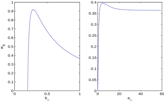
In the Figure 1, we have depicted the adjustment coefficient wR as a function of the retention

level in the case of proportional reinsurance as well as in the case of excess-of-loss reinsurance. In both cases, the graphs suggest that w_R is an uni-modal function of the retention level.

0 0.5 1 0 0.1 0.2 0.3 0.4 0.5 0.6 0.7 0.8 0.9 1 w ℜ b ∞ 0 20 40 60 0 0.05 0.1 0.15 0.2 0.25 0.3 0.35 0.4 a ∞

Figure 1: The adjustment coefficient as a function of the retention level in the case of proportional reinsurance and excess of loss reinsurance respectively

We point out that w_R = 0 when (18) fails (in the classical case when (6) fails). In the propor-tional case (18) is 1 2[1 · b∞+ 2 · 2b∞] > h 1 −4 5 i 1 2[1 · 1 + 2 · 2], i.e. b∞> 0.2. In the excess-of-loss case (18) is

1 2[1 · (1 − e −a∞_{) + 2 · 2(1 − e}−a∞/2_{)] >} h 1 −4 5 i 1 2[1 · 1 + 2 · 2], and, with some easy computations, we obtain

e−a∞/2_{< 2}√_{2 − 2, i.e. a}

∞> −2 log(2

√

Acknowledgements

This work has been partially supported by Murst Project ”Metodi Stocastici in Finanza Matema-tica”. We thank the referee for some valuable comments and suggestions which led to an improve-ment of both the content and the presentation of the paper.

References

[1] Baldi P. and Piccioni M., A representation formula for the large deviation rate function

for the empirical law of a continuous time Markov chain, Statist. Probab. Lett. 41 (1999),

107–115.

[2] Borovkov A.A., Boundary values problems for random walks and large deviations for

func-tion spaces, Theory Probab. Appl. 12 (1967), 575–595.

[3] de Acosta A., Large deviations for vector valued L´evy processes, Stochastic Process. Appl. 51 (1995), 75–115.

[4] Dembo A. and Zeitouni O., Large Deviations Techniques and Applications, Jones and Bartlett, Boston 1993.

[5] Duffield N.G. and O’Connell N., Large deviations and overflow probabilities for a single

server queue, with applications, Math. Proc. Camb. Phil. Soc. 118 (1995), 363–374.

[6] Hald M. and Schmidli H., On the maximisation of the adjustment coefficient under

pro-portional reinsurance, Astin Bull. 34 (2004), 75–83.

[7] Hipp C. and Vogt M., Optimal dynamic XL reinsurance, Astin Bull. 33 (2003), 193–207. [8] Macci C., Stabile G. and Torrisi G.L., Lundberg parameters for non standard risk

processes, Scand. Actuarial J. 2005, n. 6, 417–432.

[9] Macci C. and Torrisi G.L., Asymptotic results for perturbed risk processes with delayed

claims, Insurance Math. Econom. 34 (2004), 307–320.

[10] Rolski T., Schmidli H., Schmidt V. and Teugels J.L., Stochastic Processes for

Insur-ance and FinInsur-ance, Wiley, Chichester 1999.

[11] Schmidli H., Optimal Proportional Reinsurance Policies in a Dynamic Setting, Scand. Ac-tuarial J. 2001, n. 1, 55–68.

[12] Schmidli H., Asymptotics of Ruin Probabilities for Risk Processes under Optimal

Reinsur-ance policies: the Small Claim case, Working Paper 180, Laboratory of Actuarial

Mathemat-ics, University of Copenhagen (2004).

[13] Schmidli H., Asymptotics of Ruin Probabilities for Risk Processes under Optimal

Reinsur-ance and Investment Policies: the Large Claim case, Queueing Systems 46 (2004), 149–157.

[14] Waters H.R., Some mathematical aspects of reinsurance, Insurance Math. Econom. 2 (1983), 17–26.