NEW FORMALISM FOR PRODUCTION SYSTEMS MODELING
Guido Guizzi(a), Daniela Miele(b), Liberatina Carmela Santillo(c), Elpidio Romano(d)
(a), (b), (c), (d) University of Naples “Federico II”, Naples – Italy
(a)[email protected], (b)[email protected], (c) [email protected], (d) [email protected]
ABSTRACT
This paper aims to highlight the usefulness of the simulation, analyzing in particular, two simulative techniques: the Discrete Event Simulation and the System Dynamics. The main objective is to propose a simulation methodology to use to model, analyze and control any type of system. This approach is supported by three studies, belonging to different sectors, which demonstrate the utility of adopting a simple and common scheme of analysis.
Keywords: Simulation, Decision making, System Dynamics
1. INTRODUCTION: THE SIMULATION The simulation is a methodology for experimental analysis of dynamical systems and in particular of complex dynamic systems.
The term "system" refers to a set of entities that, individually distinct, interact through interdependent relationships or reciprocal connection (Forrester 1961).
The systems in question are dynamic: they are characterized by the evolution over time. The emphasis is placed not only on the analysis of the system as a state of equilibrium, but focuses on the process through which change over time. Technically, the dynamics of a system is defined as the succession of its states over time, where the system state is a set of measurable quantities. The further attribute is the complexity. A complex system has its own characteristics, which do not correspond to the sum of the parts that constitute it. In other words, the network of relationships between entities produces non-linear effects that can’t be explained by studying each component separately (Bertalanffy 1969).
Therefore, the presence of non-linearity, dominant feature in complex systems, leads to adopt the simulation as interesting alternative to analytical models in the study of complex dynamic systems.
The simulation is a methodology that is part of the so-called experimental mathematics. It is a representation of the system, realized through a computer language, which allows to use the computer to calculate numerically the behavior. This methodology provides a valid alternative analysis: "The simulation models thus represent a significant response to the demands of flexibility and adaptability descriptive, on
the one hand, and of the possibility of computation, on the other. A computer code has formal, adaptability and flexibility and computability requirements."
The adaptability of the simulation is referring to the fact that the programming languages allow to define the properties of the system in great detail, determining the behavior dynamically, based on its current state. Through the conditional constructs, typical of programming languages (if ... then ... else), it is possible easily introduce such behaviors conditionals in simulation models. There are also disadvantages: the simulation implies difficulty in generalizing the results. For example, the task to extract general rules from a simulation model is more difficult compared to the case in which these rules must be extracted from an analytical model. In fact, in the analytic case, the solution of the equation system allows you to have full information on the system represented. While the simulation is only able to provide information relating to particular demands of the possible future path of the model, often determined by the initial parameters. This methodology does not promise to deliver the same quality and information content of an analytical solution, but certainly allows to analyze and formalize complex systems, otherwise intractable.
2. THE SIMULATION TECHNIQUES MOST WIDESPREAD
Below, there are the two most common techniques of numerical simulation based on the computer:
§ The Discrete Event Simulation (DES); § The System Dynamics (SD).
Each of them is characterized by a specific formalism for the representation of the entities, relationships and time
2.1. The Discrete Event Simulation (DES)
The Discrete Event Simulation is based on a dynamic ordering of events in time. The system evolves through a succession of leaps in time, at which an event occurs and changes the status of the system. The discrete event simulation is based on a dynamic ordering of events in time (Caputo, Gallo and Guizzi 2009; Guerra, Murino and Romano 2009).
Certain events are scheduled at the beginning of the simulation, others are generated during execution. The simulated experiment consists in the reproduction
sequence of status changes. This simulation methodology is very useful for analyzing the utilization rate of resources (production units) and to highlight the eventual critical points (bottlenecks) in the process (Gallo, Montella, Santillo and Silenzi 2012).
This methodology adopts a graphic symbols. The processes are sequences of activities described by graphic symbols, linked by sequential relationships (the lines connecting them). The entities, said token, flow within the chain described by the process. The token is a placeholder that moves in the process and occupies the possible queues. The token is a placeholder that moves in the process and occupies the possible queues. In addition to the token, also the information can flow. So, through a different symbology, it is possible to distinguish the routes taken by the information and those made by the token. For each token may be associated state variables that are normally handled by the units. Thanks to the graphical representation and the rich library of symbols (building block), available in a discrete event simulator, it is possible to construct models with a reduced use of programming. The adoption of programmable blocks allows to realize sophisticated models with relative simplicity and clarity of expression. Such logic design is similar to that used to draw the electronic circuits. Employing the integrated circuit, capable of performing complex functions, it is possible to construct a complicated circuit by adopting a scheme very simple.
2.2. The System Dynamics (SD)
Among the techniques of simulation, this is the one that is closest to the mathematical formalism, in fact, is based on differential equations. The system dynamics is based on a useful perspective to represent the relations of cause and effect in the dynamic phenomena (Revetria, Catania, Cassettari, Guizzi, Romano, Murino, Improta and Fujita 2012). Compared to other simulation techniques, it enables a reduced use of programming languages, allowing extreme rapidity in the design of the models. In the formalism of system dynamics, there are three types of variables:
§ the level variables (also called stocks); § the flow variables;
§ the auxiliary variables.
The Level variables relate to stock or endowment of a good at a given time t, acting as containers that are filled and emptied during the evolution of the system. The flow variables represent the rate with which a variable level changes over time. The net rate of change of a stock is the sum of all inflows minus the sum of all the outflows. Mathematically, the stock integrate their net flows, while the net flow is the derivative of the stock. Obviously the rate represented by the flow variables can be expressed as a constant value, a function stochastic or can depend on other variables of the model.
Another fundamental element for the System Dynamics is the delay. The delays are divided into two categories:
§ The material delay. It postpones the flow of goods in output from a variable level, ensuring that the total of what enters the stock is equal to the total of what will come out; § The delay of information. It does not guarantee
that the sum of the information in input is equal to that in output. In the cognitive process, in fact, the most recent information may overlap with those previously perceived. The System Dynamics uses two types of diagrams, useful in describing the system in analysis:
§ The Causal Loop Diagram, which allows to represent in a direct way the system from the mere point of view of the relations of cause and effect;
§ The Stock and Flow Diagram, which allows to represent the system as a function of the variables of stock, the flow variables and auxiliary areas.
2.3. SD vs DES
The SD and DES are two basic simulation techniques, both used as a tool for decision support and therefore, both adopted to analyze the evolution of the system over time and its behavior according to the variation of some parameters.
In fact, there are substantial differences in terms of modeling approaches: the SD traces the problem, on the basis of its general structure, emphasizing the causal links between the variables, while the DES attempts to trace the path followed not by the system, but by a single element forming part of it.
The table I presents a clear overview on the aspects that characterize and differentiate the two approaches.
The SD models are adopted to study complex systems and offer the possibility to aggregate a large number of individual objects in the flows. The SD allows the evaluation of the behavior of the system for long periods of time, responding to the needs especially strategic (Converso, De Carlini, Guerra and Naviglio 2012; Gallo, Aveta, Converso and Santillo 2012). While the DES, is usually adopted to model business processes, which require specific performance measures, such as the levels of production output or levels of customers served (Gallo, Guerra, Guizzi and 2009).
Stahal (1995), in his studies, shows that, due to the high level of aggregation, the models in SD, tend to be relatively small in terms of number of elements considered, on the contrary, the models in DES tend to be rather complex, as each process is modeled in detail, until the single working units. The level of detail, then, in DES, is a critical factor: a very detailed model takes a long time to realize it and may be less reliable. The first step to define a pattern in DES is the mapping of the process, through which to define logical relationships among the elements. The mapping process, realized according to the logics of DES, may be sufficient to understand the system, without necessarily proceed with the simulation. The DES, as previously mentioned, it is
appropriate to conduct a detailed analysis of a specific system, that is well defined and linear, so as to provide estimates of performance measures statistically valid, such as the number of entities or pieces in the queue (Greasley, 2009). The previous statements confirm the choice of System Dynamics, as a simulation tool for the study of the behavior of a flow shop, whose production follows the logic of the Make to Order, according to the priority rule FIFO. Furthermore, the deficiency, in the literature, of similar works, compared to DES in studies on production systems, has led again to make use of the System Dynamics to conduct the work mentioned.
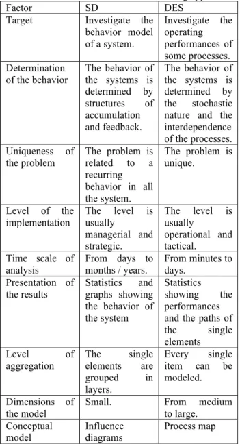
Table 1: Criteria for selection of modeling approach
Factor SD DES
Target Investigate the behavior model of a system. Investigate the operating performances of some processes. Determination of the behavior The behavior of the systems is determined by structures of accumulation and feedback. The behavior of the systems is determined by the stochastic nature and the interdependence of the processes. Uniqueness of the problem The problem is related to a recurring behavior in all the system. The problem is unique. Level of the implementation The level is usually managerial and strategic. The level is usually operational and tactical. Time scale of analysis From days to months / years. From minutes to days. Presentation of the results Statistics and graphs showing the behavior of the system Statistics showing the performances and the paths of the single elements Level of aggregation The single elements are grouped in layers. Every single item can be modeled. Dimensions of the model
Small. From medium
to large. Conceptual model Influence diagrams Process map
3. METHODOLOGICAL SCHEME FOR THE SIMULATION IN SD
The core of this paper is to describe a methodology to schematize, analyze, manage and control a process of every kind, whether belonging to the manufacturing world and the service sector, in an optimal manner (Guizzi, Chiocca and Romano 2012; Guizzi, Murino and Romano 2012). After a long and careful study path
it was possible to observe that the reality can be easily schematized through the aid of three elements. This means that in any type of system it is possible to find three basic tools, which allow the dynamic developments control of the same. The items under discussion are as follows:
§ A time system, the Hourglass;
§ A system of evolution, the Chain of Events; § A system of routing, the Route.
The Hourglass is the time constraint that the system under analysis must respect. An hourglass has the function to mark the time to perform a given operation. When the time runs out, the operation is considered ended and only then, eventually, if all other constraints have been met, the entity can move to the next stage. The schema of the hourglass is characterized by a variable level "Time object", that increments and decrements itself thanks to flows of input and output, respectively "Load time" and "Unload Time", indicating, for example, the rate at which carries out the operations of loading and unloading. Obviously, the level variable influence some auxiliary variables, such as the "Time Remaining".
Figure 1: Hourglass
The Chain of events is the core of the simulation, through the construction of this it is possible to trigger events that allow the advancement of the entities in the simulation model. The structure is characterized by a variable level "State" that increments and decrements itself thanks to the flows "Shift_in" and "Shift_out", indicating the rate of entry and exit from the particular state.
Figure 2: Chain of events
The Route: the structure is characterized by a variable level, "Route_matrix", through which it is possible to identify the possible routes that entities can undertake.
In order to make clearer the proposed methodology to schematize a system in SD, below it is possible to analyze three different studies conducted with this approach. Specifically, the works just mentioned, regarding the port sector, the airport sector and the productive sector. In these three cases, the system represents the case in which the route is unique and is identified by the chain of events, then all three constitute the case more "trivial."
3.1. Port Model (Guizzi, Santillo and Romano 2013)
A port terminal is a node in the freight network both container and dry bulk. A port terminal is a complex system to manage, in fact inside, often encounter criticality difficult to decipher and to overcome. In this context, there are two types of problems: structural and logistical For example the first type belongs the size of the access channel. The access channel is not the same for each terminal port, otherwise, each channel has its length, but especially its width, depends on the morphology of the place. Obviously an access channel to the terminal with smaller width, presents major complications compared to a channel with a greater width. From the width of the channel depends on the possibility to pass two or more vessels together. The case in which the transit of the channel is constrained to a single ship implies, for example, congestion problems: thus a structural constraint becomes a logistical constraint. Another critical, which has a high complexity, is related to the safety distance, that vessels must maintain between them while they run through the channel. These problems in addition to other difficulties were analyzed by the method mentioned above. In the image below it is possible to observe the chain of events of a port system.
Figure 4: Port Model: Event Chain
The chain of events is the core of the simulation, through the construction of this chain it is possible to trigger events that allow the advancement of the vessels in the circulation model. In this case, the route that the vessels must follow is that indicated by the chain of events and is, therefore, fixed. This means that ships can’t carry out an alternative route. This obstacle is overcome by the introduction of the matrix of routes. This chain of events has been built using the logic of Petri nets and allows to track the movement identified in the context of analysis. In this chain of events, the levels are operations undertaken by the ships in the harbor, from the moment of entry into the channel at the time of exit from the same channel. The flows of the
chain of events represent the different events that must be activated to switch from an operation to the next. The constraints are graphically represented by arrows and must be satisfied so that the events are triggered in the chain and chain operations can proceed. The logic used to trigger the events is of the type "if-then": if the constraints are satisfied, then the event is active, otherwise the event remains inactive until the combination of the constraints is not satisfied. The main constraints related to events, are dimensional constraints and temporal, ie the dimensional constraints are related to the ability of a certain area of the port, such as the quay, to be able to accommodate only a limited number of vessels at the same time because of the limited size of that area, while the timing constraints are represented by the time necessary to make and terminate an operation that precedes a subsequent activity. The timing constraints are represented by means of “hourglasses”, used in such a way as to exhaust the remaining time of a certain task. In this way, only when an hourglass runs out then the system advances to the next step. For example in the case of the operation of maneuver is possible to consider a timing pattern of this type:
Figure 5: Port Model: Time consuming Model in the case of the operation of maneuver
3.2. Production model
The model schematizes a production system "Flow Shop" and the sequencing of its activities, under the rule of dispatching, F.I.F.O. type. The model is composed of two submodels: one for schematize the productive system and one for schematize the sequencing of activities. In this context, the second submodel, just mentioned, is shown. From the figure below it is possible to see the chain of events.
Figure 6: Production model: Event chain The scheme involves a production system "flow shop", consisting of a single production line, where the operations necessary for the realization of products
must be carried out on the same set of machines and in the same order of precedence: the flow of elements along the line is unidirectional and there are precedence constraints between operations. There are four types of product and each of these must be tried on 3 different machines: M1, M2, M3. Each operation will have a different duration by virtue of the product being processed on the specific resource. Furthermore, the machines are "dedicated", then two successive operations must be performed on two different machines. The module respects the following constraints:
§ operations must be specified in the order defined;
§ each machine must perform at most one operation at a time;
§ each operation must be carried out, at most, by a machine at a time, that is, an operation on a machine may commence only after completion of processing on the previous machine.
Upstream of each machine, the module provides a buffer: this means that the buffer downstream of the machine M1 contains the piece, that has been processed by the machine M1, from which it is taken to undergo secondary processing and so on until the end of the process, where there is a buffer of finished products. The levels of the model belong to two categories: some are indicative of the operations that are performed on different machines, others are indicative of the buffer upstream and downstream of a certain resource. The flows, represent the events: to transit from an operation to the next, or from one buffer to another, the constraints must be satisfied, if these are not verified, the event is not activated and the flow does not allow the unit in question to transit from the previous level to the next. In addition, the FIFO rule is implemented: the first element to enter the layer upstream of the chain, will be the first to be worked, and so on all subsequent.
The following constraints were considered: § dimensionless, they are deprived of
measurement units and related to resources; § temporal, they are representative of processing
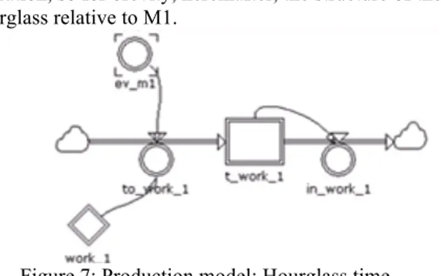
times for each item, on each machine and determine the beginning and the end of the individual machining operations. An item, can pass to a subsequent processing, for example on the machine M2, only if the first machining operation on the resource M1 has been completed: the completion of this operation is defined by a specific level that represents the processing time remaining. The time required to perform each operation is controlled via time constraints: the hourglasses. An hourglass is designed to scan the time to devote to an operation: When the time has run out, the transaction is considered completed and if all other constraints have been met, the product being processed can move on to the next resource to undergo a further processing. The structures of hourglasses, are similar for each type of
operation, so for brevity, hereinafter, the structure of the hourglass relative to M1.
Figure 7: Production model: Hourglass time 3.3. Airport Model
The Airport is an interchange intermodal and can be considered an integrated system of infrastructure, devices and equipment. The operational functionality of airports must be guaranteed by the capacity of its components, which must be dimensioned and must operate at least according to the standard level of work of the airport. In the context of airport operations and structures are usually divided into two areas: “Landside” and “Airside”. The factor that distinguishes these two areas is the capacity: the capacity of the landside is measured in number of passengers served per unit of time, while that of the airside is measured by the number of operations (takeoffs or landings) per unit of time. Between the two subsystems, the airside is the system most likely can generate bottlenecks. This means that this study is focused on the capacity of the airside. In detail, the three sections: the runway, taxiways and parking areas, are in series with each other, so the capacity of the entire subsystem will be equal to the lesser of the three values, and in this regard the critical resource can be runway. The study and implementation of the appropriate measures to increase the capacity of the slopes, however, must not be separated from the consideration of the capacity of the other parts of the system, in order to avoid that these, entering saturation, undermine efforts to increase the capacity of entire airport system. The capacity of a track depends essentially on the distancing between aircraft and the runway occupancy time (landings, takeoffs, or both). In addition, the occupation time of the track employee of the following elements: configuration of the slopes (single, parallel, crossed, etc..), coefficient of utilization of the airport, interference of the slopes between them, the number and location of fast exits from the runway. The airport infrastructure, analyzed, has a single runway, dedicated exclusively to landing operations, in addition, this track is used mainly to the use of aircraft weight class Medium. This infrastructure is also equipped with a Holding Stack consists of a number of circuits equal to 4, arranged at different heights, and such that each circuit can be engaged by only one aircraft at a time. The management of the stack is FIFO type. Thanks to the model created it is possible to identify levels of capacity and delay beyond which the loss of efficiency of the system will reflect itself
negatively on the infrastructure creating congestion. For this purpose, the implementation of an appropriate scheduling for managing the flow of aircraft can make a significant contribution to the increase of efficiency and safety.
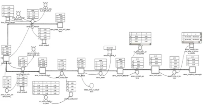
Figure 8: Airport Model: Event Chain
The physical flow of the simulation model precisely describes the path of the aircraft until landing on runway. This flow allows to follow the individual aircraft in all phases that precede the landing: from the descent phase to the landing phase, and then liberation of the track. The FIFO stack implies that the second aircraft, of the waiting sequence in the "stack", can go down to the minimum level only when the first aircraft made free this level and sufficient time to dissipate the turbulence generated is spent. Similarly the subsequent aircraft may descend into the "stack" of waiting to lower levels when these levels were made free from the aircraft above. The aircraft went out from the stack, will have to cross the "final approach path" before starting the landing.
4. CONCLUSIONS
The simulation appears to be a good system of analysis, monitoring and evaluation of real systems, since it offers the possibility to create "experiments" at low cost.
This advantage must be accompanied by a good modeling capabilities, otherwise the simulation approach can be an obstacle to the activities of synthesis and analysis. For this purpose a long process of investigation and study has led to the need to identify a pattern methodological simple and easy to apply for anyone who intends to use the System Dynamics.
The advantage of this approach lies in the possibility to outline and analyze systems of different nature, with the help of three instruments that represent the dynamism of all reality.
REFERENCES
Bertalanffy, V., 1969. General System Theory. New York: George Braziller, pp. 139-1540.
Caputo, G., Gallo, M., Guizzi, G., 2009, Optimization of production plan through simulation techniques,
WSEAS Transactions on Information Science and Applications, 6 (3), pp. 352-362.
Converso, G., De Carlini, R., Guerra, L., Naviglio, G., 2012, Market strategy planning for banking sector: an operational model, Advances in Computer
Science: 6th WSEAS European Computing Conference (ECC '12), pp. 430-435, September
24-26, 2012, Prague, Czech Republic.
Forrester, J., W., 1961, Industrial Dynamics, Pegasus Communications.
Gallo, M., Aveta, P., Converso, G., Santillo, L.C., 2012, Planning of supply chain risks in a make-to-stock context through a system dynamics approach,
Frontiers in Artificial Intelligence and
Applications, 246, pp. 475-496, IOS PRESS.
Gallo, M., Guerra, L., Guizzi, G., 2009, Hybrid remanufacturing/manufacturing systems: Secondary markets issues and opportunities,
WSEAS Transactions on Business and Economics,
6 (1), pp. 31-41.
Gallo, M., Montella, D.R., Santillo, L.C., Silenzi, E., 2012, Optimization of a condition based maintenance based on costs and safety in a production line, Frontiers in Artificial Intelligence
and Applications, 246, pp. 457-474, IOS PRESS.
Greasley, 2009, A Comparison of System Dynamics and
Discrete Event Simulation, Aston Business School,
Aston University, Birmingham, United Kingdom. Guerra, L., Murino, T., Romano, E., 2009, Reverse
logistics for electrical and electronic equipment: A modular simulation model, Proceedings oh the 8th WSEAS International Conference on System Science and Simulation Engineering, ICOSSSE ’09, pp. 307-312, October 17-19, 2009,Genoa, Italy.
Guizzi, G., Chiocca, D., Romano, E., 2012, System dynamics approach to model a hybrid manufacturing system, Frontiers in Artificial
Intelligence and Applications, 246, pp. 499-517,
IOS PRESS.
Guizzi, G., Murino, T., Romano, E., 2012, An innovative approach to environmental issues: The growth of a green market modeled by system dynamics, Frontiers in Artificial Intelligence and
Applications, 246, pp. 538-557, IOS PRESS.
Guizzi, G., Santillo, L.C., Romano, E., 2013, A new model to manage vessels flow in a port Terminal,
7th International Conference on Applied Mathematics, Simulation, Modelling (ASM '13),
January 30-February 01, 2013.
Revetria, R., Catania, A., Cassettari, L., Guizzi, G., Romano, E., Murino, T., Improta, G., Fujita, H., 2012, Improving healthcare using cognitive computing based software: An application in emergency situation, Lecture Notes in Computer
Science, 7345 LNAI, pp. 477-490
Stahl, J., E., 1995, New Product Development: When
Discrete simulation is Preferable to System Dynamics, Elsevier Science.