Rainfall induced instabilities: a field experiment on a silty sand slope in northern Switzerland

Abstract

Two full scale field tests were planned and performed successfully on a steep forested slope located on the east facing banks of river Rhine in Ruedlingen, in canton Schaffhausen, northern Switzerland. The aim of the experiments was to study the triggering mechanisms of the landslides due to rainfall. Intensive field investigations were carried out, including in-situ geotechnical tests, cha-racterisation of hydrological properties of the soil and reinforcing effects of vegetation, geological and hydrogeological mapping, and subsurface investigations by means of geophysical methods. Additionally, several series of saturated and unsaturated laboratory tests were conducted on undisturbed and disturbed samples taken from different depths from the vicinity of the selected slope. The test site was intensively instrumented and monitored over a period of 6 months in the course of artificial rainfall and natural precipitation. The instrumentation includes conventional and novel methods to measure pore water pressure, volumetric water content, piezo-metric height, soil pressure, acoustic emissions, surface and subsurface movements, soil temperature, and meteorological data. This paper introduces briefly the measurements and findings from this multi-disciplinary project, and focuses on numerical and analytical methods used to explain the behaviour of a marginally stable slope before and during the failure induced by rainfall. Simple stability calculations are described that still offer realistic predictions of the status of a slope prone to failure due to increase of the pore water pressure. The basal and lateral reinforcing effects of vegetation and unsaturated shear strength of soil are introduced in these two and three dimensional simulations as well.

1. Introduction

Steep mountainous areas are increasingly en-dangered by natural hazards. Rainfall induced land-slides are one of the major causes of these raised risks. Accordingly, a deeper understanding of the triggering mechanisms of such landslides, and the provision of tools to predict the locations and poten-tial volumes released, is important.

Numerous studies have been conducted to mea-sure the changes in pore water presmea-sure of slopes in response to seasonal and extreme rainfall events. However, few data are available on the hydro-me-chanical behaviour of natural slopes during the fail-ure. Ochiai et al. [2004] summarised four such

ex-periments. Three of them have been conducted in Japan [Oka, 1972; Yagi et al., 1985; Yamaguchi et

al., 1989] and one series of tests was performed by harp et al. [1990] in USA. Ochiai et al. [2004] also

triggered a fluidised landslide by means of artificial rainfall. TeYsseire [2005] mobilised a landslide in the

forefield of the Gruben glacier (Canton Wallis, Swit-zerland).

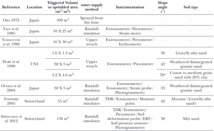
harp et al. [1990] performed three tests on

nat-ural slopes to study the response of the slope to ar-tificial subsurface irrigation in terms of pore water pressure during failure. They induced failure by

ir-rigating the ground artificially through water sup-ply from trenches at the top of the slope and by dig-ging a lower vertical cut, because they had unsuc-cessful attempts to trigger slope failures by sprin-kling with intensities and durations “many times” higher than those of the normal rainfalls. They in-strumented the slopes with piezometers and ex-tensometers. The soil types of each site are sum-marised in table I.

They observed from the lower vertical cut that the water flows, mainly through macropores, dur-ing their experiments (e.g. animal burrows and root casts). However, the flow rates from different pores were not constant during the course of irrigation. The authors reported temporal and spatial change of discharge throughout. harp et al. [1990] also

mea-sured abrupt decreases in the pore water pressure at different locations of the slopes between 5 to 50 minutes prior to failure. They mentioned simultane-ous widening and increase of flow of “muddy water” out of fractures some seconds before failure. They suggest that the raised pore water pressure and in-creased flow might result in redistribution and re-moval of fine particles (piping), which may ultimate-ly lead to increase of the pore sizes and destruction of the soil structure at the shear surface. They con-clude that loss of contact points between the coarser grains can decrease the shear strength of the mate-rial and trigger a landslide.

Ochiai et al. [2004] isolated a 5 m wide and 30

m long experimental slope with an average

gradi-on a silty sand slope in northern Switzerland

Amin Askarinejad,* Francesca Casini,* Patrick Bischof,* Alexander Beck,* Sarah M. Springman*

* Institute for Geotechnical Engineering, Swiss Federal Insti-tute of Technology, ETH Zurich.

ent of 33° (maximum 35°) located on a hill slope, by driving thin steel plates about 1 m deep into the soil. The plates prevented lateral percolation of in-filtrated rainwater and reduced lateral tree root re-inforcement. The surface material on the slope con-sisted of fine weathered disintegrated granite sand. The authors monitored the surface movements of the slope by means of photogrammetry video cam-eras. The depth of the shallow failure surface was de-tected using soil-strain probes, which were installed to a maximum depth of 2 m. The changes in the pos-itive and negative pore water pressures were tracked by means of 6 tensiometers installed in the middle of the slope.

Artificial rain was sprinkled over the selected slope with 78 mm/h intensity for 4.5 hours for the first day, and no movements were measured. This first event was followed after 17 hours by a second one at the same intensity. First slope deformations were observed after 5.5 hours. Slope failure hap-pened approximately 6.8 hours after the sprinkling was commenced. At this moment, a tension crack was observed on top and a compression zone at the bottom of the slope. The landslide liquefied and travelled at a speed of 3 m/s on a 10° gradient. The rate of compression straining in the lower part of the slope was calculated to be greater than the rate of ex-tension straining in the upper part, based on photo-grammetry results.

The tensiometers showed sequential increases in pore pressure according to the installation depth. The shallower tensiometers at depths of 0.50 and 1 m measured increases in pore water pressure and then they showed quite constant values. While, the deeper sensors (>1 m) measured sudden increas-es after the water front reached the corrincreas-esponding depth and pore pressure did not attain a steady state condition with continuous increase until the final failure. This behaviour was attributed to the effect of the isolating longitudinal plates. However, it could also be an indication of the existence of preferen-tial water paths in the shallower soil strata. The au-thors of the paper point to the coincidence of the arrival of the wetting front to the lowest tensiometer (depth of 2.90 m) with the acceleration of the bend-ing strain at the depth of 1.10 m about 2 hours be-fore the failure. This observation can be explained by the fact that the lowest tensiometer is installed at the interface of the soil mass and the bedrock, and arrival of the wetting front at this level might result in development of perched water table, which might favour further increase of the pore water pressure at shallower depth [kienzler, 2007]. This hypothesis

could be supported by the change in rate of increase in pore water pressure measured by the tensiometers at depth of 1.0 and 1.5 m (which are installed near the eventual shear surface), approximately 2 hours before the failure.

Tab. I – Landslide triggering experiments on natural slopes [modified after Ochiai et al. 2004].

Tab. I – Frane superficiali su pendii naturali [modificata dopo Ochiai et al. 2004]. * The value is deduced based on the contours on the plan view.

Reference Location Triggered Volume or sprinkled area (m3_/m2₎ water supply method Instrumentation Slope angle (°) Soil type

Oka 1972 Japan 500 m3 Sprayed from

fire hose -

-Yagi et al.

1985 Japan 10 X 25 m2 simulatorRainfall Extensometer/Piezometer/Strain meter - -Yamaguchi

et al. 1989 Japan 10 X 30 m2 Upper trench Extensometer/Piezometer/Inclinometer -

-harp et al.

1990 USA

1.6 X 1.3 m2

Upper

trench Extensometer/Piezometer

30 Gravelly silty sand

30 X 5 m2 ₄₃ Weathered disintegrated

granite sand

3.2 X 4.0 m2 _{70* Coarse to medium grain}

sand with 20% clay Ochiai et al.

2004 Japan 30 X 5 m2 simulatorRainfall

Extensometer/ Tensiometer/Strain probe/ Photogrammetry 33 Weathered disintegrated granite sand TeYsseire

2005 Switzerland 55 m2 simulatorRainfall TDR/Tensiometer/Moisture point 42 Moraine (Gravelly silty sand) springman et

al. 2012 Switzerland 130 m3 simulatorRainfall

TDR/Tensiometer/ Piezometer/Soil deformation probe/ERT/

Soil pressure sensors/ Photogrammetry

TeYsseire [2005] selected a 42° steep alpine

mo-raine slope, at about 2800 m above sea level (masl) in the forefield of the Gruben glacier (Canton Wal-lis, Switzerland) as a field test site. It was instrument-ed over a 55 m2 _{plan area for an artificial rainfall test} in summer 2000, to investigate slope stability in mo-raine as a function of degree of saturation and rela-tive density of the soil.

A series of insitu direct shear box tests, of plan area 250 mm x 250 mm, was carried out at the field test-site on samples that were carved out of the un-saturated ground. The specimens exhibited dilatan-cy at failure. The internal friction angle for this soil, based on the gradient of the peak shear strength en-velope, was j′ = 41° [springman et al., 2003].

Rainfall was applied for 50 hours with an average intensity of 16 mm/h for the first day and 12 mm/h for the second day. The slope failed after ~2 days, and the sprinkling was stopped. Instability occurred in the slope when Sr approached 0.95. The slip sur-face was located at the depth of approximately 0.2 m. Time Domain Reflectometers (TDRs) installed at depths of 0.19 and 0.12 m show a decrease in the de-gree of saturation at approximately 6 and 1.5 hours before the failure, respectively. This observation is similar to the results of harp et al. [1990] and can be

attributed to the dilation of the soil elements along the shear surface. This hypothesis might be support-ed by the fact that the drop in the degree of satu-ration measured at depth of 0.19 m, which is the nearest sensor to the failure surface, was more pro-nounced [askarinejad et al., 2010b].

alOnsO et al. [2003] performed a series of

cou-pled hydro-mechanical simulations to analyse the be-haviour of an instrumented unstable slope in east-ern Italy in terms of slope motions, variation of safe-ty factor, and their relationship with rainfall. The in-vestigated slope is composed of three partially sat-urated overconsolidated clay layers. The authors showed that changes between layers might result in high pressures at the interfaces of layers. These peak pressures decrease the factor of safety and enhance the strains. Accumulated strains might promote the strength degradation lead to movements develop-ping at the interfaces. Accordingly, they lead to con-clude that the hydraulic properties of the soil profile play a major role in the stability of layered slopes.

ng and shi [1998] performed a parametric study

using finite element method to analyse the stabili-ty of unsaturated slopes due to rainfall. They found out that not only the intensity of the rainfall event, but also the initial ground water level and duration of the rain play, major roles on the stability of the slopes.

Despite prior research, there is still a lack of knowledge on some aspects, such as the stabilis-ing effects of vegetation, the influences of bedrock shape, the regional hydrogeological properties, and

all are linked to the hydro-mechanical behaviour of the overlying unsaturated soil.

This project was conducted within the context of a multi-disciplinary research programme on Trig-gering of RApid Mass Movements in steep terrain (TRAMM1_{). The primary focus of this research is to} enhance the understanding of triggering and initia-tion mechanisms, including the transiinitia-tion from slow to fast mass movement processes, and flow character-istics of such catastrophic mass movements. The influ-ence of rainfall events on slope stability is investigated by monitoring a natural slope in Ruedlingen, Switzer-land. The hydro-mechanical responses of the slope were studied under natural and artificial atmospheric conditions. These results are used to calibrate models adopted to predict possible landslides in the future.

The characteristics of the experiment field in terms of the topography, geology and hydrogeology and the shape of the bedrock, hydrological proper-ties of the soil mass, the instrumentation plan and the saturated and unsaturated hydro-mechanical properties of the soil are discussed. The responses of the slope to two intense artificial rainfall events (October 2008, and March 2009) are discussed next. The first experiment, (October 2008) despite having a more intense rainfall and longer duration, did not result in triggering a landslide. However, in the second experiment (March 2009) a landslide of 130 m3 _{was mobilised after 15 hours of rainfall. The} difference between the two experiments was in the location of the rain concentration (rain was more intense at the places were the bedrock was shallow-er and less vegetation effects wshallow-ere expected in the second experiment). In the next section of the pa-per, simplified 2 and 3 dimensional limit equilibri-um methods are implemented to investigate the ef-fect of the side walls of the failure wedge and also the roots reinforcement on the changes of the fac-tor of safety of a slope subjected to rainfall. Finite element program was used to simulate the changes in the pore water pressure during the rainfall and the results are compared to the in situ measure-ments. The effects of the vegetation on the evolu-tion of the factor of safety are also studied.

2. Experiment field

The experiment field was chosen in a forested area near Ruedlingen village, which is located in northern Switzerland. Following an extreme event in May 2002, in which 100 mm of rain had fallen in 40 minutes, 42 surficial landslides occurred around the local area [Fischer et al., 2003]. The selected

experimental site of 35 m length and 7.5 m width is a small part of a slope on the east facing bank along the river Rhine. Figure 1 shows the location of the test site and previous landslides. The altitude is about 350 masl. The average gradient of the slope was determined using a total station theodolite to be 38° with maximum of 43° in the middle of the slope. The surface of the slope is slightly concave; the longitudinal centreline is 0.3 to 0.5 m lower than the sides (Fig. 3).

2.2. Geology and the bedrock shape

The site is located in the Swiss lowlands. The geological progression consists mainly of Molasse, which is the sediment that was deposited in the

fore-land basin of the Alps, containing alternate deposi-tions in the Tethys Sea (Seawater Molasse) and on land (Freshwater Molasse) (Fig. 2). Several bore-holes, as well as an outcrop of bedrock about 20 m above the selected field, revealed horizontal layering of the sedimentary rocks at the experimental slope, which consisted of fine grained sand- and marlstone [Tacher and lOcher, 2008]. Fissures with openings

of more than some centimetres in size were mapped in the lower freshwater molasse, and were parallel to the Rhine [Brönnimann et al., 2009].

Dynamic probing tests were performed every 2 m around and across the middle of the field in order to locate the depth of bedrock. The probing was do-ne with the Dynamic Probing Light method (DPL), which operates with a 10 kg weight, dropped over 0.5 m, generating energy of 50 kJ to drive rods and a cone into the ground. The cone diameter is d = 35.7 mm (cross section: 1000 mm2_{), tip angle 90° [DIN} 4094]. The penetration rate of the cone allows the mechanical resistance of the soil to be evaluated em-pirically. The number of required blows for each 0.1 m was counted, and the criterion for the underlying bedrock was set as 30 blows per 0.1 m penetration.

According to the DPL results, the bedrock lev-el lies between 0.5 m to more than 5 m depth. Bed-rock on the right hand side of the field (P3-M2-P4) is shallower than on the left (P2-M1-P1; Fig. 3). The shallow convex feature located between M1-M2 and P1-P4 may be due to the accumulation of older land-slide materials. The gradient of the slope is about 25° at this point.

These results agree well with those obtained from extensive geophysical Electrical Resistivity To-mography (ERT) surveys [gamBazzi and suski, 2009],

although post slide excavation revealed the presence of stones embedded in the matrix of the overlying soil (possible former debris), which could have im-plied that bedrock had been reached at a shallower depth than was actually the case.

Fig. 1 – Location of the test site, detailed map and map of Switzerland [after sieBer, 2003].

Fig. 1 – Ubicazione del sito di prova, mappa dettagliata e mappa della Svizzera [da Sieber, 2003].

Fig. 2 – The geological lithology of the test site [after Brönnimann et al., 2009].

Electrical Resistivity Tomography (ERT) provides a tool for measuring and high quality imaging elec-trical resistivity in soil. Decreases in the elecelec-trical re-sistivity during a rainfall event can be due to increas-es in the degree of saturation. ERT measurements were performed along the left and right longitudi-nal sections of the slope in the first experiment in October 2008, and March 2009, respectively [lehm -ann et al., 2012]. The ERT measurements were

con-ducted every 30 minutes during the artificial rainfall events applied in both experiments. The

consider-able changes in the resistivity (from more than 140 ohm.m to 20 ohm.m) at some localised points in the bedrock during the course of the rainfall can be an indication of the location of fissures. Several fissures in the bedrock have been recognised based on hy-drogeological investigations before the monitoring experiment and tracking the changes of the electri-cal resistivity of the slope during the experiment. 2.3. Hydrology

Three sets of combined sprinkling and dye trac-er tests wtrac-ere ptrac-erformed at difftrac-erent locations near the experiment slope to characterise the hydrolog-ical properties of the soil profile [kienzler, 2007].

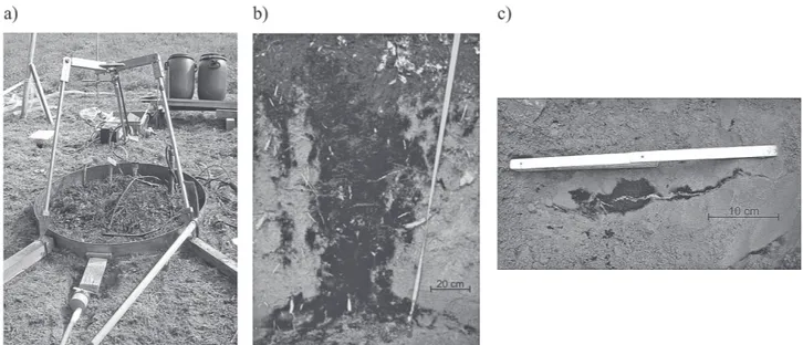
These tests were done through sprinkling dyed wa-ter with uniform intensity of 60 mm/h over a con-fined circular area of 1 m2 _{(Fig. 4a). Runoff was} mea-sured using a 100 ml tipping bucket. Brilliant Blue FCF food dye was added in a concentration of 4 g l-1 to the sprinkling water to visualise infiltration flow paths [springman et al., 2009]. Three vertical sections

with spacing of 0.15 to 0.2 m, and depth of 1.2 m were excavated about 24 hours after the sprinkling had stopped.

Dye patterns (Fig. 4b) were analysed accord-ing to Weiler and naeF [2003]. The dye patterns

showed a mixture of preferential drainage along the roots combined with more homogeneous wet-ting in some locations. Evidence was noted of par-tial perched saturation above the sandstone bed-rock. However, stained fractures below the sub-soil (Fig. 4c), revealed that substantial drainage

Fig. 3 – The 3D shape of the bedrock based on DPL results.

Fig. 3 – Mappa 3D del substrato roccioso in base ai risultati DPL.

Fig. 4 – a) Small-scale sprinkling apparatus for the combined sprinkling and dye tracer experiments; b) Dye pattern; c) Stai-ned fracture in the weathered bedrock below the subsoil [springman et al., 2009, photos: P. Kienzler].

Fig. 4 – a) Attrezzatura utilizzata su piccola scala per le prove di pioggia artificiale costituita da fluido colorante blu; b) Percorso del colorante; c) Frattura nel substrato roccioso raggiunta dal fluido colorante [springman et al., 2009; photo: P. Kienzler].

might occur into the bedrock, which may prevent complete saturation and failure of the experimen-tal slope [kienzler, 2008]. No runoff was observed

during the sprinkling at any of the three locations [springman et al., 2009].

2.4. Instrumentation

The slope was instrumented to monitor the hy-drological and geo-mechanical responses of the soil and bedrock during the rainfall events. Detailed measurements of positive and negative pore water pressures (using tensiometers), piezometric water level (using piezometers) and soil volumetric water content (using TDRs), subsurface flow and runoff were performed. Deformations were monitored dur-ing the experiment, both on the surface usdur-ing pho-togrammetrical methods and within the soil mass, using a flexible inclinometer equipped with strain gauges at different points and two axis inclinometers on the top [askarinejad, 2009].

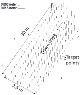
The instruments were installed mainly in three clusters over the slope. Each cluster included a soil temperature sensor at depth of 0.6 m, deformation probes, earth pressure cells, acoustic sensors and rain gauges (Fig. 5). The tensiometers were installed at depths of 0.15, 0.3, 0.6, 0.9, 1.2, and 1.5 m in each cluster and were collocated, as much as possible at each depth, with TDRs at 0.15 m, and from 0.3 m to 1.5 m, with a spacing of 0.3 m.

All the instruments were calibrated and checked in the laboratory that they functioned correctly be-fore installation in the field. The hydrological

re-sponse of the soil was measured during the exper-iment with a logging interval of 5 minutes, while the subsurface deformations and the horizontal soil pressures were measured at a frequency of 100 Hz.

The artificial rainfall was applied by means of 10 sprinklers located at the same spacing on the mid-dle longitudinal line of the field in the first experi-ment (Fig. 5). Lower sprinklers experienced high-er hydraulic heads as wathigh-er was supplied from above the slope and so rainfall was not uniformly distribut-ed. The rain intensity at the lower part of the slope (where larger fissures were detected and bedrock was deeper) was higher than at the top of the slope.

Accordingly, the sprinklers were rearranged for the second experiment. The spacing between the lower sprinklers was increased and 4 more sprinklers were added to provide more rainwater to the upper part of the slope where less root reinforcement and shallower bedrock was expected (plan view in Fig. 5).

3. Soil characterisation

3.1. Soil classification

Soil samples were collected from test pits (TPs) at different depths. The grain size distribution, the natural water content, together with consistency lim-its and activity, are shown with depth for the time of sampling for TP1 in the upper part of the slope. The data for TP1 may be considered to be representative of the whole test site.

The soil can be classified as medium to low plas-ticity silty sand (ML) according to USCS. Activity of

Fig. 5 – The bedrock topography and the instrumentation plan [askarinejad et al., 2010b].

the soil is derived from the chloritic-smectitic clay fraction [cOlOmBO, 2009]. The activity, I_A, is higher

than 1.25 in the upper part of the soil profile and de-creases from IA = 1.25 to IA = 0.75 below 1 m depth. The clay fraction increases with depth from 4% at shallow depths to 10% at about 2 m. The silt fraction also increases with depth from 25% to 32%, while the sand fraction decreases from 67% to 56% (Fig. 6). The increase of the fine fraction with depth may be due to internal erosion induced by sedimento-logical and morphosedimento-logical reasons, and downward transport promoted by infiltrating water, flushing the fines into the larger voids surrounding the peds [casini et al., 2010a].

As the relevant properties of the soil are most-ly influenced by the fines content, undisturbed sam-ples from different depths, with various fines con-tent, were tested in the laboratory experimental pro-gramme presented in the following section [casini et

al., 2010a].

3.2. Laboratory tests

An extensive soil investigation was conducted to understand how the strength is mobilised in the soil and how this may be related to change in water con-tent and void ratio in the slope. The investigation in-cludes tests on both undisturbed and reconstituted soil samples. Water retention characteristics and hy-draulic conductivity have been investigated. Oedom-eter tests, in situ shear tests, laboratory tests with a standard shear and a modified shear apparatus have been performed as well as triaxial tests on saturated and unsaturated soil samples [springman et al., 2009;

cOlOmBO, 2009; casini et al,. 2010 a-b].

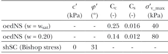
The parameters obtained from oedometer tests on natural samples (oedNS) and shear tests on stati-cally compacted samples (shSC) are summarised in Table II.

Tab. II – Parameters obtained from laboratory results.

Tab. II – Parametri ottenuti dalle prove di laboratorio.

c′ (kPa) j′ (º) Cc (-) Cs (-) s′v_max (kPa) oedNS (w = wsat) - - 0.25 0.016 40 oedNS (w = 0.20) - - 0.14 0.012 80 shSC (Bishop stress) 0 31 - - -3.2.1. TriaxialTesTs

Isotropic and anisotropic drained compression tests were performed to different stress ratios, both to replicate the in situ stress state and to analyse the dependence of volumetric stiffness on the stress ratio [casini et al., 2010a]. After volumetric compression,

failure was approached following a range of suitable stress paths under different drainage conditions.

Standard drained (CIDC) and undrained (CI-UC) shear compression tests were performed, to-gether with constant axial load shear compression tests under decreasing isotropic stress due to the in-crease of pore water pressure. In the latter case, both drained (CADCAF) and undrained (CADCAUF) conditions were studied after an initial drained stage, to analyse the influence of the hydraulic boundary conditions on the eventual failure mechanism of the soil specimens [casini et al,. 2010a]. The data

collect-ed are reportcollect-ed in terms of:

p′ = 1/3 (sa + 2sr); q = sa – sr; p′ = p – u; h = q/p′; (1)

Fig. 6 – Basic properties with depth : (a) Grain size distribution ; (b) Gravimetric water content, Atterberg limits and plasti-city index ; (c) Activity index (after casini et al., 2010a).

Fig. 6 – Proprietà di base con la profondità: (a) Distribuzione granulometrica; (b) Contenuto gravimetrico d’acqua, limiti di Atterberg e indice di plasticità; (c) Indice di attività (da caSini et al., 2010a).

eq = 2/3 (ea – er); ev = ea +2er; Du = u – u0 (2) where sa is the axial total stress and sr is the

radi-al totradi-al stress applied in the triaxiradi-al cell under axi-symmetric conditions. Pore water pressure u is mea-sured in both the upper and lower platens, u0 is the

initial pore water pressure. Axial strain is defined as ea = Dh/h0 where h0 is the initial height of the speci-men prior to shearing and Dh was measured over the entire specimen length. Volumetric strain ev = DV/V0 was deduced from water exchange into or out of the specimen, where DV is the volume change and V0 is the corresponding initial volume prior to

shearing. Conventionally, radial strain was derived as er = (ev – ea)/2. Deviatoric stress is defined as q = sa – sr = F/A, where F is the axial force and A is the current cross-sectional area of the specimen, cor-rected by assuming it remained as a right cylinder [head, 1998].

The results for the CIDC and CIUC tests, plot-ted all together in the eq – h plane, were exploited

to detect a possible critical state stress ratio. In spite of the data variability, typical of natural samples, a value of hCS = 1.30, corresponding to a critical state friction angle of about j′cs = 32.5°, seems to repre-sent the critical state conditions for this soil. The CADCAF results are reported in figure 7. Specimens TX9 and TX10 were anisotropically compressed un-til to p′ ≈ 100 kPa with h = 0.95 and h = 0.44 respec-tively. Increasing the pore water pressure promotes a slight increase in the void ratio for TX9, which is likely to be the result of elastic swelling as the stress path moves inside the yield locus. Slightly after the critical state stress ratio, a definite increase in shear strain was observed, together with a further sudden increase in volumetric strain. The data, which will be discussed in more detail in the following section,

al-ready highlight the stress ratio (e.g. h = q/p′ ≥ 1.4) at which an instability mechanism occurred. The sud-den increase in volume is the evisud-dence of a dilatant failure mode with plastic volume increase.

The difference in friction angle between shear tests (statically compacted sample) and triaxial tests (natural sample) may be due to the different type of test [nOcilla et al., 2006; han and VardOulakis,

1991].

3.3. Saturated and unsaturated hydraulic conductivities The hydraulic conductivity measurements are carried out based on the instantaneous profile meth-od [daniel, 1982]. This method consists of

measur-ing the variation of the suction and volumetric wa-ter content profile within an infiltration column as a function of time during the infiltration process. Ac-cordingly, an infiltration column was developed with a height of 600 mm and an inner diameter of 170 mm. The suction and volumetric water content were measured simultaneously every 100 mm in depth by 3 mm diameter tensiometers and TDRs, respective-ly. These measurements provide enough data to cor-relate the hydraulic conductivity with the negative pore water pressure and/or degree of saturation. The change in the height of the soil sample during the flow of water is monitored using a set of LVDTs on the upper part of the soil column, enabling the volumetric changes to be tracked during the test. The tests are performed on statically compacted soils with different initial void ratios. The configuration of the tests is illustrated in figure 8.

Based on Darcy’s law (Eq. 3), the hydraulic con-ductivity k is calculated by dividing the water flow ve-locity by the hydraulic gradient.

0

50

100

p' (kPa)

0

50

100

q (kPa)

0

10

20

30

ε

(%)

0.5

0

-0.5

-1

-1.5

-2

ε

(%

)

0

5

10

(a)

(b)

Fig. 7 – CADCAF results: (a) p’-q plane; (b) eq – ev plane, with strain axes at the top for TX10 and bottom for TX9 [casini et

al., 2010a].

k = – v_i (3)

where k is the hydraulic conductivity (m/s), v is the velocity of water flow (m/s) and i is the hydraulic gradient.

The water flow velocity v is defined as the vol-ume of water flow passing through the whole cross-sectional area over a given time increment (Eq. 4):

v = Vw ₍₄₎

ADt

where A is the cross-sectional area (m2_{) of the} in-filtration column, Vw is the volume of water

flow-ing through the column (m3_{) and Dt is the time} re-quired for the flow (s).

Combining equations (3) and (4), the unsaturat-ed hydraulic conductivity can be calculatunsaturat-ed basunsaturat-ed on the measured pore water pressure and changes in the profile volumetric water content.

k = Vw

(5) ADti

The hydraulic gradient (i) can be calculated us-ing Equation (6) for an upward water flow.

ii = (Hp,i + He,i) – (Hp,i + 1 + He,i + 1) =

(6) Dz

= (Hp,i – Hp,i + 1) Dz

where, ii is the hydraulic gradient at point i, Hp,i is

the pressure head at point i, He,i is the elevation head

of point i and Dz is the vertical distance between the

points i and i+1. Accordingly, the suction profile in the soil is needed in order to calculate the hydraulic gradient between different elevations.

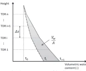
The volume of water passing through any cross-sectional area over a given time increment is equal to the change in the volume of water occurring be-tween the point i under consideration and the top of the specimen (Fig. 9). This volume can be calcu-lated using a trapezoidal rule based on the volumet-ric water contents measured by the TDRs at different heights between two different times:

Vw = A

Σ

(

)

and time j, and n is the number of TDRs.

The changes in the pore water pressure and vol-umetric water content are measured simultaneously during these tests and a water retention curve could be derived, based on these results (Fig. 10a).

The saturated conductivity is measured to be about 10-6 _{m/s (Fig. 10b). This value is lower than} the in-situ measurements of hydraulic conductivity performed using the inversed auger-hole method [OOsTerBaan and nijland, 1994]. The in-situ

mea-sured hydraulic conductivity varies between 10-4 _to 10-5 _{m/s [Brönnimann et al., 2009]. The} inconsis-tency between the laboratory and in situ measure-ment can be explained by the influence of the dif-ference in micro- and macro-porosities in the re-constituted soil and the natural soil. The hydraulic conductivity of Ruedlingen soil decreases by two orders of magnitude with 40 kPa increase in the suction (Fig. 10b).

Fig. 8 – Infiltration column (dimensions in mm).

Fig. 8 – Colonna di infiltrazione (dimensioni in mm).

Fig. 9 – Schematic of water content distribution through the infiltration column.

Fig. 9 – Rappresentazione schematica della distribuzione del contenuto in acqua nella colonna di infiltrazione.

4. Slope monitoring experiment

The applied rain intensity is shown in figure 11a, with an average value of 35 mm/hr for 3 hours as the first wetting phase (W1), followed by a pause for 20

hours to allow the soil to drain (first drying phase – D1). The slope was then sprinkled for 1.5 days with an average intensity of 17 mm/hr, which increased after a brief shock of 45 mm/hr to average 30 mm/ hr for another 1.5 days (second wetting phase – W2). The second drying phase was then started (D2). The total amount of rain sprinkled over the slope within 4.5 days was approximately the total average rainfall for two years in this region [askarinejad et al., 2010a].

4.2. Hydro-mechanical behaviour of slope

No failure was observed in the slope after 4.5 days of rainfall although the tensiometers showed positive pore pressures, mainly at depths from 0.9 to 1.5 m. The piezometers inside and outside the sprin-kled area showed small increases in the water table (maximum of 0.2 m) and this water table drained very fast after the rainfall stopped. The fast drainage and the reaction of the piezometer located outside of the sprinkled area (P2 in Fig. 5) indicate the exis-tence of an interconnected system of fissures in the bedrock in the lower part of the slope.

Movements were concentrated in the upper right quarter of the field (looking from downslope), according to the photogrammetric analysis, after comparing photographs taken from the first and last days of rainfall. Maximum displacements were around 15 mm (Fig. 12), and the order of magni-tude agreed well with values measured by soil defor-mation probes [askarinejad, 2009].

5. Landslide triggering experiment

The maximum displacements were observed to be in the upper right part of the field during the first experiment, where shallower (Fig. 5) and more intact bedrock [springman et al., 2009], and less root Fig. 10 – a) Water retention curve derived from the

infiltra-tion process (e = 1.0); b) Unsaturated hydraulic conducti-vity of the Ruedlingen soil (e = 1.0) [Beck, 2010].

Fig. 10 – a) Curva di ritenzione idrica ottenuta da una prova di infiltrazione (e = 1.0); b) Permeabilità non satura del terreno di Ruedlingen (e = 1.0) [beck, 2010]. ) b ) a 0 300 600 900 1200 1500 1800 2100 0 10 20 30 40 50 60 70 2008-10-26 12:00 2008-10-29 12:00 2008-11-01 12:00 Cumulative rain (mm) Rain intensit y (mm/hr ) W1 D1 W2a W2b W2c D2 Average rain Cumulative rain 0 30 60 90 120 150 0 5 10 15 20 25 2009-03-16 12:00 2009-03-17 00:00 Cumulative rain (mm) Rain intensit y (mm/hr ) Average rain Cumulative rain

Fig. 11 – a) Average and cumulative rainfall in the monitoring experiment (October 2008); b) Average and cumulative rain-fall in the triggering experiment (March 2009).

Fig. 11 – a) Pioggia media e cumulata durante l’esperimento di monitoraggio (ottobre 2008); b) Pioggia media e cumulata durante l’esperimento a rottura (marzo 2009).

reinforcement were expected [schWarz and rickli,

2008]. Accordingly, it was decided to concentrate the rainfall on the upper part of the slope for the second experiment. Furthermore, the lateral roots along the longitudinal borders of the field were sev-ered up to the maximum depth of 0.4 m in order to reduce the lateral reinforcement from the veg-etation.

5.1. Rainfall

The 10 sprinklers from the first experiment and 4 additional ones were re-arranged with variable spacing that was selected to provide more intense rainfall to the upper part of the slope and was ad-justed to supply an average intensity between 10 to 15 mm/h (Fig. 11b).

5.2. Changes in volumetric water content

Figure 13a shows the changes in Volumetric Wa-ter Content (VWC) during the experiment. The ini-tial values of the VWC are between 27% (at depths of 0.6 and 1.2 m) to 35% (at depths of 0.9 and 1.5 m). This difference in the initial value can be due to the difference in the porosity and/or degree of saturation of various locations along the soil profile. The shallowest TDR at depth of 0.6 m reacted short-ly after the start of the rainfall and the other TDRs showed increases in the VWC sequentially accord-ing to their installation depths. The VWC at depths of 0.6, 0.9, and 1.5 m increased due to the rain and remained quite constant until the failure and only

the TDR of 0.6 m measured a decrease of 2% after the rain was stopped for approximately one hour. However, the TDR installed at the depth of 1.2 m, showed a dynamic response to the changes in the rainfall. This sensor also measured higher values of VWC, after complete saturation, compared to the other TDRs installed at other depths. This might be an indication of the existence of a more porous layer at this depth which is well connected via preferen-tial water paths to the shallower depths. This TDR (at the depth of 1.2 m), which was the nearest in-strument to the eventual slip surface measured a de-crease in water content about 1 hour before the fail-ure (Fig. 13a) [askarinejad et al., 2010b].

The piezometers P4 and P5 (shown in Fig. 5), which were located inside the eventual failure zone, also showed a decrease in the piezometric level (Fig. 13b) [askarinejad et al., 2010b]. Piezometer P4 is

in-stalled at the depth of 3 m from the slope surface and showed a faster reaction to the start of rainfall. It attained a higher value compared to P5. This behav-iour can be explained by the fact that this piezom-eter was installed in higher location where more in-tense rainfall was provided to the slope. Moreover, the gap between the casing and the borehole wall of the piezometer P4 was filled with gravel which makes the sensor act as a “well” rather than a local piezom-eter. The observed decrease in the piezometric lev-els was more pronounced in P5 (approximately 0.12 m) which was nearer to the failure surface. The de-crease time corresponds well to the time when VWC at 1.2 m also slightly decreased (about 1 hour before the landslide).

These observed decreases in the VWC and piezo-metric level at the failure surface before the land-slide is triggered can be attributed to the dilation of the soil at the failure surface or piping of the fine grained material. Dilation has been observed in the representative CADCAF triaxial tests performed on the undisturbed samples from the same soil (Fig. 7b).

The sudden drops in the measurements at the ending part of the graphs in figures 13(a-b) are due to the breakage of the cables and lack of connection between the sensors and the data logger after the failure.

5.3. Surface movements and the failure wedge

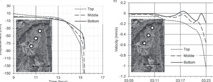
Based on the photogrammetric measurements [akca et al., 2011], increasing downslope movements

started about 2 hours before the failure in the mid-dle and upper parts of the slope (Fig. 14a). The ve-locity of movements at cluster 3 (top) is higher than in the middle and at the bottom. The movements start to accelerate about 30 minutes before the fail-ure and stepwise movements were measfail-ured during this period (Fig. 14b). These stepwise movements

Fig. 12 – The vertical component of displacements betwe-en the 28 and 31 October 2008 [akca et al., 2011].

Fig. 12 – Componente verticale degli spostamenti misurata tra il 28 e il 31 ottobre 2008 [akca et al., 2011].

occurred perhaps because ofthe pull out or break-age of the roots and/or the dilative behaviour of the soil mass in the shear band. As illustrated in figure 13 and discussed in 5.2, drops in the water content and piezometric level in the vicinity of the failure surface were recorded. These observations support a hypothesis of dilative behaviour of the soil or drain-age through tension cracks developing just prior to slope failure.

Some seconds before tension cracks appeared across the top of sprinkled area, the right side of the landslide followed the line along which the roots were cut (Fig. 15). It took about 36 seconds to mo-bilise about 130 m3 _{of debris. The water was} exfiltrat-ing from the back of the scarp after the failure (Fig. 15). The places where water oozed out from the bed-rock were mainly located on the upper right part of the slope. They can be indications of interconnected

Fig. 13 – a) Changes in the volumetric water content profile in cluster 3; b) Changes in the piezometric level at two points on the upper part of the slope (after askarinejad et al., 2010b).

Fig. 13 – a) Evoluzione del contenuto volumetrico di acqua nel cluster 3; b) Evoluzione della altezza piezometrica in due punti diversi nella parte alta del pendio (da aSkarinejad et al., 2010b).

Fig. 14 – a) The surface movements in the Z direction at three points on the failure wedge (time 0, is the start of the rain-fall); b) The changes in the velocity in the Z direction during 20 minutes before the failure (the coordinate system is shown in Fig. 20).

Fig. 14 – a) Movimenti superficiali in direzione Z in tre punti diversi nel cuneo di rottura (tempo 0, è l’inizio delle precipitazioni); b) Evoluzione della velocità in direzione Z durante i 20 minuti precedenti la rottura (il sistema di coordinate è mostrato in Fig. 20).

permeable layers, which transferred the water from the upper parts of the slope to these locations. This water flow applied an outward seepage force to the soil mass and functioned as a key triggering factor for the landslide.

6. Analytical limit equilibrium simulations

The equation for factor of safety has been de-rived for the infinite slope model, assuming a shal-low, translational soil movement along a planar sur-face parallel to the ground. In this equation, the shear strength of the soil is based on the effective stresses proposed by BishOp [1959] for unsaturated

soils.

s′ = (s – ua) + c(ua – uw) (8)

where s′ is the effective stress, s is total stress, ua

is pore air pressure, uw is pore water pressure, the

quantity s = (ua – uw)is matric suction, and c is a

ma-terial property that depends on the degree of satura-tion or matric sucsatura-tion.

In this section, it is assumed that:

c = Sr (9)

where Sr is the degree of saturation.

Bishop’s effective stress with, c = Sr will change to the saturated effective stress [Terzaghi, 1936] if the

pore pressures at the slip surface become positive. Nonetheless, the slip surface is presumed to be locat-ed above the water table where the soil is unsaturatlocat-ed. According to the assumptions mentioned above, the factor of safety (F.S.) for the 2D infinite slope (Fig. 16a) is determined by comparing the resisting shear force (Tf) along the slip surface with the

driv-ing force due to the weight (Wsina):

F.S. = Tf (10)

Wsina where W is the weight of the element

The force normal to the failure surface is: N = Wcos a = gh l 1cos2_{a (11)} The width of the element is assumed to be 1 m. F.S. = gh l cos2a tanj′ + Sr s tanj′ l + cr_b l ₍₁₂₎

gh l sin a cos a

F.S. = tanj′+ 2Sr s tanj′ + 2cr_b (13)

tana gh sin2a gh sin2a

where g is the unit weight of the soil in-situ, the cr_b

is the root reinforcement at the base of the element and b, h, a are geometric parameters defining the el-ement in the infinite slope (Fig. 16a).

The first term on the right hand side of the equa-tion (13) is the contribuequa-tion of fricequa-tion angle, the second term is the effect of apparent cohesion due to the unsaturated conditions, and third part is the contribution of the base root reinforcement.

The reinforcing effect of the roots in this section is conceptualised as resistant shear and normal tensile stresses, along the sides and base, and the upper face of the failure wedge, respectively. Estimates of the root reinforcement mobilised for the Ruedlingen slope are based on the distribution of the roots and the mechan-ical properties of the root bundles as a function of the displacement during pull out tests [SchWarz, 2011].

Perpendicular root models are used in con-ventional methods of root reinforcement quanti-fication [WaldrOn, 1977; Wu et al., 1979; Wu et al.,

1988; Wu and WaTsOn, 1998]. In these models, it is

assumed that the roots are located normal to shear zone and tension is transferred to them as the faces of the shear band are moving relative to each other. Confining stress increases due to the tensile force in the reinforcements [Bucher, 1983]. Another

impor-tant assumption of this method is that the full ten-sile strength of the roots is mobilised as the shear oc-curs (e.g. pOllen and simOn, 2005). However, field

and laboratory measurements of Ruedlingen case show that the maximum root bundle strength occurs

Fig. 15 – Shape of the failure wedge and locations of water outflow after the failure.

Fig. 15 – Forma del cuneo di rottura e punti di fuoriuscita dell’acqua dopo la rottura.

at larger strains than the typical strains at the maxi-mum soil strength.

This two dimensional limit equilibrium analysis (springman et al., 2003; casini et al., 2010b) is now

ex-tended to a three dimensional geometry with lateral-ly limited slides, in order to account for the resisting forces along the sides (Ts) of the failure wedge (Fig.

16b). The vertical and lateral reinforcing effect of the vegetation at the base and along the vertical planes of the failure wedge is estimated, respectively. The ef-fective depth of lateral root reinforcement (hr) can

be varied. Moreover, the effect of frictional resistance due to the horizontal soil pressures acting on the walls and the apparent cohesion are taken into account.

The factor of safety is again calculated by equa-tion (10):

F.S. = Tf = Tb + 2Ts (14) W sina W sina

where, Tb and Ts are the resisting forces mobilised

at the base and at the side of the block, respectively. The resisting force at the base (Tb) is:

Tb = Nb tanj′ + Sr s tanj′ BL + cr_bBL (15)

where B, L are the width and the length of the block respectively, (Fig. 16b), and Nb is the normal force to

the base plane:

Nb = Wcosa = g hBL cos2a (16)

where, g and h are the unit weight of the soil and the height of the wedge, respectively.

The resisting force at the sides of the wedge is: Ts = Ns tanj′ + Sr s tanj′ hL + cr_b hr L (17)

where cr_s is the root reinforcement at the sides of

the element, hr is the height of the root

reinforce-ment (Fig. 16b), and Ns is normal force applied to

the sides. For the sake of simplicity, a constant value of suction along the depth of the soil to the failure surface is assumed in this equation.

Ns = 1₂K g′ L h2 (18)

According to Equations (14) to (18) and assum-ing a horizontal pressure coefficient at rest (K0=1-sin

j′), the factor of safety will be:

F.S. =g h B L cos2a tanj′ + Sr s tan j′ B L + cr_bB L +

(19) gh B L cosa sina

+ 2(1/2 K0 gL h2 tanj′ + Sr s tanj′ h L cosa + cr_s hr L cosa)

gh B L cosa sina

F.S. =

Sr s tanj′

[

]

[

]

+ (20) cos2_{a B B cos}2_a gh tana + cr_b ₊ 2hr cr_s cos2_{a BLcosa} gh tana

The forces acting at the upper and lower ends of the block are ignored in this method, except for the root reinforcement, Tveg, which is evaluated in

sec-tion 7.3.

Parameters used for the soil, root reinforcement, and geometry in these analyses are listed in Table III.

Fig. 16 – a) The infinite slope model; b) The simplified three dimensional model.

Fig. 16 – a) Modello di pendio indefinito; b) Modello tridimensionale semplificato.

Tab. III – Parameters used for the infinite slope analyses.

Tab. III – Parametri usati nell’analisi di pendio indefinito. φ’ (°) γ (kN/m3₎ e α (°) h (m) L (m) b (m) cr_b (kPa) cr_s (kPa) hr (m) 32 16.33 1 38 1.1 17 7.5 0.5 4 0.3

The comparison between the 2 approaches based on equations (13) and (20), with different as-sumptions for the root reinforcement, is illustrated in figure 17. The factor of safety is calculated based on the wetting branch of the water retention curve for Ruedlingen soil, with e = 1.0 (Fig. 10).

The results show that the F.S. derived from the 2D approach for suctions lower than 4 kPa is 88% of the F.S. of 3D approach for the failure width of 7.5 m (on average).

The value for the reinforcing effect of the lateral roots is based on an extensive study of the pull-out and breakage forces of roots in the region. The se-lected value (cr_s = 4 kPa) is an average of the mea-sured maximal root reinforcement at the scarp of the failure zone. The measured values of the lateral root reinforcement vary between 0 to more than 10 kPa on this slope [schWarz, 2011].

The lateral root reinforcement is assumed to be uniformly effective at depths of 0 to 0.3 m in these analytical simulations. Comparing the chang-es in the F.S. shown in figure 17 for the 3D models, with and without lateral root reinforcement, it can be seen that the difference in the predicted F.S. is about 3%. This value shows the effect of cutting the roots along the longitudinal borders of the experi-ment site on the stability of this marginally stable slope.

6.2. Prediction of potential depth of failure surface The F.S. is set to 1.0, to establish the variation of minimum required suction (or degree of satura-tion) with the depth of the inclined failure plane, in order to predict the potential depth of failure and hence the volume of mobilised material [casini et al.,

2010b]. This is a key factor in landslide hazard as-sessment.

Equations (21) and (22) show the minimum ap-parent cohesion required to have a stable slope, in the 2 and 3 dimensional cases, respectively.

F.S. = 1 Þ c* =

[

]

[

(

)

]

[

]

The results are depicted in figure 18. The 2D in-finite slope methods, with different root reinforce-ment at the base, show an increasing value of re-quired apparent cohesion as the depth of failure in-creases. The 3D approach results in a critical depth of around 1.3 m as the suction decreases. This depth is similar in different scenarios of root reinforce-ment and agrees well with the average depth of fail-ure in reality (have = 1.1 m).

6.3. Effect of variability of root reinforcement with depth The vertical distribution of tree roots in the soil profile along the scarp is confined to the top 0.6 m of soil, whereas the root network of the grass plants was only effective in the first 0.2 m of soil, as reported by schWarz [2011]. The root network for both trees and

grass plants decays exponentially with depth, similar to the findings of previous researchers (e.g. aBe and

iWamOTO, 1990; schmidT et al., 2001; dOcker and huB -Ble, 2009). Accordingly, a conceptual model for the

lateral root reinforcement is considered with an ex-ponential decay in cohesion attributed to the roots from 0.15 m to 0.6 m in depth (Fig. 19a). The same

Fig. 17 – Comparison between 2D infinite slope and sim-plified 3D analysis, with and without vegetation.

Fig. 17 – Confronto tra le analisi di pendio indefinito 2D e 3D semplificata con e senza vegetazione.

Fig. 18 – Minimum required apparent cohesion for different failure depths (the arrows show the regions with F.S.>1).

Fig. 18 – Coesione apparente minima necessaria per diverse profondità di rottura (le frecce indicano la regione con F.S.>1).

approach will be applied, as in section 6.1, to calcu-late the factor of safety, with the difference of vari-able root effects and application of root reinforce-ment to the both side and back of the failure wedge (Tveg in Fig. 16b). No basal root reinforcement is

tak-en into account in this section.

Similar to equation (14), the F.S. can be written as:

F.S. = Tf = Tb + 2Ts + Tveg (23) W sina W sina

Tb is similar to equation (15) but without the term

accounting for the base root reinforcement.

Ts is the shear resistance on one side of the failure

wedge:

Ts = Ns tanj′ + Sr s tanj′ hL + Fveg_s (24)

where Ns is the normal force applied to the sides and

is calculated according to Equation (18), and Fveg_s is

the reinforcing force of the vegetation on one side of the failure wedge:

hr

Fveg_s = cos2a

∫

where clat is the value of root reinforcement,

accord-ing to Figure 19a.

Likewise, the reinforcing force provided by the vegetation at the back of the failure wedge (Tveg)

(Fig. 16b) is:

hr

Tveg =

∫

The factor of safety is compared for the first and the second experiments, after cutting the roots along the longitudinal borders of the field. Figure 19b, shows the changes in the F.S. with respect to the decrease in suction and the changes in the maxi-mum value of the root reinforcement. The effect of cutting the roots to the depth of 0.3 m along the lon-gitudinal bounds of the slope on the F.S. is consid-ered. clat_0 is the cohesion attributed to the roots at

the depth of 0 m of the soil. The difference in the F.S. between the first (full edge) and the second (cut edge) experiments is about 7% for the top root re-inforcement of clat_0 = 4 kPa. However, the factor of

safety is not lower than 1.0 within the positive range of matric suction (negative pore water pressure), if clat_0 > 3 kPa.

7. Two dimensional uncoupled numerical

simulations

The results of the uncoupled numerical simu-lations of the first and the second experiments are presented in this section. The simulations were per-formed using the SEEP/W and SLOPE/W modules of the GeoStudio software. The hydraulic boundary conditions were applied to the finite element mod-el produced with the SEEP/W and pore pressure distributions were calculated. The factor of safety

Fig. 19 – a) Conceptual model for decay of root reinforcement with depth; b) Parametric study on the stability effect of the maximum lateral root reinforcement.

Fig. 19 – a) Modello concettuale di decadimento del rinforzo delle radici con la profondità; b) Studio parametrico della stabilità dovuta al rinforzo laterale delle radici.

of the slope was determined using SLOPE/W and based on the pore pressure distributions exported from SEEP/W for each time step. The pore pres-sure distributions were calculated according to the Richards’ equation [richards, 1931] for pore fluid

flow in the unsaturated soil matrix. The laboratory results of water retention curve were fitted with the formula proposed by Van genuchTen [1980]. The

unsaturated hydraulic conductivity functions de-rived by Beck [2010] were calibrated and used in

the analysis.

The shear strength of the unsaturated soils was applied in SLOPE/W using Fredlund et al. [1978]

extended form of the Mohr-Coulomb criterion (Eq. 24).

t

= c

+ (s

– u

) tanj

+ (u

– u

) tan j

where jb _{describes the linear increase of the shear}

strength due to the increase of matric suction. This linear expression has been questioned in view of in-creasing experimental evidence [escariO and saez,

1986; Fredlund et al., 1987; alOnsO et al., 1990].

Un-fortunately, this cannot be considered by the GeoStu-dio software.

The relationship between j′ and jb _{can be}

de-rived by comparing equations 1 and 27. tanjb

= Sr = q (28)

tanj′ n

The most conservative value for jb _{is used in}

these simulations based on the residual volumetric water content and maximum insitu porosity.

The mechanical properties used for these simu-lations are summarised in table IV.

The reinforcement effect of the roots is imple-mented in the mechanical properties of the mod-el by introducing additional cohesion (cveg) to the upper 0.3 m of the top soil layer. The value is cho-sen based on the average measurements in the field [schWarz and rickli, 2008]. The calculation of the

factor of safety is performed based on the method of slices and with the approach of mOrgensTern and

price [1965], which considers the moment

equilibri-um of individual slices.

The geometry of the bedrock is derived from the DPL results. From the hydraulic point of view,

the bedrock is impermeable. It is also assumed to be mechanically stable under the simulated loads. It is modelled as an elastic material. The location and sizes of the fissures in the bedrock were deter-mined by monitoring the sequences of the changes in the degree of saturation in the soil and bedrock regions. The fissures were implemented in the geo-metry of the models and were filled with the over-lying soil, with similar hydro-mechanical properties. This assumption needs to be refined by further field investigations or by a parametric study of the hydrau-lic properties of the fissures and their effect on the drainage of the slope.

7.1. Simulation of the monitoring experiment (October 2008)

Figure 20 shows the geometry of the bedrock, lo-cation of the fissures, water flow paths and the satu-rated zone in the slope at the last time step before the rainfall stopped in the first Ruedlingen experi-ment. Infiltrating water flows towards and is drained by means of the fissures in the bedrock. Accordingly, it is assumed that these permeable fissures play a ma-jor role in stabilising the slope. The calculated factor of safety is lower than 1, for the critical slip surface of the first experiment but this simulation is a 2 dimen-sional one, and does not take into account the side friction mobilised at the lateral boundaries of the failure wedge. Therefore, the simulated pore pres-sures were used in a simplified 3 dimensional limit equilibrium model, as explained in section 6.1. As a result, the F.S. increased to 1.13, which implies sta-bility and is consistent with movements in the slope during the first experiment, but without developing failure.

Tab. IV – Mechanical properties adopted for the numeri-cal simulations.

Tab. IV – Proprietà meccaniche usate nelle simulazioni numeriche. g (kN/m3_{) (°)}j’ j b (°) (kN/mc’ 2_{) (kN/m}cveg 2₎ 16.3 32 10 0 4

Fig. 20 – Water flow paths and the saturated zone at the end of the rainfall [BischOF, 2010].

Fig. 20 – Percorsi del flusso d’acqua e zona di completa saturazione al termine dell’evento di pioggia [biSchOf, 2010].

7.2. Simulation of the triggering experiment (March 2009) 7.2.1. hYdraulicsimulaTiOns

The simulations were performed for the second experiment based on the geometry of the bedrock on the right hand side of the field (looking from the road) because the ERT measurements were per-formed on this side and also the failure occurred mainly on the right side of the slope. The ERT mea-surements and also field observations after the fail-ure indicate a fissfail-ure and a permeable horizontal in-trusion in the upper part of the bedrock (Fig. 20).

Since the rain intensity was not uniformly distrib-uted on the slope in the second experiment [askar -inejad et al., 2010b], seven zones were defined over

which different intensities were applied.

The infiltration simulations showed that the majority of the rain applied in the upper part of the slope was drained into the sub-vertical fissure and then through the horizontal intrusion to the slope body, applying an uplifting seepage force to the soil. This could be one of the main causes of triggering the failure. The inclination of the upper fissure was not clear either from the ERT measure-ments or from the field investigations. Therefore, a parametric study was performed on the effect of the inclination of this fissure. The results showed that a range of directions of fissures provide dif-ferent time spans for the water to reach the inter-face between the bedrock and the soil through the permeable horizontal intrusion. Hence, the incli-nation can delay the exfiltration of water from the bedrock.

The suction changes were monitored in the up-per part of the model corresponding to the location

of cluster 3 (C.3 in Fig. 5) on the slope. One of the monitoring points on the model was on the surface, and the other one was at the interface between the soil and the bedrock, at a depth of 1.2 m. Figure 21 shows the comparison between the simulated suc-tions from the numerical model and the measured suction in-situ. The curves follow similar trends. The increase of suction at the surface due to ceasing ap-plication of rain can be seen in the data obtained from the numerical solution.

The difference of 2 to 3 kPa between the mea-sured and simulated values of suction could have several causes, such as the uncertainties and simpli-fications in the model, the precision of the measure-ments, and the difference in the initial conditions of pore water pressure between the model and the slope in reality.

Fig. 21 – Comparison between the simulated suction chan-ges to the in-situ measured values (after BischOF, 2010).

Fig. 21 – Confronto tra suzione misurata e ottenuta dalle simulazioni numeriche (da biSchOf, 2010).

Fig. 22 – a) The geometry of the bedrock on the right hand side of the slope and location of the critical slip surface; b) En-larged section showing the critical slip surface and the saturated zone (dashed curve) [BischOF, 2010].

Fig. 22 – a) Geometria del substrato roccioso a destra del pendio e posizione della superficie critica; b) Sezione ingrandita della superficie di scorrimento critica e zona di completa saturazione (zona tratteggiata), [biSchOf, 2010].

7.2.2. FacTOrOFsaFeTY

No reinforcing effects of the roots were tak-en into account in these simulations, because the roots along the sides of the slope were severed to the depths of 0.3 to 0.4 m before the experiment, although this is only relevant for the right hand boundary of the failure zone (Fig. 5).

The critical slip surface based on the method of slices, (which is quite similar to the real slip surface) has a factor of safety equal to 0.76, after 15 hours of rainfall. After performing the corrections for the 3 dimensional effects, and without root reinforce-ment, F.S. = 0.83.

The critical slip surface is shown in figure 22. 7.3. Root reinforcement effect in the second experiment

Analyses have been conducted with root rein-forcement over the upper 0.3 m of the soil layer. The comparisons are shown in figure 23. The factor of safety increases with a magnitude of 0.1 during the experiment, after introducing the root effects. The minimum value of F.S. is reached 3 hours after the rainfall stops.

8. Summary and conclusions

Field and laboratory investigations have provid-ed a comprehensive set of data both to characterise the ground and to record the hydro-mechanical re-sponses of a silty sand slope during artificial rainfall events. The hydrological characterisations revealed a bottom to top saturation pattern [springman et al.,

2012] for the soil profile in the study area, and also the possibility of drainage into the bedrock.

A comprehensive laboratory characterisation has been performed on natural and statically

com-pacted samples of Ruedlingen soils. Since the aver-age slope of the field exceeds the critical state in-ternal friction angle, the partial saturation and the reinforcement of the root and possibly the shape of the bedrock combine to play a fundamental role in stabilising the slope.

The instantaneous profile method was used to derive the hydraulic conductivity function of the soil in unsaturated conditions. The results [Beck, 2010]

show a decrease of two orders of magnitude in the conductivity with increasing suction to 40 kPa.

The spatial distributions of reinforcing effects of the roots were studied. The reinforcement was quantified and used in the analytical and numeri-cal simulations. However, the estimated values for the root reinforcement along the scarp of the failure were higher than the values that were back calculat-ed from the limit equilibrium method. Apart from the simplifications made in the models, one reason for this difference can be that the fine roots have a strong seasonality; hence there are less superficial fine roots in winter (when the landslide occurred) than in summer (when the calibration was done) [schWarz, 2011].

Photogrammetry was successfully used to moni-tor the surface movements during the slope mon-itoring and landslide triggering experiments and helped to identify the area of the slope most at risk prior to failure. This has important implication for early warning systems and counters the assumption that such failures are abrupt and lack early clues and limited possibility of forecasting [campBell

1975].

The mechanical features of unsaturated soils and reinforcing effects of the vegetation were im-plemented in simple infinite slope limit equilibrium analysis and results were compared to the analyti-cal three dimensional limit equilibrium simulations. The three dimensional geometries included laterally limited slides of the failure wedge. Basal and lateral root reinforcements have been introduced in these models. The results show reasonable values for the factor of safety, despite the simplifications in these models.

Based on these simplified 3-D models, the possi-ble depth of the failure surface was calculated at 1.1 m (Fig. 18) for a factor of safety of 1. The calculat-ed values agrecalculat-ed quite well, with the in-situ measure-ments at 0.8 to 1.3 m.

As confirmed by the 2D uncoupled hydro-me-chanical finite element simulations, the hydraulic in-teraction of the bedrock with the overlying soil lay-ers, in terms of drainage and exfiltration, can play a major role in the pattern of pore pressure distri-butions and in stabilising or destabilising the slopes. A more complex 3D finite element analysis is being performed at present in order to take the coupled response of soils into account.

Fig. 23 – Comparison of the changes in F.S. for the slope with or without root reinforcement [BischOF, 2010].

Fig. 23 – Confronto dell’evoluzione del fattore di sicurezza per il pendio con e senza il contributo delle radici [biSchOf, 2010].