1
Autore:
Dr. Ing. Marco Brogioni Firma__________
Relatori:
Dr. Ing. Paolo Pampaloni Firma__________
Modeling microwave emission from
snow covered soil
Anno 2008
UNIVERSITÀ DI PISA
Scuola di Dottorato in Ingegneria “Leonardo da Vinci”
Corso di Dottorato di Ricerca in
Telerilevamento
“Labor improbus
omnia vincit”
3
ACKNOWLEDGMENTS
This work has been carried out in the frame of the research projects of the Microwave Remote Sensing Group of the Institute of Applied Physics (IFAC)- Italian National Research Council.
First of all, I want to thank Dr. Ing. Paolo Pampaloni, my tutor and pioneer of the microwave remote sensing in Italy, for introducing and leading me into this beautiful branch of scientific research. His lectures, advice, discussions and, above all, his rigorous ethics have been fundamental for my studies. Before I met him I barely knew what microwave remote sensing was, and now I am grateful to him for the discovery of this “new world”.
I would also like to thank Dr. Ing. Giovanni Macelloni, my officemate, Dr. Simonetta Paloscia, Dr. Ing. Emanuele Santi, Dr. Ing. Simone Pettinato, Mr. Roberto Ruisi and Dr. Pietro Poggi for their significant help and collaboration in my research and their friendship.
Part of my work in developing the IRIDE model was carried out at the Institute for Computational Earth System Science (ICESS) of the University of California-Santa Barbara under the supervision of Prof. Jiancheng Shi. I am very grateful to him for having hosted me at UCSB and spent his precious time discussing about electromagnetic models for natural surfaces.
Last, but not least, I must thank my family for supporting me during these harsh times, when the work of the people is considered only a hateful cost and the young researchers seem to be children who don’t want to grow up and stop playing.
I
SOMMARIO
Il ciclo idrologico rappresenta l’insieme di tutti i fenomeni legati alla circolazione e alla conservazione dell’acqua sulla Terra. Il monitoraggio su scala globale dei fattori che concorrono a produrre e modificare tale ciclo (umidità del terreno, copertura vegetale, estensione e caratteristiche del manto nevoso) risulta di estrema importanza per lo studio del clima e dei cambiamenti globali. Inoltre, l’osservazione sistematica di queste grandezze è importante per prevedere condizioni di rischio da alluvioni, frane e valanghe come pure fare stime delle risorse idriche. In questo contesto Il telerilevamento da satellite gioca un ruolo fondamentale per le sue caratteristiche di osservazioni continuative di tutto globo terrestre. I sensori a microonde permettono poi di effettuare misure indipendentemente dall’illuminazione solare e anche in condizioni meteorologiche avverse. I processi idrologici, ed in particolare quelli della criosfera (la porzione di superficie terrestre in cui l’acqua è presente in forma solida), sono fra quelli che meglio si possono investigare analizzando la radiazione elettromagnetica emessa o diffusa. Mediante l’utilizzo di modelli elettromagnetici che permettono di simulare l’emissione e lo scattering da superfici naturali è possibile interpretare le misure elettromagnetiche ed effettuare l’estrazione di quelle grandezze che caratterizzano i suoli e la loro copertura.
In questo lavoro di dottorato si è affrontato il problema della modellistica a microonde dei terreni coperti da neve, sia asciutta che umida. Dopo aver preso in considerazione i modelli analitici maggiormente utilizzati per simulare diffusione ed emissione a microonde dei suoli nudi e coperti da neve si è proceduto allo sviluppo e implementazione di due modelli di emissività. Il primo, basato sulla teoria delle fluttuazioni forti, è atto a descrivere il comportamento di un manto nevoso umido. Il secondo, basato sull’accoppiamento del modello di scattering superficiale AIEM (Advanced Integral Equation Method) con la teoria del trasferimento radiativo nei mezzi densi, è volto allo studio di uno strato di neve asciutta sovrastante un suolo rugoso. Tali modelli tengono conto degli effetti coerenti presenti nell’emissione del manto nevoso e non inclusi nella teoria del trasporto radiativo classico. Entrambi i codici sono stati validati con datasets numerici e sperimentali in parte derivati da archivi ed in parte ottenuti nel contesto di questo lavoro che ha previsto quindi anche una fase sperimentale. Quest’ultima è stata condotta con misure radiometriche multifrequenza su un’area di test situata sulle Alpi orientali. Le simulazioni ottenute con questi modelli e le conseguenti analisi hanno permesso di individuare la sensibilità della temperatura di brillanza ai parametri di interesse (spessore, equivalente in acqua e umidità del manto nevoso) in funzione di diverse configurazioni osservative (frequenza, polarizzazione ed angolo di incidenza). Questo ha consentito di migliorare la comprensione dei meccanismi di emissione dalle superfici innevate e di individuare le migliori condizioni osservative per un sistema di telerilevamento terrestre.
III
ABSTRACT
The hydrologic cycle represents the whole of the phenomena related to the circulation and preservation of the water on the Earth. The global scale monitoring of the factors involved in the production and modification of such cycle (e.g. soil moisture, vegetation cover, snow cover characteristics and extent) is extremely important for climatologic and global changes studies. Moreover, the systematic observation of such factors is important to forecast the risk of floods, landslides and avalanches as well as to estimate the water resources. In this context satellite remote sensing plays a fundamental role for its characteristic of systematic and continuous observation of the entire Earth’s surface. Besides, microwave sensors allow performing measurements independently of solar illumination and weather conditions. The hydrological processes, especially the ones in the cryosphere (the part of Earth’s surface in which the water is in solid form), are the ones which can be better investigated by analyzing the electromagnetic radiation emitted or scattered by natural surfaces. By using electromagnetic models, which simulate emission and scattering from natural surfaces it is possible to interpret the electromagnetic measurements and to perform the retrieval of the parameters that characterize the soil and its covers.
This thesis deals with the microwave modeling problem of soils covered by snow (both dry and wet). After a detailed review of the most used analytical models for simulating scattering and emission from soil (both bare and covered by snow), two emissivity models have been developed and implemented. The first one, based on the Strong Fluctuation Theory, is devoted to describe the wet snowpacks behavior. The second one, based on the Advanced Integral Equation Method surface scattering model coupled with the Dense Media Radiative Transfer Theory, is devoted to study a layer of dry snow overlying a rough soil. Both of these models account for the coherent effects that take place in the emission of snowpacks and which are not accounted for by the conventional radiative transfer theory. The two snow software have been validated against numerical and experimental datasets derived from archives and from experimental measurements carried out during this thesis work. This latter activity has been worked out by means of multifrequency radiometric measurements taken on a test area on the Eastern Italian Alps. The simulations performed by means of the two models allowed us to determine the sensitivity of the brightness temperature to the most interesting geophysical parameters (thickness, water equivalent and wetness of snow) as a function of different observation configurations (frequency, polarization and incidence angle). Such work made it possible to significantly improve the knowledge of the emission processes of snow covered areas and to determine the best observation configuration for an Earth remote sensing system.
V
Index
1. INTRODUCTION ... 1
2. STATE OF THE ART... 5
2.1 Scattering and emission from soils ... 8
2.1.1 The dielectric constant of bare soils ... 8
2.1.2 Characterization of soil roughness ... 10
2.1.2.1 Statistical description ... 10
2.1.2.2 Fractal description... 11
2.1.3 The electromagnetic models for bare soil ... 12
2.1.3.1 The Small Perturbation Method (SPM) ... 13
2.1.3.2 The Kirchhoff approach ... 14
2.1.3.3 The Small Slope Approximation ... 17
2.1.3.4 The IEM model and its evolutions (IEMM and AIEM) ... 19
2.2 Scattering and emission from a snow layer ... 28
2.2.1 The Strong Fluctuation Theory ... 28
2.2.1.1 Wave approach ... 30
2.2.2 Dense Medium Radiative Transfer Theory (DMRT) ... 32
2.2.2.1 Approximation of multiple scattering equations (Quasi-Crystalline Approximation, QCA, and QCA with Coherent Potential, QCA-CP)... 37
2.2.2.2 Effects of size distribution... 40
2.2.3 Frequency behavior of snow models ... 42
3. MODELING THE EMISSION FROM SNOW COVERED SOIL ... 45
3.1 Bistatic scattering from soil: the Advanced Integral
Equation Method (AIEM) ... 46
3.1.1 The model ... 46
3.1.2 The reflection coefficients ... 54
3.1.3 The shadowing effects... 56
3.1.4 The autocorrelation functions... 56
3.1.5 Polarimetric version of the AIEM ... 57
3.1.6 Validation of the AIEM ... 61
3.1.6.1 Gaussian ACF L-band ... 62
3.1.6.2 Gaussian ACF C-band... 62
3.1.6.3 Exponential ACF L-band ... 64
VI
3.1.7 Comparison between AIEM simulations and experimental
data ... 67
3.1.7.1 Gaussian ACF : Smooth surface... 69
3.1.7.2 Gaussian ACF : “Rough” surface ... 71
3.1.7.3 “Medium rough” mixed ACF surface... 71
3.2 Electromagnetic properties of a dry snowpack: the Dense
Media Radiative Transfer model (DMRT) ... 72
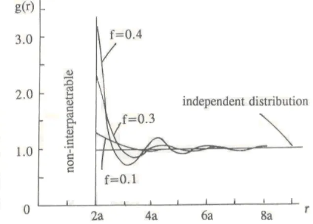
3.2.1 The pair distribution function for sticky particles... 73
3.2.2 The effective permittivity and the extinction coefficient ... 75
3.2.3 The DMRT-QCA phase matrix ... 79
3.3 Emission from a dry snow layer upon a rough soil ... 83
3.3.4 Computation of the reflection coefficients ... 92
3.4 Modeling snow containing free liquid water (wet snow) ... 93
4. EXPERIMENTAL RESULTS AND COMPARISON WITH SIMULATIONS ... 97
4.1 Comparison of the snow emission model with
experimental data ... 97
4.1.1 The IFAC remote sensing equipment and experiments ... 97
4.1.2 The Morsex (Microwave and Optical Remote Sensing experiment) dataset ... 98
4.1.2.1 Comparison between the snow model and the Morsex dataset of dry snow... 100
4.2 The effect of the liquid water on the emission of snow... 104
5. SENSITIVITY ANALYSIS OF THE DMRT MODEL ... 109
CONCLUSIONS ... 117
BIBLIOGRAPHY ... 117
Appendix 1: Validation of the AIEM model ... 129
Exponential correlated surfaces ... 129
Gaussian correlated surfaces ... 162
Appendix 2: The permittivity of a dense medium computed by
the SFT... 169
List of symbols
Re[..] and Im[..] real and imaginary part of a complex number
J, i imaginary unit
A scalar quantities
A
,A
vectorsA
,A
matrices“×” and “⋅” vector and scalar products ∇×[..], ∇⋅[..] rotor and divergence operators <…> ensemble average operator
x0, y0, z0 unit vectors for Cartesian coordinates
r0, θ0, φ0 unit vectors for polar coordinates
E(r,t) electric field vector in the time domain [Volt/m] H(r,t) magnetic field vector in the time domain
E(r) electric field vector in the frequency domain (ω is tacit) or electric field phasor H(r) magnetic field vector in the frequency domain (ω is tacit) or magnetic field phasor
G Dyadic Green’s function
Ex, Ey, Ez cartesian components of the electric field
Er, Eθ, Eφ polar components of the electric field
Eh, Ev horizontal and vertical components of the electric field (E h=Eφ; Ev=Eθ)
ρ, ρm electric and magnetic charge volumetric densities (charge densities)
K effective propagation constant
Ei and Es incident and scattered field in a scattering problem
K=β-jα electromagnetic wave vector
kx, ky, kz cartesian coordinates of the wave vector
e-jk⋅r ejωt space and time dependence of a plane wave phasor (sign rule for Fourier transforming in the time and space
domains)
F Frequency or Fractional volume of ice crystals in snow
λ wavelength
K=2π/λ wavenumber
C speed of light in vacuum
ε0, µ0, k0 dielectric constant, magnetic constant and wavenumber of vacuum
εc=ε’-jε” complex dielectric constant of the medium (including conductive losses)
εr=εr’-jεr” relative dielectric constant of the medium
VIII
εb air permittivity
εs permittivity of ice crystals
εg auxiliary permittivity (in SFT)
ξi susceptibility
g(r) pair distribution function
η characteristic impedance of the medium Pr Power flux density at receiving point [Watt/m2]
Pt power flux density from transmitting antenna [Watt/m2]
Pi incident power flux density (on the target) [Watt/m2]
Ps or wR scattered power flux density (from the target) [Watt/m2]
A, w, t absorbance, surface albedo and transmittance of a layer or a semi-infinite medium
ke extinction rate
e and eλ emissivity and spectral emissivity
W, ϖ surface albedo or single scattering albedo (depending on the context)
Bλ or Bf spectral radiance/brilliance [Watt/ster/m
2/µm or
Watt/ster/m2/Hz]
TB brightness temperature [K]
I incident direction unit vector (corresponding to direction in polar coordinates θ
i, ϕi)
S observation (scattered) direction unit vector (corresponding to direction in polar coordinates θ
s, ϕs)
R distance between two points (i.e., observation point wrt source points) R distance of a point from origin of coordinate system σ(θi, ϕi; θs, ϕs;
pi,ps)= σ(i, s; pi,ps)
bistatic radar cross section for incidence direction θi, ϕi,
polarization of incident wave pi, observation direction θs, ϕs
and observed polarization ps.
σ°(θi, ϕi; θs, ϕs;
pi,ps)= σ°(i, s;
pi,ps)
bistatic scattering coefficient for incidence direction θi, ϕi,
polarization of incident wave pi, observation direction θs, ϕs
and observed polarization ps. (as defined in Ulaby et al.,
1986) γ(θi, ϕi; θs, ϕs;
pi,ps)= γ(i, s; pi,ps)
As above, but following the definition by [Tsang et al., 2000].
f(I, s) scattering amplitude, being Es(r)= f(i, s) e-jkr/r
σa, σs, σe absorption, scattering and extinction sections [m2]
ξs, ξa scattering and absorption efficiencies
ka, ks, ke absorption, scattering and extinction volumetric coefficients [m-1]
τ(r1, r2) and t(r1,
r2)=e-τ
optical depth and path transmittance from range r1 to range
r2
Rh(θ) and Rv(θ) Fresnel reflection coefficients for H and V polarization and incidence angle θ, respectively
and incidence angle θ, respectively T Stickiness of ice particles
) , , , (θφθ′φ′ P phase matrix ) ( 10 θ T transmissivity matrix
ΓH(θ), ΓV(θ) plane surface specular reflectivity for H and V polarization, respectively
θB Brewster angle (or pseudo Brewster angle)
ζ(x,y) height of a rough surface above the mean plane (random function of coordinates x,y) lx correlation length of a random function x (subscript can be omitted)
µx and µx mean value of random variable x or of a random vector x, respectively
σx and σx2 standard deviation and variance of a random variable x (or random function)
ρx(∆t)=ρx(τ) and ρ x(∆r)
autocorrelation function of a stationary random function x (of time t or space r)
ρxy: correlation coefficient between two random variables x and y
S=∂y/∂x sensitivity of radiative quantity y (measured by the sensor) to geophysical quantity x. mv, mg volumetric and gravimetric soil moisture, respectively
SMC soil moisture content (either mv or mg)
1
1. INTRODUCTION
In the recent years there has been a growing interest in the weather global changes and in the management of the natural resources. The attention paid by the media to the climate increases every day and raises the alertness of the common people to the environment care. Moreover, people have been further scared by natural disasters like the hurricane Katrina, the Indian Ocean tsunami and floods in central Europe. The demand of knowledge about “what is happening to our planet” and “how these changes could be avoided” pushes the researchers to deeply investigate the natural phenomena and understand how to minimize the impact of the humankind on the environment.
At the same time, the reasons to improve our knowledge about the Earth are also driven by other factors. Besides the noble spirit of understanding our planet, there are economic and politic motivations. For example, the possibility of predicting the precipitation rate during the crop growth seasons can influence the life of large areas of the world by adopting appropriate countermeasures against the famine and by the speculation of the economic lobbies. In addition, the knowledge of some hydrological variables such as soil moisture, vegetation cover and the quantity of snow deposed during the winter season on the mountains is important for the agriculture, to evaluate the risk of floods and avalanches and also to drive the energy choices of the electrical companies.
In this scenario, the understanding of the Earth dynamics is very important and the remote sensing (RS) can play a fundamental role due to its intrinsic characteristics, e.g. the possibility to investigate remote and inaccessible areas and perform analysis very often (on daily or weekly basis). The remote sensing is based on the analysis of the electromagnetic (e.m.) radiation scattered or emitted by the natural bodies. Depending on the characteristics of the e.m. waves measured it is possible to deduct some features of the observed objects. The possibility to understand the state of an object being far from it let the remote sensing very attractive.
There are several areas in which the RS can be applied successfully. Among the majors: weather forecasts, land classification, and study of the processes involved in the hydrological cycle. This latter topic is considered very important because it represent the basis to understand the climate and its changes.
The hydrological cycle (see Fig. 1) is made up by several components. The main ones are: precipitations (rainfall, snowfall and hail), soil moisture, accumulation of snow and ice, water run-off and evaporation. Among them, one which can be investigated using at most the characteristics of remote sensing is the cryosphere (the portions of the Earth's surface where water is in a solid form). Indeed, the areas with snow covers are very often inaccessible and dangerous but they need to be accurately monitored. For instance, let us considering Antarctica which contains more than 95% of the fresh water on Earth and which influences the world climate due to its high albedo. Monitoring the Antarctic environment is very difficult using classical techniques. In fact the mean annual temperature is far below -30°C letting Antarctica be one of the most impervious place where the man can
live and operate. Thus, the use of satellite remote sensing techniques can result very useful.
Fig. 1 - The hydrological cycle
Snow cover has the largest area extent of any component of the cryosphere and, except Antarctica, most of the Earth’s snow-covered area is located in the Northern Hemisphere, where the mean snow-cover extent ranges from 46.5 million km2 in January to 3.8 million km2 in August [1]. The temporal variability is dominated by
the seasonal cycle. However, changes in the annual spatial distribution of snow have been observed during the last decades related to the global warming [2]. The terrestrial cryosphere plays a significant role in the global climate, in climate response to global changes and as an indicator of change in the climate system. Moreover, remote sensing of the melting cycle of snow has proven to be crucial to forecast the snow-water runoffs, floods and avalanches, besides to manage water resources.
The remote sensing techniques are based on sensors that operate in different portions of the electromagnetic spectrum. For land applications, the researchers commonly use the optical part (which ranges from the far infrared to the ultraviolet) or the microwaves (electromagnetic waves with a frequency that span from 300 MHz to 300 GHz). The interaction of the e.m. waves with the natural bodies happens in two different ways which are strictly related one to the other. When the radiation impinges on a body, it can be both absorbed and scattered away (depending on the geometrical and physical properties the object). According to the Plank’s law, in thermodynamic equilibrium the energy absorbed equals the one re-emitted. The two phenomena, absorption/emission and scattering are bound together by the principle of energy conservation. Microwave sensors can be either passive or active and can both operate on entire frequency spectrum. Passive sensors (radiometers) measure scattered radiation emitted by the sun in the optical range, or thermal emission emitted by the Earth’s surface in the infrared and
3 microwave bands. Active sensors (lidar and radar) measure scattered radiation emitted by their own illuminating sources.
Remote sensing of snow has traditionally been carried out mostly by using optical sensors [3]. Several operational services have been established to obtain snow cover maps from the NOAA AVHRR sensors. These sensors have a poor resolution (1 km), but provide a reasonable temporal coverage (daily products) depending on cloud conditions. Indeed this is the biggest limitation to the use of optical instruments. The electromagnetic waves in the visible and infrared spectra cannot penetrate the clouds that let the optical sensors blind. Conversely, microwave sensors are almost insensitive to the weather phenomena. In general, there is an optimum sensor configuration (frequency range, polarization and incidence angle) for each observed target. For instance, the best frequency band to estimate soil moisture has been identified at L-band. Conversely, the observation of dry snow requires the use of higher frequencies that, at present are available in passive sensors only. Indeed, several experiments have documented the ability of C-band Synthetic Aperture Radar for mapping the extent of wet snow only by using both ERS and RADARSAT data [4]-[6]. Automated algorithms are available using change detection. However, due to its high transparency at C-band, dry snow cannot be separated from bare soil.
The sensitivity of microwave emission to snow type and water equivalent (SWE) has been pointed out in several theoretical [7]-[12] and experimental [13]-[22] studies which demonstrated the potential of microwave radiometers in monitoring snow parameters and seasonal variations in snow cover. Unfortunately, the rough spatial resolution of satellite sensors from satellite, such as the Special Sensor Microwave Imager (SSM/I), limited their effectiveness in operational use. The improved performance of the Advancing Microwave Scanning Radiometer (AMSR-E) on the Earth Observing (EOS) AQUA platform helps to partially overcome this drawback [23].
Radiation emitted at the lower frequencies of the microwave band (lower than about 10 GHz), by soil covered with a shallow layer of dry snow is mostly influenced by the soil conditions below the snow pack and by snow layering. At higher frequencies, however, the role played by volume scattering increases, and microwave emission becomes sensitive to snow cover [14],[15]. In general, high frequency microwave emission from dry snow decreases as snow depth (SD) increases, although SSM/I measurements taken within the former Soviet Union during the 1987–1988 winter period showed significant deviations from this pattern [21]. If snow melts, the presence of liquid water in the surface layer causes an increase in emission. The average spectra of the brightness temperature show that emission of dry and refrozen snow decreases with frequency, whereas emission from wet snow displays an opposite trend. Experiments carried out in the Swiss Alps by Hofer and Mätzler [15], by using ground-based sensors demonstrated that microwave radiometers can separate three snow conditions (winter, spring and summer) representative of the seasonal development of snow cover. These trends were interpreted by Schanda et al. [16], who pointed out the dominant role played by the Rayleigh scattering, and confirmed by other experiments (e.g. [18]). Further
4
investigations pointed out the importance of the snow crust, which can build up due to the night-time refreezing [24], [25].
The most important snow quantities to be monitored for applications are: extent of snow cover, snow liquid water content, and snow water equivalent. Regarding the liquid water content of snow (LWC) several retrieval algorithms have been developed. For instance, in [26] an algorithm based on polarimetric C-band SAR data is shown. Fully polarimetric information is needed to separate the effects of surface roughness from the effects of LWC. Since Envisat-ASAR only has dual polarization it has not been possible to study LWC solely from SAR. However, a combination of SAR and in situ measurements from synoptic weather measurements in Finland has revealed promising results.
The determination of the beginning of the snow melting is crucial in flood forecast and avalanche prevention. The potential of microwave radiometers in measuring snow wetness has been pointed out in [22]. Snow water equivalent (SWE) is the most important and highest valued snow parameter from a hydrological point of view. It is computed by the product between snow density and snow depth. Usually the SWE is defined for dry snowpack and it indicates the whole amount of water that will run-off to the valley during the spring season. As stated above, the retrieval of SWE from C-band SAR backscattering is very problematic, although some interesting result has been obtained over relatively smooth surfaces in cold regions [27]. A new approach to retrieve information on the changes in SWE from repeat pass interferometric phase changes was introduced by Guneriussen et al. [6] and tested in a drainage area in Norway. The method invokes advanced delta-k processes to avoid phase wrapping. Data were calibrated with corner reflectors not covered by snow.
To analyze experimental measurements and understand the interaction between electromagnetic waves and targets, models which describe the emission and scattering must be used. Depending on the degree of approximations of physical laws and on the method to calculate some parameters it is possible to obtain several kind of models which span from the empirical (the simplest but the less accurate to describe the observed medium) to the physical ones which are based on the electromagnetic theory and are the most complex.
To describe the electromagnetic emission or scattering from snow-covered surface, two models must be used: one for the soil and one for the snow. These models will be described in the following section.
This work is organized as follows: a comprehensive review of the state of the art for scattering and emission models for bare soil and snow is given in section two. Section three includes the description of the models developed to simulate the electromagnetic emission from Alpine snowpack, pointing out the improvements obtained in this work and the critical points. A comparison of model simulations with experimental data is outlined in section four.
2. STATE OF THE ART
A crucial problem of remote sensing is the retrieval of geophysical parameters from the measured electromagnetic radiation. This is an inversion problem that requires the use of appropriate direct models. In the last decades several models and techniques have been developed to analyze and simulate the interaction between microwaves and snow-covered surfaces. Depending on the approach followed to describe the electromagnetic behavior of the snowpack or to retrieve physical parameters, the models used to predict microwave emission and scattering can be divided in the following three groups: empirical, semi-empirical and theoretical. The choice of the method is closely related to the final application.
The empirical models are based on experimental relationships between remote sensing and ground data, and make use of regressions (or other kind of statistical analysis) to estimate soil and snow parameters [28]-[32]. The important matter is to have a large dataset of both electromagnetic measurements (or simulated data) and snow and soil physical parameters.
For instance in [33] the SD is estimated by
(
T
HT
H)
SD
=
1
.
59
18−
37 (1)Where and are respectively the 18 GHz and 37 GHz horizontally polarized brightness temperatures, and 1.59 is a constant obtained by a linear regression of the difference between 18GHz and 37GHz responses. If the 18GHz brightness temperature is less than the 37GHz one, no snow is assumed present.
H
T
18T
37HThe limits of these algorithms are the area over which they can give good predictions and the errors on the estimations which are relatively high. Considering that the electromagnetic emission depends simultaneously on several parameters of the snowpack but also on the ground features and on the vegetation coverage, it is easy to understand why the estimations can be different if they are made on the north European tundra or on the Asian desert.
Anyway, these algorithms are useful when the estimations are made on a global scale (tents or hundreds of squared kilometers). In this case, it is very difficult to have spatially detailed description of the surface, which, on the other hand, may include different types of coverage in the coarse spatial resolution elements of the spaceborne instruments. Thus, the use of methods that leave out detailed knowledge of the observed surfaces is very attractive and sometimes mandatory.
5 The procedure to develop an empirical algorithm is quite simple. The only need is two big datasets of conventional and electromagnetic measurements which will be split in two parts: the first half is used to establish the relationship and the other one to test the performance of the algorithm. Then, by using regressions (whether linear, quadratic, exponential, etc.) or artificial neural networks (ANN) relationships between the two kinds of data can be found and verified. It is possible to estimate snow physical parameters from electromagnetic measurements or also to predict the scattering and emission from conventional ones.
As stated before, the performances of these algorithms are not very good both because the study area are seldom homogeneous (and the electromagnetic signal of the snow is influenced by the one of the vegetation and other sources), and because the microwave emission/scattering strongly depends on several parameters (the retrieval of the geophysical parameters from the e.m. measurements is an ill-posed problem). Sometimes it is simpler to retrieve global parameters like the Snow Water Equivalent (which is defined as the integral of the snow density along the vertical profile of the snowpack) instead of snow depth and density separately. Anyway, in some cases the empirical algorithms have excellent performance. For instance, the retrieval of the snow temperature profile in Antarctica from AMSR-E radiometric measurements: the retrieval error has resulted to be lesser or equal than 1°C [31] because the structure of the snowpack remains almost unchanged year after year.
The semi-empirical models are based on physical laws (hence are more rigorous than the empirical ones) but, for the determination of some parameters they use experimental data. An example is the HUT (Helsinki University of Technology) model [34] which has been successfully used to simulate the microwave brightness temperature of a simplified snowpack configuration.
The approach used in the HUT snow emission model to estimate the brightness temperature of snow-covered soil relies on the following assumptions: the scattered microwave radiation is mostly concentrated in the forward direction and the snowpack is a single homogeneous layer overlying a semi-infinite half space (the ground). Thus, the brightness temperature inside a snowpack of depth d, just below the snow–air boundary, can be approximated as follows [34]:
(
)
↑ − − − − + −−
≡
+
−
+
=
Bg Bs d k q k s e snow a d k q k b be
T
T
k
q
k
T
k
e
T
d
T
e s e s , , sec ) ( sec ) (1
)
,
0
(
)
,
(
θ
θ
θ θ (2)where θ is the observation angle, is the soil brightness temperature just above the ground–snow interface, is the snowpack physical temperature, q is an empirical parameter ( q = 0.96 ) describing the fraction of intensity scattered in the direction θ which is the same at all frequencies, and k
)
,
0
(
+θ
bT
snowT
e, ks, and ka are,respectively, the extinction, scattering and absorption coefficients (ke =ks+ ka). It is
easy to recognize in (2) that the first term of the right hand side is the ground contribution attenuated by the overlying layer while the second represents the contribution from the snow. The extinction properties of dry snow (i.e. ke in (2)) as a
function of snow grain size are modeled like in [35]. ka is calculated from the
complex dielectric constant of dry snow. The real part of the snow dielectric constant is determined by using the formulas given in [36] whereas the imaginary part is treated with a formula based on the Polder–Van Santen mixing model [37]. To calculate the imaginary part of snow permittivity, the ice dielectric properties are also required. These are computed using an empirical formula [36]. The effect of snow grain size is described through the extinction coefficient, as determined empirically in [35]
2 8 . 2
0018
.
0
f
φ
k
e=
(3)where is in decibels, f is the frequency in gigahertz, and φ is the snow grain diameter in millimeters. Equation (3) was derived from observations on natural snowpack characterized by grain diameters ranging from 0.2 to1.6 mm.
e
k
Another example of semi-empirical model is the Microwave Emission Model of Layered Snowpacks (MEMSL) valid in the frequency range 5-100 GHz that has been developed by Wiesman and Mätzler [11] for dry winter snow and extended to wet snow by Mätzler and Wiesmann [12]. This model is based on multiple scattering radiative transfer theory, in which the scattering coefficient is determined from measurements of snow samples.
The theoretical models are, among the three categories, the most rigorous and are based on the solution of the Maxwell’s equations. These models need an accurate characterization of the media interacting with the electromagnetic waves and are more useful to understand the phenomena which happen rather than estimate the physical properties of the target by inverting the experimental data. Indeed, the formulae describing the scattering or the emission are usually non-linear and very complex. Moreover the electromagnetic problem is multiparametric and ill-posed (different combination of input parameters give the same e.m. prediction), making almost impossible to invert the equations (theoretical methods).
The most used theoretical models for simulating surface scattering from soil are the Small Perturbation Method (SPM), the Kirchhoff Approach under the Physical and Geometrical Optics approximations (respectively KA-PO and KA-GO), the Integral Equation Method (IEM) and the Small Slope Approximation (SSA). For volume scattering from the snowpack the most advanced models are based on the Strong Fluctuation Theory (SFT) and the Dense Medium Radiative Transfer Theory (DMRT). All of these models have been successfully used within their limits of validity to simulate emission and scattering. A comprehensive description of these models is given in the following chapter.
Among the said models, the most used for the soil is the IEM, which has a wider validity domain than the SPM and the KA. In snow applications, the SFT and the DMRT use different approaches to model the snowpack (continuous for the SFT and discrete for the DMRT) but the results are similar; although, in recent years the DMRT has been improved and now, seems to reproduce experimental data better than the SFT over a wider range of frequencies.
The main problem with the theoretical models is the difficulty to solve exactly the Maxwell equations in the case of media with a complex structure such as the natural bodies. Usually several approximations can be made (see [38] for snow) leading to more or less wide validity ranges. Another issue, which is strictly bound to the complexity of the models, is the computational time. Until few years ago the computational power of the computers was quite lower than what it is now and this
8
led the researcher to obtain simpler models. In the recent times, these problems are less severe and it is possible to use more complicated methods.
It is worth noting also that with the advent of modern computers and the development of fast numerical methods, numerical simulations of the wave scattering problems have become an attractive alternative overcoming the limitations in regimes of validity of classical analytical models. An excellent treatment of various approaches can be found in the book by Tsang et al. [39]. A good review of the numerical methods is given also in the introduction of the paper by Li et al. [40].
2.1 Scattering and emission from soils
The electromagnetic scattering of the bare soils is usually modeled like surface scattering. This kind of scattering happens at the interface between two media that are homogeneous but with different electromagnetic properties. The former hypothesis is verified for the air but not exactly for the terrain, which is actually heterogeneous. Anyway, by considering the high density of the scatterers and the relatively high permittivity of its components, it is possible to compute an effective dielectric constant for the soil and to re-conduct the whole scattering problem to the classical surface one.
The problem of the scattering from a bare soil can be divided into three different sub-problems, which need to be solved:
- first of all, the soil can be modeled like a mixture of lime, clay, sand and water. Thus the effective permittivity of such mixture must be calculated on the basis of the percentage and the dielectric constant of each element. - second, the roughness statistic of the interface must be determined
through the shape of the autocorrelation function (ACF), and the related Height Standard Deviation (HStdD), (known also as Standard Deviation of Soil heights, SDS), and the correlation length. A different approach is the determination of the fractal features of the surface.
- finally, depending on the previous parameters, the electromagnetic problem must be solved by using appropriate approximations.
2.1.1 The dielectric constant of bare soils
Natural terrains can be regarded as mixtures of bulk material (sand, clay, loam, silt organic material, etc) and water, bounded by a rough surface. The determination of the electric properties of a mixture (the “homogenizations” problem) has been investigated since the nineteenth century [41]. Conversely, from the homogeneous media, the heterogeneous ones have electrical properties which depend on several factors: e.g. the percentage of the components, their permittivity and permeability, and the chemical bond between the molecules. A comprehensive description of the methods developed to obtain the effective dielectric constant of a mixture can be found in [41]. Usually mixing formulas that average the permittivity of each constituent by means of their percentage are used. However, when the differences between the electrical properties of the components are sensible, the models
become more complicated. This is the case of soils, in which the permittivity of dry material (usually close to 3) is much smaller than that of water.
The dielectric characteristics of water have been investigated in several textbooks and papers (e.g. [42]). The complex permittivity ε of pure free water can be described by the Debye equation:
τ π ε ε f j n n s 2 1 2 2 + − + = (4)
where n is the refractive index, εs is the static dielectric constant, f is the frequency,
and τ is the relaxation time. On the other hand, the permittivity of soil is also dependent on soil texture since the particle dimensions of soil components vary from less than 2 µm for clay to more than 1000 µm for sand. Thus, for the same volumetric moisture content, there is more free water in sand than in clay.
One of the most used models to calculate the dielectric constant of the terrain is semi-empirical and has been developed by Dobson et al. [43]. It assumes the soil made up by a four-component mixture and the resulting permittivity can be expressed as α α α α α
ε
ε
ε
ε
ε
soil=
v
ss ss+
v
a a+
v
fw fw+
v
bw bw (5)where the subscripts ss, a, fw, bw stand for solid soil, air, free water and bounded water and
0
7
.
4
j
ss≅
−
αε
φv
v
ss= 1
−
v av
m
v
=
φ−
(6) bw fw vv
v
m
=
+
b ss b ssv
ρ
ρ
ρ
ρ
φ≅
1
−
0
.
38
−
=
In (6)
v
φ is the soil porosity,ρ
ss≅
2.65 gr/cm3 is the density of the soil solidmaterial and is the total volumetric moisture content. To simplify the model but still retain a soil textural dependence it is possible to group together the water parameters as v
m
α β α αε
ε
ε
fw bw bw v fw fwv
m
v
+
≅
(7)where β is a parameter empirically determined. Using (7) the soil permittivity can be written as
(
1
)
(
1
)
1
+
−
+
−
≅
α β α αε
ε
ρ
ρ
ε
ss v fw ss b soilm
(8) 9Dobson et al. [43] determined empirically the remained parameters α and β. They found that the value α=0.65 was the best compromise for all the soil types, whereas the magnitude of β can vary from 1.0 for sandy soil to 1.17 for silty clay. Generally, β can be estimated by
C
S
0
.
18
11
.
0
09
.
1
−
+
=
β
(9)where S and C are respectively the weight fraction of the sand and the clay in the soil.
2.1.2 Characterization of soil roughness
2.1.2.1 Statistical description
A rough surface can be described by a height function z = f(x,y). Direct assessment of roughness can be carried out by means of various experimental approaches able to reproduce the surface profile by using contact or laser probes. However, the exact characterization of natural surfaces is, in general, very difficult. The problem of defining optimal parameters for natural surface roughness has been investigated in many studies (e.g. [44]-[49]). In general, the analysis of scattering in remote sensing is performed by using random rough surface models, where the elevation of surface, with respect to the mean plane, is assumed to be a stationary stochastic process with a Gaussian height distribution. A different method of surface characterization is based on fractal description of surfaces [44].
An isotropically rough surface can be described by a one-dimensional random function z = f (ρ,φ) with zero mean, i.e. <f (ρ,φ)> = 0. For a stationary random process, we have:
)
(
)
,
(
)
,
(
2 1 2 2 2 1 1φ
ρ
φ
σ
ρ
ρ
ρ
f
=
C
−
f
z (10)where σz is the height standard deviation and C is the autocorrelation function
(ACF) which is a measure of the correlation of surface profile f(ρ) at two different locations ρ 1 and ρ 2.
The most common ACFs used in remote sensing of land surfaces are the Gaussian correlation function
) exp( ) ( 2 2 l C
ρ
= −ρ
(11)and the Exponential correlation function:
) exp( ) ( l C
ρ
= −ρ
(12)where l is the correlation length. The spectral densities are respectively:
(
2 2)
2 1 ) ( l k l k W z ρ ρ =π σ+ (13) 10for the exponential ACF and ⎟ ⎟ ⎠ ⎞ ⎜ ⎜ ⎝ ⎛ − = 4 exp 2 ) ( 2 2 2l k l k W z ρ ρ σ π (14)
for the Gaussian one.
Besides these two functions, several other kinds of autocorrelation functions have been developed and applied. It is worth quoting the mixed-exponential and the 1.5-power which behave like an exponential for smooth surfaces and like a Gaussian for rough ones. In [50] several power ACF have been analyzed, pointing out that this type of functions shows the best performance in modeling the roughness of natural soils with respect to the Gaussian and exponential ones.
In addition to the height function f(ρ), the slope function α(ρ) = f’(ρ) (<α(ρ)> = 0) is also an important characterization of the rough surface. Given a stochastic process, its derivative is also a stochastic function. If a random surface f (ρ) is generated by a Gaussian process its derivative f’(ρ) is also Gaussian and its slope variance s2 is related to the second derivative of its correlation at the origin i.e. [51]:
) 0 ( " 2 2 2 2 2 C l s z σz σ =− = (15)
For the exponential correlation function the rms slope does not exist. This implies that this kind of ACF does not work for very rough surfaces. On the other hand, several measurements on natural surfaces have shown that the exponential ACF best represents the soil roughness. These two facts are contradictory: some explanations could be that ground measurements are not much accurate (maybe due to the finite length of the instruments) or that more complex ACF types must be considered in the modeling. In [52] a multi-scale approach has been analyzed: the exponential-like correlation function was simulated by the sum of three X-power ACFs, which are differentiable and have physical insight. The results show that a possible reason of the exponential correlation of most natural surfaces is that they contain more than one scale of roughness and that a multi-scale ACF can represents better the natural roughness of soil.
2.1.2.2 Fractal description
An interesting alternative approach is to model the surface by a continuous fractal function [53]. This technique can provide a new description of natural soils, since fractals are suitable tools for describing mixtures of deterministic and random processes. A fractal analysis of perfectly conducting bi-dimensional profiles has been performed by Rouvier and Borderies [54], who pointed out the fractal nature of the scattered field. The characterization of soil roughness and backscattering in terms of fractal Brownian description has been studied by Zribi et al. [55], who also validated a model using experimental data. On the other hand, several scientists (e.g. [56]-[58]) have shown that the slope and intercept of the power spectrum of the soil profile can be additional significant descriptors of the topography of natural soils. Moreover, slope S of the power spectrum, computed in a log-log space, makes it possible to determine the fractal parameter D according to the relation: D = (5 + S)/2 [59].
Differently from the common descriptors of roughness (σx and l), the fractal
dimension is a parameter which describes the scaling properties of a surface, i.e. it possesses the property of self similarity. The fractal dimension can be estimated by using the classical method of box counting or from the power spectrum of the surface profile.
A basic problem involves incorporating these roughness descriptions into existing scattering models to provide essentially the same information as the traditional parameters.
2.1.3 The electromagnetic models for bare soil
The most common analytical models of scattering by dielectric rough surfaces are the Small Perturbation Method (SPM) and the Kirchhoff Approach (KA) under both the Physical and Geometrical Optics solutions (respectively PO and GO). An updated comprehensive treatment of these two approaches is given in [51] and in [39]. Further advances include the small slope approximation (SSA) [60]-[63] and the Integral Equation Method [64],[65]. The starting point for all of these approaches is the Huygens principle, which expresses the field at an observation point in terms of fields at the boundary surface (e.g. [51]). The scattered intensities are usually decomposed into coherent and incoherent terms.
The limits of validity of these approaches have been frequently discussed in literature, but an exact criterion has not yet been exactly established. Anyway the plot in Fig. 2 show the commonly accepted validity range of SPM, PO, GO and IEM in the ks-kl plane [66]. kL PO SP GO AIEM 0.1 1 10 0.1 1 10 100 ks M kL PO SP GO AIEM 0.1 1 10 0.1 1 10 100 ks 0.1 1 10 0.1 1 10 100 ks M
Fig. 2 - The validity range of the SPM, PO, GO and AIEM
From Fig. 2 it can be easily seen that the validity range of the AIEM cover both the SPM and the KA approximations letting it one of the most versatile models for the surface scattering.
2.1.3.1 The Small Perturbation Method (SPM)
The SPM, which is valid when the surface variations are much smaller than the electromagnetic wavelength and the slopes of the rough surface are relatively small, has found extensive applications in active and passive remote sensing of land surfaces. In this model, the random surface z = f(x,y) is decomposed into its Fourier spectral components. The scattered wave consists of a spectrum of plane waves. The scattered fields can be solved by using the Extended Boundary Condition method with the perturbation method. In the EBC method the surface currents are calculated first by applying the extinction theorem. The scattered fields can then be calculated from the diffraction integral by making use of the calculated surface fields [51]. The solution for the one dimensional surface is given in [51]. The more complete analysis, carried out up to the second order solution of the three dimensional problem with two-dimensional dielectric rough surfaces assures energy conservation and can be found in [39]. In this approach the zero order solution consists of only a single spectral component, which is simply the Fresnel specular reflection from a flat surface at z = 0.
In the first order solution the incoherent bistatic scattering coefficient for a Gaussian correlation function assumes the form [67]:
(
)
4 2 2 2 2 4 0 2 2cos
cos
4
,
,
,
l k qp i s i i s s qp de
f
l
k
ρθ
θ
σ
ϕ
θ
ϕ
θ
σ
=
ς − (16)where θs, φs θi, φi are the incident and azimuth scattered and incident angles,
[
sin2 sin2 2sin sin cos( )]
2 2 i s i s i s d k
kρ= θ + θ − θ θ φ −φ , and the fqp terms are given in [67] as functions of the wave-numbers in free space and in the medium, the z components of incident and transmitted propagation vectors, and the incident and scattering angles.
The first order solution does not modify the coherent reflection coefficients and, to see the correction term for the coherent wave due to the rough surface, the second order solution must be calculated. In the second order solution, the bistatic scattering coefficients as given in [39] are the following:
[
⊥ ⊥ ⊥ ⊥ ⊥ ⊥ ⊥ ⊥]
⊥ ∞ ∞ − ⊥ ⊥ ⊥ ⊥ ⊥ ⊥ ⊥ ′ + ′ − + ′ ⋅ ⋅ ′ − ′ ′ − = = − °∫
k d k k k k k f k k k f k k k f k k W k k W k i i ee i ee i ee i s i i s s hh ) , , ( , , ( ) , , ( ) ( ) ( cos 4 ) , ; , ( * * 2 2 ) ) )θ
π
φ
θ
π
ϕ
θ
σ
(17)[
⊥ ⊥ ⊥ ⊥ ⊥ ⊥ ⊥ ⊥]
⊥ ∞ ∞ − ⊥ ⊥ ⊥ ⊥ ⊥ ⊥ ⊥ ′ + ′ − + ′ ⋅ ⋅ ′ − ′ ′ − = = − °∫
k d k k k k k f k k k f k k k f k k W k k W k i i he i he i he i s i i s s vh ) , , ( , , ( ) , , ( ) ( ) ( cos 4 ) , ; , ( * * 2 2 ) ) )θ
π
φ
θ
π
ϕ
θ
σ
(18) 13[
⊥ ⊥ ⊥ ⊥ ⊥ ⊥ ⊥ ⊥]
⊥ ∞ ∞ − ⊥ ⊥ ⊥ ⊥ ⊥ ⊥ ⊥ ′ + ′ − + ′ ⋅ ⋅ ′ − ′ ′ − = = − °∫
k d k k k k k f k k k f k k k f k k W k k W k i i hh i hh i hh i s i i s s vv ) , , ( , , ( ) , , ( ) ( ) ( cos 4 ) , ; , ( * * 2 2 ) ) )θ
π
φ
θ
π
ϕ
θ
σ
(19)[
⊥ ⊥ ⊥ ⊥ ⊥ ⊥ ⊥ ⊥]
⊥ ∞ ∞ − ⊥ ⊥ ⊥ ⊥ ⊥ ⊥ ⊥ ′ + ′ − + ′ ⋅ ⋅ ′ − ′ ′ − = = − °∫
k d k k k k k f k k k f k k k f k k W k k W k i i eh i eh i eh i s i i s s hv ) , , ( , , ( ) , , ( ) ( ) ( cos 4 ) , ; , ( * * 2 2 ) ) )θ
π
φ
θ
π
ϕ
θ
σ
(20) where:o
k
⊥,
k
i⊥,
k
⊥′
, are wave vectors denoting scattering, incident and intermediatedirections respectively
o W(k⊥− k⊥′) is the spectral density of the rough surface The functions fee, fhe, fhh, feh are given in [39].
2.1.3.2 The Kirchhoff approach
Physical Optics (PO)
The Kirchhoff approximation, which is valid when the radius of curvature at every point on the surface is much larger than the wavelength, assumes that the fields at any point on the surface are equal to the fields that would be present on an infinite tangent plane at that point. Even with this approximation, no analytic solution has been obtained for the scattered field without further simplifications. The expression of the scattered field contains the integral of a function F(α, β) where α and β are the local slopes of the surface f(x,y). In one case (physical optics PO), for surfaces with small height standard deviation σ, the integrand function F(α, β) is expanded about zero slope and only the first terms F(0,0) are kept.
The bistatic scattering coefficients can be decomposed into a coherent and an incoherent part. For a large illuminated area, the bistatic scattering coefficient for the coherent component, which only exists in the specular directions, is:
)
(
)
(
)
cos
4
exp(
4
2 2 2 2 0 i s qp i s qp i po Cqpπ
R
k
σ
θ
δ
θ
θ
δ
φ
φ
σ
=
−
ς−
−
(21) where:o subscript p represent polarization of the incident wave and subscript q the polarization of the scattered wave
o Rpo is the reflection coefficient (b is for vertical or horizontal polarization)
o δqpis the Kronecker delta
The bistatic scattering coefficient for the incoherent component is given by equation [67]:
e
m!
m
)
k
(
e
l
|
)
,
(
q
|
)
4
k
(
=
m /(4m) l ) k + k ( 2m dz k -2 2 p s 2 qp 2 2 dy 2 dx 2 dz 2 F∑
∞ =⋅
°
1(
)
σ
β
α
σ
σ (22) where:o qs = hs or vs (horizontal or vertical directions of the scattered field)
o k = 2π/λ = wave number o λ = electromagnetic wavelength
o α , β = local slopes along x and y directions
o θi, φi, θs, φs = incident and scattering incident and azimuth angles
o Rh, Rv = Fresnel reflection coefficients
o l = surface correlation length o σ = height standard deviation o Fq(α,β )= f ( α,β,Rh,Rv,θi,θs,φs,φi ) o
k
dx=
k
⋅
(
sin
θ
i⋅
cos
φ
i−
sin
θ
s⋅
cos
φ
s)
o
k
dy=
k
⋅
(
sin
θ
i⋅
sin
φ
i−
sin
θ
s⋅
sin
φ
s)
o kdz=k⋅(cosθi+cosθs)
Geometrical Optics (GO)
When the wavelength is much smaller than the surface height standard deviation, we can assume under the geometrical optics limit (GO) that scattering occurs only along directions for which there are specular points on the surface excluding local diffraction effects. The bistatic scattering coefficients are proportional to the probability of the occurrence of the slopes, which specularly reflect the incident wave into the observation directions. The asymptotic solutions to the vector scattering integrals can be obtained using the stationary-phase method. In this approach the coherent component vanishes and the cross-polarized backscattering coefficient is zero since the Fresnel coefficients are evaluated at normal incidence. The bistatic scattering coefficient is expressed by [39]:
ab dz dy dx dz s i d qp
f
C
k
k
k
C
k
k
k
k
⎥
⎥
⎦
⎤
⎢
⎢
⎣
⎡
+
−
×
=
°
)
0
(
"
2
exp
)
0
(
"
2
ˆ
ˆ
2 2 2 2 2 4 4 4 ς ςσ
σ
σ
(23) where: o fqp = g (kx, ky, kz, ksx, ksy, ksz, σ, Rh, Rv, θi, θs, φi, φs)o (kx, ky, kz) and (ksx, ksy, ksz) = components of incidence (ki) and scattered (ks)
wave vectors
o kd = ki- ks = {kdx, kdy, kdz}
o C”(0) = second derivative of the autocorrelation function computed in the origin
It should be noted that the bistatic scattering coefficients satisfy reciprocity but violate energy conservation i.e. by ignoring multiple scattering there is a loss of energy.
Moreover, at high incidence angle the shadowing effect, which is neglected in the previous formula, becomes important. To take this effect into account the bistatic coefficients can be modified by introducing a shadowing function derived by Smith [68] and Sancer [69] (see also [39]). The modified coefficients σm
qp become:
( )
s i qp( ) ( )
s i s i m qpk
ˆ
,
k
ˆ
σ
k
ˆ
,
k
ˆ
S
k
ˆ
,
k
ˆ
σ
=
(24) where:( )
( )
( )
( )
( )
⎪
⎪
⎪
⎩
⎪
⎪
⎪
⎨
⎧
Λ
+
Λ
+
≥
+
=
Λ
+
≥
+
=
Λ
+
=
otherwise
k
k
S
i s s i i s i i s i s s s sµ
µ
ϑ
θ
π
φ
φ
µ
ϑ
θ
π
φ
φ
µ
1
1
,
1
1
,
1
1
ˆ
,
ˆ
(25)( )
⎥ ⎥ ⎦ ⎤ ⎢ ⎢ ⎣ ⎡ ⎟⎟ ⎠ ⎞ ⎜⎜ ⎝ ⎛ − = Λ − s erfc e s s 2 2 2 1 2 2 2 µ µ π µ µ (26)( )
l
h
C
s
=
σ
ς"
0
=
2
(27)In (25) and (26) µ=cot(θ). By adding this factor, the energy budget is improved, but the sum of reflected and transmitted energy is always less than unity and the difference is higher for H polarization [39].
An analytical theory for polarimetric scattering by 2D dimensional anisotropic Gaussian surface based on second order Kirchhoff approximation has been developed in [70]. The study was developed for any surface slope and height distributions assumed to be statistically even. The model is based on the geometric optics and takes into account the shadowing effect within the first- and second-order illumination functions. The computation of the incoherent scattering coefficient requires only threefold integrations allowing a relatively small computer time. It has been shown that the cross incoherent scattering coefficient is nil due to the shadow. The second-order incoherent scattering coefficient is proportional to the product of two surface slope probabilities for which the slopes would specularly reflect the rays in the double scattering process. In addition, the slope distributions are related to each other by a propagating term, equal to the modified characteristic function derived over the elevation difference where both reflections occur. This result generalizes the one obtained by Sancer [69] for any process in the case of single scattering.
Simulations performed with various versions of the model (first and second order), with and without shadowing were compared with numerical simulations in [71]. From the obtained results, a general conclusion of the applicability of the method 16

![Fig. 6 – Structure of the simple snowpack modeled like in [92]: there is one layer of snow above a semi-infinite medium (the soil)](https://thumb-eu.123doks.com/thumbv2/123dokorg/7307392.87915/46.723.125.619.441.690/fig-structure-simple-snowpack-modeled-layer-infinite-medium.webp)