ON HYBRID CENSORED INVERSE LOMAX DISTRIBUTION:
APPLICATION TO THE SURVIVAL DATA
Abhimanyu Singh Yadav1
Assistant Professor, Department of Statistics, PUC, Mizoram University, Aizawl-796001 Sanjay Kumar Singh
Professor, Department of Statistics and DST-CIMS, Banaras Hindu University, Varanasi-221005
Umesh Singh
Professor, Department of Statistics and DST-CIMS, Banaras Hindu University, Varanasi-221005
1. Introduction
In survival analysis, the study of the lifetime of any random phenomenon is an extensive work to explain the characteristics of existing phenomenon. Several life time models namely exponential, gamma, Weibull, etc. are introduced in market to illustrate the real pattern of failure data in medical as well as in engineering sciences. The generalized version of these models are also advocated and well jus-tified for the different situations of the failure rate behavior, see Ebrahimi (1990). The Lomax distribution is one of these and frequently used in economics, geogra-phy, econometrics and medical fields, see; Chandrasekar et al. (2002), Kleiber and Kotz (2003), Kleiber (2004).
The considered distribution belongs to inverted family of distributions and found to be very flexible to analyze the situation where the non-monotonicity of the failure rate has been realized, see Singh et al. (2012). If a random variable Y has Lomax distribution, then X = 1
Y has an Inverse Lomax distribution (ILD).
It has been used to obtain the Lorenz ordering relationship among ordered statis-tics; Kleiber (2004). Besides this, it has also lots of applications in stochastic modeling, economics and actuarial sciences, see Kleiber and Kotz (2003). Kleiber (2004) have implemented this model on geophysical data, particularly on the sizes of land fires in California state of US. Rahman et al. (2013) have discussed the es-timation and prediction problems for the inverse Lomax distribution via Bayesian approach. Yadav et al. (2016) have used this distribution for reliability estimation based on Type-II censored observations. But no one has paid attention about
the consideration of hybrid censored observation from ILD in both classical and Bayesian approach. Therefore, the authors have considered this problem under in-vestigation. The probability density function and cumulative distribution function of ILD are given by the following equations.
f (x, α, β) = αβ x2 ( 1 + β x )−(1+α) ; x≥ 0, α, β > 0 (1) where, α is the shape parameter and β is the scale parameter of the distribution.
F (x) = ( 1 +β x )−α ; x≥ 0, α, β > 0 (2) respectively.
The reliability and hazard functions, denoted as R(t) and H(t) of the ILD for specified values of t are given in following equations,
R(t) = 1− ( 1 + β t )−α ; t > 0 (3) and H(t) = αβ(1 + β t)−(1+α) t2(1− (1 +β t)−α ) ; t > 0 (4)
In industrial Statistics, censored observations are preferred due to cost, time or some other constraints. Hence, the variety of censoring schemes are used to ob-tain the censored observations. In practice most commonly used censoring schemes are Type-I and Type-II censoring schemes. In any life time experiments, exper-imenters are unable to investigate each experimental units. Therefore, generally experiments are terminated at prefixed time T or after getting predetermined number of failure R. In Type-I censoring scheme the termination time T is fixed and number of failure R is random and vice versa for Type-II censoring scheme respectively.
Hybrid censoring scheme is the mixture of Type-I and Type-II censoring schemes and it can be described as follows; Suppose n identical units are put on test and test is terminated when a pre-chosen number R out of n items are failed, or when a prefixed time T on the test has been obtained. Such censoring scheme is called as hybrid censoring scheme and it was introduced by Epstein (1954). This cen-soring scheme is quite useful in reliability acceptance plan, see MIL-STD-781-C (1977). Many authors have used this censoring scheme for their different purpose; see Draper and Guttman (1987), Chen and Bhattacharya (1988), Ebrahimi (1990) and the references cited therein. Hybrid censoring scheme is also comprises in two parts due to specification of censoring parameters R and T . In Type-I hybrid censoring scheme; suppose n units put on test, then experiment is terminated at the random time T∗ = M in(XR:n, T ), where R and T are prefixed numbers
and xR:n is the time of Rth failure in a sample of size n. Type-I hybrid
censor-ing scheme has its own limitations as conventional Type-I censorcensor-ing. The main demerits of Type-I hybrid censoring scheme, the number of observed failures is
at least one and there may be very few failures at the termination time of the experiment. Thus, it has the adverse effect over the efficiency of the estimators. Therefore, Childs et al. (2003) introduced a new type of censoring scheme which is an alternative to the Type-I hybrid censoring scheme, called as Type-II hybrid censoring scheme. In this censoring scheme, we terminate the experiments at the random time T∗ = M ax(XR:n, T ). The advantage of this scheme is that at least
R failures are observed at the end of the experiment. Fairbanks et al. (1982) have
obtained the exact distribution of the maximum likelihood estimator (MLE) of the mean and interval estimates in one-parameter exponential distribution based on a hybrid type II censored data. Banerjee and Kundu (2008) considered the statistical inference of the two-parameter Weibull distribution based on Type-II hybrid censored samples. Several works are available in the literature, see for ref-erences Gupta and Kundu (1998), Kundu and Pradhan (2009), Dube et al. (2011) etc.
The organization of the paper is as follows; In Section 1, we described the problem and hybrid censoring scheme. The maximum likelihood estimation is discussed in Section 2. Bayesian estimation procedure is carried out in Section 3. The numerical illustration of the considered methodology for the ILD are provided by considering two data set in Section 4. Finally, the conclusion of the paper is given in Section 5.
2. Maximum Likelihood Estimation
Case 1: Under type-I hybrid censored data (HCD-I)
In this section, we assume that the data are Type-I hybrid censored, then we have the one of the following types observations;
Data(X) =
{
x1:n< x2:n<· · · < xr:n when xr:n≤ T
x1:n< x2:n<· · · < xd:n when xr:n> T
(5) where, d denotes the number of failure observed before time T . Thus, the likeli-hood function for given p.d.f (1) under Type-I HCD is written as;
L(α, β|x) = n! (n− r)!α rβr [ 1− ( 1 + β xr:n )α](n−r) ∏r i=1 x−2i ( 1 + β xi )−(1+α) when xr:n≤ T n! (n− d)!α dβd [ 1− ( 1 + β xd:n )α](n−d) ∏d i=1 x−2i ( 1 + β xi )−(1+α) when xr:n> T (6) therefore, the combined likelihood function is given as;
L(α, β|x) = n! (n− m)!α mβm [ 1− ( 1 + β R )α](n−m) m∏ i=1 x−2i ( 1 + β xi )−(1+α) (7)
where; m = { r when xr:n≤ T d when xr:n> T (8) and R = { xr:n when xr:n≤ T xd:n when xr:n> T (9) Hence, the log-likelihood function is written as;
L = ln L(α, β|x) = Const. + m ln α + m ln β− 2 m ∑ i=1 ln xi− (1 + α) m ∑ i=1 ln ( 1 + β xi ) + (n− m) ln [ 1− ( 1 + β R )α] (10)
now for MLE’s of the parameters, we differentiate the log-likelihood function w.r.t to the parameter and equate to zero. Then, we have two likelihood equations which are obtained in implicit form. Therefore, N-R method is used to secure MLE’s. Hence, ∂L ∂α = m α − m ∑ i=1 ln ( 1 + β xi ) − (n− m) ( 1 + β R )α 1− ( 1 + β R )α ln ( 1 + β R ) = 0 (11) and ∂L ∂β = m β − m ∑ i=1 1 + α xi+ β − (n− m)α ( 1 + β R )α−1 R [ 1− ( 1 + β R )α] = 0 (12)
Let ˆα and ˆβ are the MLE’s of the parameters, then the MLE’s of the reliability
and hazard functions are given by using the invariance properties of MLE, which are obtained as;
ˆ R(t) = 1− ( 1 + ˆ β t )−ˆα and H(t) =ˆ α ˆˆβ(1 + ˆ β t)−(1+ˆ α) t2[1− (1 + βˆ t)−ˆα ]
The exact distribution of the maximum likelihood estimators are not available, thus, we derived the 95% asymptotic confidence interval based on fisher informa-tion matrix. The Fisher informainforma-tion matrix can be obtained by using equainforma-tion (10). Thus we have I( ˆα, ˆλ) = −∂2L ∂α2 − ∂2L ∂α∂β − ∂2L ∂β∂α − ∂2L ∂β2 ( ˆα, ˆβ)
where, the derivatives are given as, ∂2L ∂α2 =− m α2 + (n− m) ( 1 + β R )α[ ln ( 1 + β R )]2 [ 1− ( 1 + β R )α] 1 + ( 1 + β R )α [ 1− ( 1 + β R )α] ∂2L ∂α∂β = ∂2L ∂β∂α=− m ∑ i=1 1 (xi+ β) + (n− m)α ( 1 +β R )α−1 R [ 1− ( 1 +β R )α] 1 + ln ( 1 + β R )α + ( 1 +β R )α ln ( 1 +β R )α [ 1− ( 1 +β R )α]2 (13) ∂2L ∂β2 =− m β2 + m ∑ i=1 1 + α (xi+ β)2 + (n− m)α ( 1 + β R )α−2 R2 [ 1− ( 1 + β R )α] (α− 1) − α ( 1 + β R )α [ 1− α ( 1 + β R )α]
All the derivatives are evaluated at the point ( ˆα, ˆβ). The above matrix can be
inverted to obtain the estimate of the asymptotic variance-covariance matrix of the MLEs and diagonal elements of I−1( ˆα, ˆβ) provides asymptotic variance of α
and β respectively. Then by using large sample theory a two sided 100(1− δ)% approximate confidence interval for α and β are constructed as;
[ ˆαL, ˆαU] = ˆα∓ Zδ/2 √ var( ˆα), [ ˆβL, ˆβU] = ˆβ∓ Zδ/2 √ var( ˆβ) respectively.
Case 2: Under Type-II hybrid censored data (HCD-II)
If the data is Type-II hybrid censored, then we have one of the following types observations; Data(X) = x1:n< x2:n<· · · < xr:nwhen xr:n≥ T x1:n< x2:n<· · · < xd:n when xr:n< T x1:n< x2:n<· · · < xn:n complete data (14)
likelihood function under Type-II HCD is given as; L(α, β|x) = n! (n− r)!α rβr [ 1− ( 1 + β xr:n )α](n−r) ∏r i=1 x−2i ( 1 + β xi )−(1+α) when xr:n≥ T n! (n− d)!α dβd [ 1− ( 1 + β xd:n )α](n−d) ∏d i=1 x−2i ( 1 + β xi )−(1+α) when xr:n< T αnβn n ∏ i=1 x−2i ( 1 + β xi )−(1+α) whenCompletedataobserved (15) therefore, the combined likelihood function is given as;
L(α, β|x) = n! (n− m∗)!α m∗βm∗ [ 1− ( 1 + β R )α](n−m∗) m∏∗ i=1 x−2i ( 1 + β xi )−(1+α) (16) where; m∗= r when xr:n≥ T d when xr:n< T n when xr:n<· · · < xd:n< T (17)
All the other mathematical expressions can be obtained by replacing m by m∗ in the expression of HCD-I.
3. Bayesian Estimation
In this section, we considered Bayes procedure to obtain the point and interval estimates of the parameters α, β in presence of hybrid censored data. The Bayes estimators are derived under Jeffrey’s non-informative priors with squared error loss function. The considered priors are improper but they leads the proper pos-terior. Thus, the joint prior is given as;
π1(α, β)∝ 1
αβ ; α, β > 0 (18)
Then by using (7), (16) and (18) the joint posterior under considered cases (HCD-I, HCD-II) are given by;
p(α, β|x) ∝ αmβm [ 1− ( 1 + β R )α](n−m) ∏m i=1 xi ( 1 + β xi )−(1+α) αm∗βm∗ [ 1− ( 1 + β R )α](n−m∗) m∏∗ i=1 xi ( 1 + β xi )−(1+α) (19)
Now, after simplification the Bayes estimators of α, β, reliability function R(t) and Hazard function H(t) under SELF are simply obtained by taking the mean of the posterior distribution. From above, we noticed that the posterior distributions are not in explicit form. Therefore, it seems to be tedious to calculate the pos-terior expectations analytically. Therefore, Markov Chain Monte Carlo (MCMC) method has implemented for obtaining the approximate solution of the posterior expectations.
3.1. Markov Chain Monte Carlo Method
Here, we used Metropolis Hastings algorithm to extract the sample from poste-rior distribution to obtain the approximate Bayes estimates of the parameters and reliability characteristics. Further, we have also constructed 95% highest poste-rior density (HPD) credible intervals of the parameters on the basis of generated posterior sample. For more detail about MCMC, see Geman and Geman (1984), Upadhyay et al. (2001), Smith and Roberts (1993). Thus for implementation of the metropolis Hastings algorithm see Hastings (1970), the full conditional posterior densities for α and β under HCD-I and HCD-II are written as;
p1(α|x, β) ∝ αn [ 1− ( 1 + β R )α](n−m)∏m i=1 xi ( 1 + β xi )−(1+α) βm [ 1− ( 1 + β R )α](n−m)∏m i=1 xi ( 1 + β xi )−(1+α) (20) and p2(α|x, β) ∝ αn [ 1− ( 1 + β R )α](n−m∗) m∏∗ i=1 xi ( 1 + β xi )−(1+α) βm∗ [ 1− ( 1 + β R )α](n−m∗) m∏∗ i=1 xi ( 1 + β xi )−(1+α) (21) respectively.
The following steps are used to draw the posterior samples from their respective full conditional density;
• Set the initial values of α and β say (α0, β0)
• Set l=1
• Generate posterior sample for α and β from (20) and (21) respectively. • Repeat step 2, for all l = 1, 2, 3, · · · , N and obtained (α1, β1), (α2, β2), · · · ,
(αN, βN)
After obtaining the posterior samples the Bayes estimate of the parameters, reliability function and hazard function under SELF are the mean of the corresponding posterior samples. Therefore, we have,
ˆ αB≈ E(α|x) = 1 N N ∑ l=1 αl, βˆB ≈ E(β|x) = 1 N N ∑ l=1 βl
and ˆ R(t) = 1 N N ∑ l=1 [ 1− ( 1 + βl t )−αl] , H(t) =ˆ 1 N N ∑ l=1 αlβl(1 +βtl)−(1+αl) t2(1− (1 +βl t)−αl )
• To construct 95% HPD credible intervals for α and β based on MCMC
samples, order α1, α2, ..., αN as α1 < α2 < ... < αN and β1, β2,· · · , βN as
β1< β2< ... < βN. Then 100(1− δ)% credible intervals of α and β are
(α1, α[N (1−δ)+1]),· · · , (α[N δ], αN)
and
(β1, β[N (1−δ)+1]),· · · , (β[N δ], βN)
Here [x] denotes the greatest integer less than or equal to x. Then, the HPD credible interval is that interval which has the shortest length, for more details see Chen and Shao (1999) .
4. Numerical Illustration
In this section, we illustrate the proposed estimation procedure based on one survival data and one simulated data.
Bladder Cancer Data-I: It represents the remission times (in months) of a
128 bladder cancer patients. This data set was initially used by Lee and Wang (2003). The data is as follows:
0.08, 2.09, 3.48, 4.87, 6.94 , 8.66, 13.11, 23.63, 0.20, 2.23, 3.52, 4.98, 6.97, 9.02, 13.29, 0.40, 2.26, 3.57, 5.06, 7.09, 9.22, 13.80, 25.74, 0.50, 2.46 , 3.64, 5.09, 7.26, 9.47, 14.24, 25.82, 0.51, 2.54, 3.70, 5.17, 7.28, 9.74, 14.76, 26.31, 0.81, 2.62, 3.82, 5.32, 7.32, 10.06, 14.77, 32.15, 2.64, 3.88, 5.32, 7.39, 10.34, 14.83, 34.26, 0.90, 2.69, 4.18, 5.34, 7.59, 10.66, 15.96, 36.66, 1.05, 2.69, 4.23, 5.41, 7.62, 10.75, 16.62, 43.01, 1.19, 2.75, 4.26, 5.41, 7.63, 17.12, 46.12, 1.26, 2.83, 4.33, 5.49, 7.66, 11.25, 17.14, 79.05, 1.35, 2.87, 5.62, 7.87, 11.64, 17.36, 1.40, 3.02, 4.34, 5.71, 7.93, 11.79, 18.10, 1.46, 4.40, 5.85, 8.26, 11.98, 19.13, 1.76, 3.25, 4.50, 6.25, 8.37, 12.02, 2.02, 3.31, 4.51, 6.54, 8.53, 12.03, 20.28, 2.02, 3.36, 6.76, 12.07, 21.73, 2.07, 3.36, 6.93, 8.65, 12.63, 22.69.
The fitting of the above data set has checked for Inverse Lomax model over inverted exponential distribution (IED), generalized Inverted exponential distri-bution (GIED) and Inverse Weibull distridistri-bution (IWD); see Table 1. Table 1 lists the MLEs of the model parameters and the following statistics; Akaike information criterion (AIC), Bayesian information criterion (BIC) and log-likelihood (-Log L) values. These results show that the all the fitted life time models are provide good fitting but among these Inverse Lomax distribution has the lowest AIC, BIC and LogL values, and so it can be chosen as the best model. The empirical cumulative distribution function plot and Q-Q plot are also given to show the appropriate-ness of the considered data set for the Inverse Lomax distribution; see Figure 1
Figure 1 – Empirical cumulative distribution function plot for the data set-I.
and Figure 5. Q-Q plot shows that the considered data has non-monotone hazard rate pattern which suits for the ILD. For the above data set, the maximum likeli-hood estimates and Bayes estimates of the parameters are obtained using different choices of censoring parameters R and T , see Table 2. The reliability and haz-ard estimates are also evaluated for t = 9. The 95% asymptotic confidence and highest posterior density intervals are also constructed for the same combination of censoring parameters R and T .
Simulated Data-II: For the above considered model, a simulated data of size
100 is also taken for illustrative purpose of the study. The data is generated from
ILD(2.5, 3) using inverse cdf transformation method.
0.68, 1.08, 1.17, 1.18, 1.2, 1.38, 1.5, 1.66, 1.75, 1.9, 1.94, 2.03, 2.12, 2.16, TABLE 1
Values of different adaptive measures of model discrimination
Models ML Estimates AIC BIC -LogL
IED(β) [2.4847] 922.7646 925.6166 460.3823
GIED(α, β) [0.7463, 1.9945] 918.4050 924.1090 457.2024
IW D(α, β) [2.4311, 0.7521] 892.0015 897.7056 444.0008
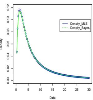
Figure 2 – Estimated density function plot for the data set-I.
Figure 4 – Estimated hazard function plot for the data set-I.
2.44, 2.58, 2.62, 2.64, 2.94, 3.03, 3.17, 3.21, 3.26, 3.39, 3.52, 3.53, 3.7, 3.76, 3.8, 3.86, 3.91, 3.96, 4.25, 4.33, 5.06, 5.07, 5.2, 5.49, 5.94, 6.77, 6.78, 6.82, 7.94, 8.05, 8.32, 8.69, 8.82, 8.85, 8.97, 9.14, 9.2, 9.7, 9.97, 10.1, 10.25, 10.27, 10.44, 10.59, 10.65, 10.75, 10.84, 11.36, 11.53, 11.55, 12.36, 13.27, 13.98, 14.01, 14.53, 16.42, 16.44, 17.07, 18.07, 18.11, 19.98, 22.21, 22.66, 23.24, 23.31, 23.8, 26.66, 29.7, 33.62, 35, 36.15, 41.75, 45.93, 50.88, 52.53, 61.31, 67.02, 67.8, 90.39, 97.82, 105.69, 114.02, 144.98, 150.84, 160.65, 239.36 Also for the simulated data, the maximum likelihood and Bayes estimates of the parameters are evaluated. The reliability and hazard estimates in both setup are also presented for t = 20 in Table 3. In table 4, the 95% asymptotic and HPD interval estimates for the parameters are provided.
5. Conclusion
In this paper, we proposed the estimation procedure for Inverse Lomax distribution under Type-I and Type-II hybrid censoring schemes. The mathematical expression for the maximum likelihood estimators and Bayes estimators are derived. The applicability of the considered model in real life has been illustrated based on bladder cancer data and simulated data and it was observed that the considered model is a good competitor of IED, GIED and ILD. Thus it can be used as a good alternative to these models whenever the situation of non-monotonicity of hazard rate is realized.
TABLE 2
Estimates of the parameters, reliability and hazard functions for different choices of censoring parameters R and T under Type-I hybrid and Type-II hybrid.
Type-I hybrid R T αˆ βˆ R(t)ˆ H(t)ˆ αˆB βˆB R(t)ˆ B H(t)ˆ B 50 2 1.2180 9.0766 0.5724 4.1128 1.3694 6.9674 0.5362 4.5663 4 1.7253 3.8813 0.4613 5.4636 1.7870 3.6601 0.4535 5.5543 10 1.7759 3.6597 0.4544 5.5470 1.8281 3.4811 0.4474 5.6253 80 3 1.5837 4.6601 0.4836 5.1930 1.6556 4.2976 0.4722 5.3260 6 1.9934 2.9189 0.4288 5.8536 2.0352 2.8265 0.4241 5.9018 10 2.1522 2.5358 0.4139 6.0297 2.1887 2.4649 0.4092 6.0743 100 5 1.7836 3.6282 0.4534 5.5591 1.8310 3.4693 0.4470 5.6300 7 1.9830 2.9504 0.4301 5.8389 2.0282 2.8440 0.4248 5.8942 12 2.2635 2.3167 0.4046 6.1378 2.3003 2.2583 0.4006 6.1754 15 2.3114 2.2328 0.4009 6.1807 2.3469 2.1748 0.3963 6.2215 120 14 2.3304 2.2011 0.3994 6.1971 2.3592 2.1535 0.3952 6.2332 17 2.3702 2.1372 0.3965 6.2306 2.4048 2.0862 0.3924 6.2673 25 2.4271 2.0516 0.3925 6.2763 2.4614 2.0043 0.3885 6.3115 Type-II hybrid 50 2 1.7759 3.6597 0.4544 5.5470 1.8275 3.4960 0.4484 5.6163 5 1.7836 3.6282 0.4534 5.5591 1.8302 3.4693 0.4469 5.6304 7 1.9830 2.9504 0.4301 5.8389 2.0217 2.8533 0.4249 5.8910 80 5 2.1522 2.5358 0.4139 6.0297 2.1924 2.4567 0.4089 6.0778 10 2.2164 2.4047 0.4084 6.0938 2.2534 2.3398 0.4040 6.1353 12 2.2635 2.3167 0.4046 6.1378 2.3020 2.2511 0.3999 6.1810 100 10 2.3114 2.2328 0.4009 6.1807 2.3489 2.1699 0.3960 6.2244 15 2.3683 2.1402 0.3966 6.2291 2.4060 2.0831 0.3922 6.2692 20 2.4090 2.0781 0.3937 6.2621 2.4453 2.0283 0.3898 6.2977 120 20 2.4297 2.0478 0.3923 6.2783 2.4695 1.9935 0.3882 6.3164 30 2.4457 2.0250 0.3912 6.2906 2.4811 1.9745 0.3869 6.3289 45 2.4567 2.0097 0.3905 6.2989 2.4948 1.9587 0.3865 6.3355
TABLE 3
Classical and Bayes interval estimates of the parameters
Type-I
Classical Interval Bayes Interval
R T αˆL αˆU λˆL ˆλU αˆL αˆU λˆL λˆU 50 2 0.4301 2.0060 0.0000 22.8656 1.1280 1.6330 4.3054 9.7186 4 0.8520 2.5985 0.7695 6.9932 1.4989 2.0598 2.8040 4.5846 10 0.9047 2.6471 0.9207 6.3986 1.5764 2.1207 2.6924 4.2232 80 3 0.7304 2.4370 0.2989 9.0213 1.3926 1.9374 3.1429 5.5161 6 1.0290 2.9577 0.8952 4.9427 1.7151 2.3334 2.2605 3.4608 10 1.1263 3.1781 0.8720 4.1997 1.8500 2.5049 1.9427 2.9574 100 5 0.9109 2.6563 0.9306 6.3258 1.5530 2.1038 2.6906 4.2327 7 1.1918 3.3353 0.8412 3.7923 1.9812 2.6458 1.8096 2.6862 12 1.2162 3.4066 0.8192 3.6465 2.0102 2.7051 1.7290 2.5852 15 1.1918 3.3353 0.8412 3.7923 1.9760 2.6357 1.8153 2.6724 120 14 1.2272 3.4336 0.8134 3.5887 2.0127 2.7088 1.7288 2.5692 17 1.2486 3.4917 0.7983 3.4762 2.0705 2.7898 1.6911 2.4969 25 1.2788 3.5753 0.7763 3.3269 2.1120 2.8482 1.6135 2.3927
Under Type-II Hybrid
50 2 0.9047 2.6471 0.9207 6.3986 1.5551 2.1058 2.6563 4.2442 5 0.9109 2.6563 0.9306 6.3258 1.5663 2.1208 2.7391 4.2382 7 1.0352 2.9307 0.9421 4.9588 1.7259 2.3129 2.3133 3.4500 80 5 1.1263 3.1781 0.8720 4.1997 1.8900 2.5372 1.9638 2.9411 10 1.1918 3.3353 0.8412 3.7923 1.9678 2.6414 1.8326 2.7161 12 1.2162 3.4066 0.8192 3.6465 2.0060 2.7040 1.7552 2.5730 100 10 1.2471 3.4895 0.7979 3.4825 2.0377 2.7439 1.6784 2.4799 15 1.2690 3.5489 0.7828 3.3734 2.0875 2.8121 1.6685 2.4463 20 1.2803 3.5792 0.7754 3.3201 2.1099 2.8298 1.6295 2.3655 120 20 1.2887 3.6028 0.7691 3.2809 2.1241 2.8594 1.6181 2.3907 30 1.2846 3.6173 0.7656 3.2741 2.1336 2.8465 1.6016 2.3229 45 1.2946 3.6187 0.7653 3.2541 2.1191 2.8482 1.5809 2.3204
TABLE 4
Estimates of the parameters, reliability and hazard functions for the simulated data set under different variations of the censoring parameters.
Under Type-I hybrid
R T αˆ βˆ R(t)ˆ H(t)ˆ αˆB βˆB R(t)ˆ B H(t)ˆ B 25 3 7.4044 0.7222 0.2310 17.1819 7.3807 0.7347 0.2301 17.1858 5 7.9984 0.6573 0.2279 17.2448 7.9436 0.6741 0.2282 17.2325 40 7 4.3176 1.4320 0.2581 16.5827 4.3592 1.4221 0.2572 16.5949 6 5.6319 1.0125 0.2428 16.9261 5.6273 1.0211 0.2416 16.9353 55 9 4.0476 1.5626 0.2625 16.4815 4.0754 1.5547 0.2618 16.4910 11 4.3525 1.4183 0.2578 16.5912 4.3863 1.4113 0.2570 16.6022 70 12 5.4655 1.0565 0.2452 16.8800 5.4919 1.0547 0.2433 16.9023 17 4.9036 1.2132 0.2508 16.7528 4.9575 1.2060 0.2496 16.7683 85 23 4.9061 1.2124 0.2508 16.7535 4.9452 1.2098 0.2499 16.7631 35 4.8896 1.2176 0.2510 16.7495 4.9226 1.2126 0.2493 16.7690 95 68 4.8681 1.2245 0.2512 16.7441 4.9025 1.2201 0.2498 16.7602 105 4.8373 1.2344 0.2515 16.7363 4.8837 1.2267 0.2501 16.7546
Under Type-II hybrid
25 3 7.9984 0.6573 0.2279 17.2448 7.9688 0.6660 0.2283 17.2349 5 10.8873 0.4562 0.2177 17.4476 10.8557 0.4590 0.2177 17.4446 40 6 4.3176 1.4320 0.2581 16.5827 4.3094 1.4303 0.2569 16.5951 7 4.8500 1.2280 0.2510 16.7452 4.8623 1.2259 0.2505 16.7495 55 9 4.3525 1.4183 0.2578 16.5912 4.3527 1.4164 0.2570 16.5992 11 5.2219 1.1194 0.2475 16.8283 5.2263 1.1178 0.2466 16.8383 70 12 4.9036 1.2132 0.2508 16.7528 4.9148 1.2098 0.2500 16.7617 17 5.0409 1.1711 0.2494 16.7864 5.0479 1.1679 0.2484 16.7974 85 23 4.9250 1.2064 0.2506 16.7583 4.9339 1.2031 0.2497 16.7684 50 4.8444 1.2321 0.2514 16.7381 4.8519 1.2307 0.2508 16.7441 95 110 4.8500 1.2303 0.2514 16.7395 4.8369 1.2285 0.2498 16.7569 150 4.8626 1.2263 0.2513 16.7427 4.8734 1.2236 0.2506 16.7495
TABLE 5
Interval estimates of the parameters for the simulated data set for different variation of R and T .
Under Type-I Hybrid
Classical Interval Bayes Interval
R T αˆL αˆU ˆλL λˆU αˆL αˆU ˆλL ˆλU 25 3 0.0000 24.4781 0.0000 2.6653 5.7423 9.3947 0.5053 0.9865 5 0.0000 26.1804 0.0000 2.3660 6.1495 9.7578 0.4545 0.8837 40 7 0.0000 14.4885 0.0000 2.8936 3.4069 5.3571 1.1927 1.6575 6 0.0000 9.9483 0.0000 3.7350 4.3994 6.9624 0.7707 1.3220 55 9 0.0000 8.9152 0.0000 3.8921 3.2880 4.9862 1.3466 1.7867 11 0.0000 9.7375 0.0000 3.5588 3.4967 5.4001 1.1680 1.6333 70 12 0.0000 13.1952 0.0000 2.8107 4.2795 6.8271 0.8052 1.3352 17 0.0000 11.3073 0.0000 3.1009 3.8830 6.1839 0.9251 1.4641 85 23 0.0000 11.2828 0.0000 3.0883 3.9083 6.0879 0.9530 1.4795 35 0.0000 11.2166 0.0000 3.0933 3.8485 6.1167 0.9611 1.4919 95 68 0.0000 11.1428 0.0000 3.1045 3.8277 6.0605 0.9576 1.4885 105 0.0000 11.0495 0.0000 3.1247 3.7760 6.0282 0.9684 1.4960
Under Type-II Hybrid
25 3 0.0000 26.1804 0.0000 2.3660 6.9636 9.0631 0.5115 0.8006 5 0.0000 41.3595 0.0000 1.8591 9.9542 11.6752 0.3512 0.5564 40 6 0.0000 9.9483 0.0000 3.7350 3.4208 5.0818 1.3246 1.5276 7 0.0000 11.6176 0.0000 3.2955 3.9994 5.8275 1.1066 1.3495 55 9 0.0000 9.7375 0.0000 3.5588 3.5131 5.1404 1.3096 1.5215 11 0.0000 12.4162 0.0000 2.9434 4.3086 6.3320 0.9838 1.2554 70 12 0.0000 11.3073 0.0000 3.1009 3.9797 5.8753 1.0842 1.3385 17 0.0000 11.7357 0.0000 3.0161 4.1779 6.0565 1.0434 1.3003 85 23 0.0000 11.3240 0.0000 3.0704 4.0253 5.8928 1.0769 1.3321 50 0.0000 11.0747 0.0000 3.1212 3.9572 5.7761 1.1092 1.3643 95 110 0.0000 11.0873 0.0000 3.1162 3.9794 5.7546 1.1029 1.3469 150 0.0000 11.1249 0.0000 3.1077 3.9280 5.7750 1.1029 1.3475
Acknowledgements
The authors would like to thank the editor and two unknown reviewers for the valuable suggestions in order to improve this manuscript.
References
A. Banerjee, D. Kundu (2008). Inference based on type-ii hybrid censored data
from a weibull distribution. IEEE Trans. Reliab., 57, pp. 369–378.
B. Chandrasekar, T. L. Alexander, N. Balakrishnan (2002). Equivariant
estimation for parameters of lomax distributions based type-ii progressively cen-sored samples. Communications in Statistics: Theory and Methods, 31, no. 10,
pp. 1675–1686.
M. H. Chen, Q. M. Shao (1999). Monte carlo estimation of bayesian credible
and hpd intervals. Journal of Computational and Graphical Statistics, 8, no. 1.
S. Chen, G. K. Bhattacharya (1988). Exact confidence bounds for an
expo-nential parameter under hybrid censoring. Comm. Statist. Theory and Method,
17, pp. 1857–1870.
A. Childs, B. Chandrasekhar, N. Balakrishnan, D. Kundu (2003). Exact
likelihood inference based on type-i and type-ii hybrid censored samples from the exponential distribution. Ann. Instit. Statist. Math., 55, pp. 319–330.
N. Draper, I. Guttman (1987). Bayesian analysis of hybrid life tests with exponential failure times. Ann. Inst. Statist. Math., 39, pp. 219–225.
S. Dube, B. Pradhan, D. Kundu (2011). Parameter estimation of the hybrid
censored log-normal distribution. J. Statist. Comput. Simul., 81, pp. 275–287.
N. Ebrahimi (1990). Estimating the parameter of an exponential distribution
from hybrid life test. J. Statist. Plann. Inference., 23, pp. 255–261.
B. Epstein (1954). Truncated life test in exponential case. Ann. Math. Statistics, 25, pp. 555–564.
K. Fairbanks, R. Madson, R. Dykstra (1982). A confidence interval for an
exponential parameter from a hybrid life test. J. Amer. Statist. Assoc., 77, pp.
137–140.
S. Geman, A. Geman (1984). Stochastic relaxation, gibbs distributions and the
bayesian restoration of images. IEEE Trans. Pattern Analysis and Machine
Intelligence, 6, pp. 721–740.
R. D. Gupta, D. Kundu (1998). Hybrid censoring schemes with exponential
failure distribution. Communications in Statistics: Theory and Method, 27, pp.
W. K. Hastings (1970). Monte carlo sampling methods using markov chains and
their applications. Biometrika, 57, no. 1.
C. Kleiber (2004). Lorenz ordering of order statistics from log-logistic and related
distributions. Journal of Statistical Planning and Inference, 120, pp. 13–19.
C. Kleiber, S. Kotz (2003). Statistical size distributions in economics and
actuarial sciences. John Wiley & Sons, Inc., Hoboken, New Jersey.
D. Kundu, B. Pradhan (2009). Estimating the parameters of the generalized
exponential distribution in presence of hybrid censoring. Communications in
Statistics: Theory and Method, 38, pp. 2030–2041.
E. T. Lee, J. W. Wang (2003). Statistical Methods for Survival Data Analysis. 3rd ed.,Wiley, NewYork.
MIL-STD-781-C (1977). Reliability design qualification and production
accep-tance test, exponential distribution. U.S. Government Printing Office,
Washing-ton, D.C.
J. Rahman, M. Aslam, S. Ali (2013). Estimation and prediction of inverse
lomax model via bayesian approach. Caspian Journal of Applied Sciences
Re-search, 2(3), pp. 43–56.
S. K. Singh, U. Singh, D. Kumar (2012). Bayes estimators of the reliability
function and parameters of inverted exponential distribution using informative and non-informative priors. Journal of Statistical computation and simulation,
83, no. 12, pp. 2258–2269.
A. F. M. Smith, G. O. Roberts (1993). Bayesian computation via the gibbs
sampler and related markov chain monte carlo methods. Journal of the Royal
Statistical Society Series B, 55, no. 1.
S. Upadhyay, N. Vasishta, A. Smith (2001). Bayes inference in life testing and
reliability via markov chain monte carlo simulation. Sankhya A, 63, pp. 15–40.
A. S. Yadav, S. K. Singh, U. Singh (2016). Bayesian estimation of lomax
distribution under type-ii hybrid censored data using lindley’s approximation method. Int. Journal of data science, x, no. x,xxxx.
Summary
In this paper, we proposed the estimation procedures to estimate the unknown parame-ters, reliability and hazard functions of Inverse Lomax distribution. The mathematical expressions for maximum likelihood and Bayes estimators are derived in presence of hy-brid censoring scheme. In most of the cases, it has been seen that maximum likelihood and Bayes estimators of the parameters are not appear in explicit form. Hence, Newton-Raphson (N-R) method has been used to draw the maximum likelihood estimates of the parameters. The Bayes estimators are obtained under Jeffrey’s non-informative prior for both shape α and scale λ using Markov Chain Monte Carlo (MCMC) technique. Further,
we have also constructed the 95% asymptotic confidence interval based on maximum like-lihood estimates (MLEs) and highest posterior density (HPD) credible intervals based on MCMC samples. Finally, two data sets have been used to demonstrate the proposed methodology.