View of Scoring ordinal variables for constructing composite indicators

SCORING ORDINAL VARIABLES

FOR CONSTRUCTING COMPOSITE INDICATORS Marica Manisera

1. INTRODUCTION

Evaluating customer satisfaction and, more generally, the quality of services on the basis of the attitudes and perceptions of individuals can be achieved by find-ing a measure of the concept of interest, i.e. a (quantitative) score for each sub-ject. Such measurement is affected by the nature of the data, usually obtained from subjective survey questions leading to “subjective” variables. When dealing with such variables, some problems can arise and affect the meaningfulness of the data. Moreover, the measurement is complex because it should take into ac-count the multidimensionality of the concept.

The individuals’ attitudes and perceptions are usually represented in the statis-tical models by latent variables or factors. Under the reflective model (Edwards and Bagozzi, 2000), the observed variables depend on the latent variables, in the sense that they are the observed effects of the latent variables, except for random er-rors. Therefore, the latent variables represent a continuum that cannot be directly observed: for this reason, data are usually collected by questionnaires with several items supposed to be related with the continuum. Responses indicate the degree of agreement with each statement, higher scores reflect greater agreement and ordi-nal variables are obtained (see, among others, Bollen, 2002).

In order to measure a p-dimensional latent variable, a questionnaire with m>p items should be administrated to n subjects and a two-step procedure should be adopted (Carpita and Manisera, 2006): (a) each observed item is transformed by a quantification or scaling or scoring procedure into a quantitative variable q that can be considered a simple indicator of the latent concept being measured; (b) the m simple indicators are then combined in order to obtain a p-dimensional com-posite indicator x representing the measure for the latent variable:

x = f (q) = 1 m j j j q =

∑

with aj'= (aj1, aj2, ..., ajp) as weights. Clearly, the composite indicator in (1) does not equal the latent variable, but is only its empirical and operational version, whose

reliability has to be checked every time with the available data set (Bollen and Lennox, 1991).

In step (a) several scoring methods, usually based on some optimality criteria, can be considered. The statistical procedure allowing the construction of com-posite indicators in step (b) can be the (un)weighted sum of the simple indicators. Both the scoring procedure and the definition of the weights should produce a composite indicator taking into account (i) the ordinal nature of the observed variables, transformed into the quantitative simple indicators; (ii) the importance of each item for the latent variable, described by the weights aj; and (iii) the mul-tidimensionality of the latent concept.

Often, the composite indicators are computed as the unweighted sum of the simple indicators: this choice is supported by practical and methodological con-siderations (Wainer, 1976). In this case, when x is p-dimensional with p>1, a very common procedure consists in assigning each item, or variable, to only one of the p dimensions, or subscales, in order to facilitate the interpretation of the compos-ite indicator x. In other words, the weights are reduced to binary weights [1,0]: when ajs equals 0, the j-th item is not relevant in the definition of the s-th subscale of the latent variable, while when ajs equals 1, the j-th item does contribute to the meaning of the s-th subscale. Moreover, if ajs = 1, then ajc = 0 for every c ≠ s, c = 1, ..., p: in fact, once the j-th item has been assigned to the s-th subscale, it cannot be assigned to another of the p subscales. For example, consider x as the composite indicator of the customer satisfaction for a certain service; each of the p>1 subscales of x is related to different aspects of the customer satisfaction for the offered service; each aspect of satisfaction is measured by one single item and, then, by the corresponding simple indicator, that contributes to the computation of only one subscale of x.

In this context, the composition of each subscale of the indicator (in terms of the contributing items) should reflect the true structure of the latent variable: a good measure of the latent variable is obtained by (1) if the assignment of items (and then of the simple indicators) to the subscales returns the true structure of the latent variable.

The objective of the present study is to investigate, by a simulation study, the impact of the scoring method on the identification of the true structure of the la-tent variable. The focus will be on a comparison of some scoring methods ap-plied to ordinal variables following a variety of distributional forms. Starting from a two-dimensional continuous latent variable with known structure, we want to inspect, by a confirmatory factor analysis, if and how much the scoring method affects the assignment of items to the two subscales of the latent variable. More-over, we want to study whether, in the presence of a multinormal latent variable, the observation of ordinal variables with a distributional form different from the “normal” one justifies the use of scoring methods taking into account the ob-served distributional form or, on the contrary, the distribution of the latent vari-able prevails over the observed distributions.

Section 2 describes the scenario in which the simulation study is defined and the five steps composing the study. In section 3 the simulation plan adopted in

the present paper is proposed, by defining all the necessary values in the scenario to make the simulation operative. The obtained results are shown in section 4. Interpretation of results, conclusions and discussion are reported in section 5. 2. THE SCENARIO

To examine the impact of the different scoring methods on the identification of the structure of the latent variables a simulation study was carried out in five steps. In the first step, population continuous data with an underlying two-dimensional continuous latent variable were created. The data were constructed starting from their correlation matrix so that a certain structure of the latent vari-able holds in the population and a model error was added.

The structure of the latent variable is defined by a prespecified correlational structure: in much detail, the construction of such data is based on an algorithm by Lin and Bendel (1985) that generates random correlation matrices for a given eigenvalue structure. Here, the correlation matrix C is defined as a block-diagonal matrix where the first block in the diagonal, C1, contains the correlations between

m1 variables and the second block in the diagonal, C2, contains the correlations between m2 variables, with m1+m2=m. The off-diagonal blocks consist of zeroes, such that the two groups of variables do not correlate with each other. Each group of variables correspond to a strong or a moderate one-dimensional eigen-value structure λi (λi with i=1,2 indicating the dominant first eigenvalue of block Ci corresponding to the i-th group of variables divided by mi). It should be noted that a necessary condition to generate one-dimensional latent trait is that all the correlations between variables are equal. This has to guarantee a dominant first eigenvalue of the correlation matrix (Meulman, 1982, p. 64). In this way, a two-dimensional latent variable, based on the multinormal distribution, underlies the data set, with m1 continuous variables forming the first dimension (or subscale) and m2 continuous variables the second dimension (or subscale) of the latent vari-able. Once generated C, the N×m data matrix H is constructed as H = BS, where B approximates an N×m orthonormal matrix (it is randomly drawn from a multinormal distribution with zero mean and variance 1/N2_{, such that B'B ≈ I)} and the m×m matrix S is given by S=WL where W and L result from the eigen-value decomposition C=WL2_{W'. The data matrix H reflects sampling variation} and H'H asymptotically equals C. In the followings, the simulated data sets with a block-diagonal correlation matrix will be called “block” data sets.

Since in the “block” data sets the two groups of variables do not correlate with each other, the two dimensions of the latent variables could be considered as separate latent variables rather than sub-dimensions of one latent variable (Bren-tari et al., 2007). In order to create a two-dimensional latent variable underlying two groups of variables with a nonzero correlation with each other, the present study also considered the simulation of “non-block” data sets following the de-scribed scheme with m2=0, then m=m1 and C=C1 having an underlying latent variable corresponding to a strong or a moderate two-dimensional eigenvalue

structure λ=[λ1,λ2]. In the generation of the “non-block” data sets, the a priori par-tition of items to the two subscales cannot be fixed by defining the variables be-longing to each of the two blocks in the correlation matrix, but has to be found by performing a two-dimensional factor analysis on the population data set and assigning items to subscales on the basis of the highest loadings.

In the second step, k samples (with n subjects) were drawn from the popula-tion data.

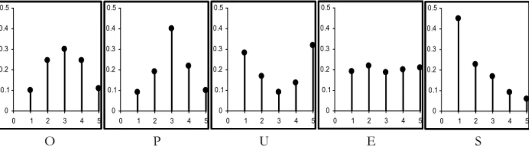
In order to reproduce the ordinal variables usually originated by questionnaires and used to construct composite indicators as in formula (1), in the third step the continuous variables were discretized, by mapping continuous intervals into points with step functions. The number of intervals and then the number of or-dered categories can be fixed at k or at kj (a different number for each variable). In the present study, five different types of discretization with k=5 were chosen, according to van Rijckevorsel, Bettonvil and de Leeuw (1985): (1) optimal (O), which follows as close as possible the normal distribution; (2) pseudo-optimal (P),

approximating O; (3) the U-shape (U), (4) the equal (E) and (5) the skew (S) types. Figure 1 displays the distributions resulting from the application of the five dif-ferent types of discretization to a simulated standard normal variable. The fre-quencies corresponding to the categories of each item for each type of discretiza-tion are obviously displayed on the y-axes.

The attempt with U, E, and S is to create distributions that, differently from O

and P, do not follow the original normal distribution, but ignore it and introduce

a bias that the quantification procedure should take into account. All the consid-ered discretizations are the result of monotonic transformations. The same dis-cretization was applied to all variables belonging to the same subscale. Therefore, 15 different combinations of discretization procedures exist when λ1=λ2 (O, P, U,

E, S, and the mixed types: i.e., the OS type means that the m1 variables are discre-tized according to O and the m2 variables according to S) and 25 when λ1≠λ2 (here, for example, OS≠SO) or when λ is a two-dimensional vector.

Figure 1 – The frequency distributions associated to the five different types of discretization.

In order to create variables which correspond to the responses given to a ques-tionnaire without any reversed item, two one-dimensional factor analyses were performed on the continuous variables belonging to each of the two subscales, in order to identify which variables have a negative loading on the found factor. The

0 0.1 0.2 0.3 0.4 0.5 0 1 2 3 4 5 0 0.1 0.2 0.3 0.4 0.5 0 1 2 3 4 5 0 0.1 0.2 0.3 0.4 0.5 0 1 2 3 4 5 0 0.1 0.2 0.3 0.4 0.5 0 1 2 3 4 5 0 0.1 0.2 0.3 0.4 0.5 0 1 2 3 4 5 O P U E S

identified variables refer to the reversed items in the questionnaire and have to be recoded.

In the fourth step, the ordinal variables were quantified. The focus in this study is on four scoring methods: (1) the optimal scaling of the categorical princi-pal component analysis à la Gifi (GI; Gifi, 1990); (2) the indirect quantification based on the Normal cumulative function (TO; Torgerson, 1958); (3) the indirect

quantification based on the negative exponential cumulative function (PO; Por-toso, 2003); (4) the linear assignment of the first positive integers to the original ordinal categories (LI), based on the hypothesis of equal distance between the

categories. Although this hypothesis is often unrealistic (see, among others, Mar-bach, 1974), we considered the linear quantification because it is widespread, in some contexts it leads to results close to the ones obtained with more refined techniques, and it constitutes the linear benchmark to evaluate the performance of the nonlinear techniques.

In the fifth step, to evaluate the impact of each scoring method on the identifi-cation of the true structure of the latent construct we used (i) the Multiple Group Method (MGM, Holzinger, 1944), (ii) the Factor Analysis (FA;Jöreskog, 1969), and

(iii) a combination of MGM and FA.

MGM is a confirmatory factor analysis approach theoretically less elegant than the well-known confirmatory factor analysis, but is very simple and in some occa-sions could be preferred (Bernstein, 1988); its performance has been studied in a recent study (Stuive et al., 2007). According to MGM, the two subscales are

de-fined, like in (1), as unweighted sums of the scores (i.e., the quantified categories) on all variables assigned to each subscale, according to the simulation scheme (for the “block” data sets) or identified by a factor analysis (for the “non-block” data sets). Next, correlations of each item with each subscale is computed. An item is expected to correlate higher with a subscale to which it is assigned in the popula-tion. If some item correlates higher with a subscales to which it is not assigned than with the subscale it is assigned to, this indicates a wrong assignment. Corre-lations were corrected for self-correlation (i.e., correCorre-lations are computed between an item and a subscale from which that item has been deleted). As in Stuive et al. (2007), corrected correlations were used to empirically verify the assignment: an assignment is correct if the assignment applied to the sample data matches the partition of items to subscales present in the population data.

FA was also used to empirically verify the assignment and, at the end, to com-pare the impact of the four scoring methods on the identification of the true structure of the latent variable. FA loadings (pattern coefficients) were used to as-sign items to the subscales of the latent variable: each item is asas-signed only to one subscale, choosing the highest loading, also when the item has a relatively high loading on both factors. Note that an adjustment has been introduced to avoid the differences in the solutions simply due to rotated solutions. Again, an assign-ment based on the FA loadings is correct if the assignment applied to the sample data matches the a priori partition of items to subscales.

Finally, we considered a combination of MGM and FA: we used the two-dimensional factor scores computed by FA (with the regression method of

Thom-son, 1951) to define the two subscales; next, like in MGM, corrected correlations

were used to empirically verify the assignment; the only difference with MGM is

then in the definition and computation of the subscales. 3. THE SIMULATION PLAN

Firstly, we generated1 _{three different “block” population data sets with} λ1=λ2=0.9, λ1=λ2=0.5, and λ1=0.9≠λ2=0.5 respectively. Each population data set counts N=500,000 observations with m1=5 and m2=5 variables.

Secondly, we fixed m2=0 and m1=m=10 and generated “non-block” population data sets (each with N=500,000 observations) with a two-dimensional eigenvalue structure defined by the vector λ=[λ1,λ2]. We decided to firstly simulate a “strong” latent variable setting λ such that λ1+λ2=0.9. A variety of couples [λ1,λ2] satisfy such condition; we chose two situations, differing in the “balance” between the two dimensions: λ=[0.45,0.45] and λ=[0.80,0.10]. Then we simulated a weaker latent variable setting λ=[0.25,0.25] and λ=[0.44,0.06] (λ1+λ2=0.5), both respect-ing the proportion between λ1 and λ2 imposed in the former “non-block” data sets.

From each data set 100 samples of n=1000 observations were drawn and we performed the MGM and the FA studies as well as the MGM-FA study, obtained by

combining MGM and FA.

With reference to the MGM and the MGM-FA study, from each data set and for

every combination of discretization and scoring procedures we computed the mean (over the 100 samples) of: (a) the proportion p of correct assignments; (b) the mean correlation µit, i=1,2; t=1,2, of the mi variables with the subscale to which they are (when i=t) or are not (when i≠t) a priori assigned to; (c) the range rit of the correlations of the mi variables with the subscale to which they are (when i=t) or are not (when i≠t) a priori assigned to; (d) the proportion pj, j=1,...,m of correct assignments for every item.

When performing the FA study, from each data set and for every combination of discretization and scoring procedures we again computed the mean of the quantities (a)-(d), but instead of the correlations of the variables with the sub-scales, we considered the loadings of the variables on the subscale to which they are (or are not) a priori assigned to.

For each simulated population data set, the best scoring method should show the highest proportion p of correct assignments; p’s being equal, the idea is that if a scoring method shows (with respect to the other scoring methods) sensibly higher µii’s, associatedto smaller rii’s, along with smaller µit’s (i≠t) associatedto higher rit’s (i≠t), then the assignment of each item to the right subscale should be easier and that scoring method should perform better than the others in allowing the correct identification of the true structure of the latent variable. Moreover, the study is suitable to reveal which type of discretization performs better for

each scoring procedure, under the assumption of a (multi)normal latent variable, suggesting whether an observed ordinal variable having a certain distributional form requires (or not) to be quantified by a specific scoring method.

4. RESULTS

Firstly, the results obtained from the analysis of the “block” data sets are pre-sented (subsection 4.1.). Then, subsection 4.2. describes the results obtained with reference to the “non-block” data sets.

4.1. The “block” data sets

The results of the MGM study applied to the “block” data set with λ1=λ2=0.9 show that in this case a preferable scoring method does not exist, and this is true for all the considered discretization types. Moreover, no distributional form re-quires to use a specific scoring method. The proportion p of correct assignments was always 1 (100%): for every combination of discretization and scoring proce-dures, all the items were assigned to the subscale to which they were a priori as-signed to. Therefore, it becomes interesting to examine the values µit and rit on which the assignment is based.

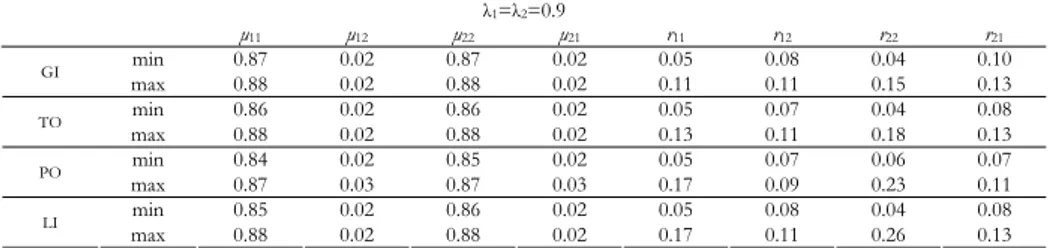
Table 1 displays the minimum and maximum values obtained across the 15 dif-ferent discretization types for the mean correlations µit with the associated ranges rit, i=1,2; t=1,2, of the mi variables with the subscale to which they were (i=t) or were not (i≠t) a priori assigned to, with reference to the considered four scoring methods. It is evident that there are no relevant differences in the results obtained by the different scoring methods, even if the PO method had slightly worse per-formances. All of them were able to correctly assign all the m items to the right subscale, µii was always very higher than µit (i≠t) and the associated ranges were always small; the intervals [min µii; max µii] and [min µit; max µit] never overlapped, making the assignment of items surely correct. Moreover, there was no discretiza-tion type performing better than the others: the detailed results are not shown, but it is clear looking at the very small differences between the minimum and maximum values of each considered parameter.

TABLE 1

MGM results for the data set with λ1=λ2=0.9: min and max of the mean correlations µit with the associated ranges

rit, i=1,2; t=1,2, of the mi variables with the subscale to which they are (i=t) or are not (i≠t) a priori assigned to,

with reference to the four scoring methods GI (Gifi), TO (Torgerson), PO (Portoso) and LI (linear assignment) λ1=λ2=0.9 µ11 µ12 µ22 µ21 r11 r12 r22 r21 min 0.87 0.02 0.87 0.02 0.05 0.08 0.04 0.10 GI max 0.88 0.02 0.88 0.02 0.11 0.11 0.15 0.13 min 0.86 0.02 0.86 0.02 0.05 0.07 0.04 0.08 TO max 0.88 0.02 0.88 0.02 0.13 0.11 0.18 0.13 min 0.84 0.02 0.85 0.02 0.05 0.07 0.06 0.07 PO max 0.87 0.03 0.87 0.03 0.17 0.09 0.23 0.11 min 0.85 0.02 0.86 0.02 0.05 0.08 0.04 0.08 LI max 0.88 0.02 0.88 0.02 0.17 0.11 0.26 0.13

The results obtained for the second “block” data set (with λ1=λ2=0.5) show correlations µ11 and µ22 smaller than in Table 1: they reflect the weaker eigenvalue structure of both groups of variables. The same holds for µ22 in the results ob-tained for the third “block” data set (λ1=0.9 and λ2=0.5), due to λ2=0.5. Again,

p=1 for every scoring method and discretization type in both data sets and the very same considerations commenting Table 1 can be repeated here.

It is interesting to note which type of discretization was associated to the minimum and the maximum values of µit. As an example, we refer to the data set simulated with λ1=0.9 and λ2=0.5, which counts 25 different combinations of dis-cretization types. For every scoring method, the minimum µ11 and µ22 corre-sponded to the data obtained when the m1 and/or the m2 variables were discre-tized according to the S discretization. The maximum µ11 appeared when the m1 variables came from the E discretization type for the GI, LI, and PO scoring

meth-ods and from the E, O, P, U discretization types for the TO scoring method. The maximum µ22 was associated with the O and P discretization types when the LI method was used, with the O type when GI was used and with the O, P, E types when TO and PO were used.

A noteworthy result is that the performance of the scoring method for each discretization type used to discretize the m1 variables was independent on the type of discretization applied to the m2 variables (and vice versa). This was also true when multivariate scoring methods were used (GI). For example, for the data set with λ1=0.9 and λ2=0.5 quantified according to the Gifi method (GI), the mean correlation µ11 of the m1 optimally discretized (O) variables with the first subscale was 0.88, whatever discretization type was chosen for the other m2 variables.

In other words, given the scoring method, the mean correlations µii of the mi variables (with the subscale to which they were a priori assigned to) were substan-tially the same when the same discretization type was applied to the mi variables. This result could be attributed to the clear separation of the two groups of vari-ables simulated in the “block” data sets.

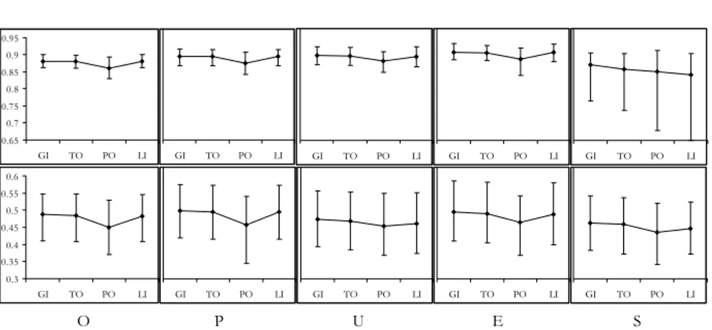
For this reason, it is possible to illustrate in one single plot the performance of the four scoring methods for each type of discretization. Figure 2 refers to the “block” data set with λ1=0.9 and λ2=0.5 and represents the mean correlations µ11 (row 1)and µ22 (row 2),with the associated ranges, of the mi variables with the subscale to which they were a priori assigned to, obtained by the four scoring methods for each discretization type (O=optimal, P=pseudo-optimal, U=U-shape,

E=equal, S=skew), where for example O includes all the combinations OO, OP, OU, OE, OS, because giving the same result.

Figure 2 shows that, given the type of discretization applied to the mi variables, µii (and rii) obtained with the four scoring methods did not notably differ (the PO

mean correlations are a little smaller). Also, the variability (and therefore the in-stability) of the results associated with the four methods did not show remarkable differences (the PO and the LI variability is a little higher). The only relevant dif-ference in the ranges associated with the correlations µii is that rii were higher when the strength of the i-th dimension of the latent variable, defined by λi, was lower (with reference to all the three “block” data sets).

Figure 2 – MGM mean correlations µ11 (row 1)and µ22 (row 2),with the associated ranges, of the mi

variables with the subscale to which they were a priori assigned to, obtained by the four scoring methods GI (Gifi), TO (Torgerson), PO (Portoso) and LI (linear assignment) for each discretization type (O=optimal, P=pseudo-optimal, U=U-shape, E=equal, S=skew), with reference to the data set with λ1=0.9 and λ2=0.5.

Both the FA and the MGM-FA results obtained for the “block” data sets con-firm the conclusions drawn from the MGM study. For all three combinations of λ1 and λ2 considered in the “block” data sets, the proportion of correct assignments was 1 for every combination of scoring method and discretization type.

With reference to the FA results obtained for the data set with λ1=0.9 and λ2=0.5, Table 2 displays the minimum and maximum values obtained across the 25 differ-ent discretization types for the mean loadings µit with the associated ranges rit, i=1,2; t=1,2, of the mi variables on the subscale to which they were (i=t) or were not (i≠t) a priori assigned to, with reference to the considered four scoring methods.

For every scoring method, the S discretization, applied to the m1 and m2 vari-ables, led to the minimum values of µ11 and µ22 respectively. The maximum value of µ11 was associated with the E discretization type for the LI and TO scoring methods, with the E, O discretization types for the GI method and with the E, O,

P, U discretization types for the PO method. The maximum µ22 was associated with the O and P discretization types when the LI method is used, with the O type when GI is used and with the O, P, E types when TO and PO are used.

TABLE 2

FA results for the data set with λ1=0.9 and λ2=0.5: min and max of the mean loadings µit with the associated

ranges rit, i=1,2; t=1,2, of the mi variables on the subscale to which they were (i=t) or were not (i≠t) a priori assigned

to, with reference to the four scoring methods GI (Gifi), TO (Torgerson), PO (Portoso) and LI (linear assignment)

λ1=0.9; λ2=0.5 µ11 µ12 µ22 µ21 r11 r12 r22 r21 min 0.88 0.01 0.56 0.02 0.03 0.06 0.16 0.07 GI max 0.91 0.02 0.59 0.02 0.14 0.1 0.19 0.08 min 0.87 0.01 0.56 0.02 0.03 0.07 0.16 0.07 TO max 0.91 0.02 0.59 0.02 0.17 0.09 0.19 0.08 min 0.86 0.02 0.54 0.02 0.06 0.06 0.18 0.07 PO max 0.89 0.02 0.56 0.02 0.22 0.09 0.22 0.1 min 0.86 0.01 0.55 0.02 0.03 0.07 0.16 0.07 LI max 0.91 0.02 0.59 0.02 0.25 0.1 0.19 0.08 O P U E S GI TO PO LI GI TO PO LI GI TO PO LI 0.65 0.7 0.75 0.8 0.85 0.9 0.95 GI TO PO LI GI TO PO LI 0.3 0.35 0.4 0.45 0.5 0.55 0.6 GI TO PO LI GI TO PO LI GI TO PO LI GI TO PO LI GI TO PO LI

The MGM-FA results obtained for the data set with λ1=0.9 and λ2=0.5 are re-ported in Table 3. It contains the minimum and maximum values obtained across the 25 different discretization types for the mean correlations µit with the associ-ated ranges rit, i=1,2; t=1,2, of the mi variables with the subscale to which they were (i=t) or were not (i≠t) a priori assigned to, with reference to the considered four scoring methods.

Again, the S discretization, applied to the m1 and m2 variables, led to the mini-mum values of µ11 and µ22 respectively. The maximum value of µ11 is associated with the E discretization type for all four scoring methods and the maximum µ22 was associated with the O and P discretization types (O, P, E when the PO method is used).

4.2. The “non-block” data sets

As already mentioned, when “non-block” data sets are simulated, the a priori partition of items to the two subscales has to be found by performing a two-dimensional factor analysis on the population data set and by assigning the items loading higher on the first dimension to the first subscale and the items loading higher on the second dimension to the second subscale.

TABLE 3

MGM-FA results for the data set with λ1=0.9; λ2=0.5: min and max of the mean correlations µit with the associated

ranges rit, i=1,2; t=1,2 of the mi variables with the subscale to which they were (i=t) or were not (i≠t) a priori assigned

to, with reference to the four scoring methods GI (Gifi), TO (Torgerson), PO (Portoso) and LI (linear assignment)

λ1=0.9; λ2=0.5 µ11 µ12 µ22 µ21 r1 r12 r2 r21 min 0.91 0.02 0.67 0.02 0.03 0.07 0.18 0.07 GI max 0.93 0.02 0.69 0.02 0.14 0.11 0.22 0.09 min 0.90 0.02 0.67 0.02 0.03 0.08 0.18 0.07 TO max 0.93 0.02 0.69 0.02 0.17 0.10 0.21 0.08 min 0.89 0.02 0.66 0.02 0.06 0.07 0.20 0.07 PO max 0.92 0.02 0.67 0.02 0.23 0.11 0.24 0.10 min 0.88 0.02 0.66 0.02 0.03 0.08 0.18 0.07 LI max 0.93 0.02 0.69 0.02 0.25 0.12 0.22 0.09

The loadings (in absolute value) of the m items on the first (l1) and on the sec-ond (l2) dimensions of the solution of the two-dimensional factor analysis per-formed on the considered “non-block” data sets are displayed in Table 4. In order to assign one item to only one subscale, for each variable the highest load-ing was chosen (see numbers in bold face in Table 4), even if the loadload-ing on the other dimension was not negligible. For example, in the data set with λ=[0.45,0.45], the 7-th item was assigned to the second subscale (l1<l2 in Table 4).

The difference with respect to the a priori partition set in the generation of the “block” data sets is remarkable: we substantially force the loadings to be binary. This makes the match between the assignment in the sample data and the a priori partition of items much more difficult.

TABLE 4

Loadings (absolute value) of the m items on the first (l1) and on the second (l2) dimensions of the solution of the

two-dimensional factor analysis performed on the “non-block” data sets generated with different vaues of λ

λ=[0.45, 0.45] λ=[0.80, 0.10] λ=[0.25, 0.25] λ=[0.44, 0.06] item l1 l2 l1 l2 l1 l2 l1 l2 1 0.00 0.93 0.78 0.52 0.24 0.56 0.52 0.37 2 0.18 0.91 0.17 0.92 0.14 0.57 0.35 0.52 3 0.91 0.22 0.78 0.52 0.57 0.11 0.36 0.45 4 0.76 0.54 0.91 0.24 0.31 0.53 0.32 0.58 5 0.89 0.31 0.87 0.33 0.43 0.46 0.37 0.46 6 0.78 0.52 0.86 0.37 0.30 0.54 0.50 0.40 7 0.64 0.69 0.68 0.65 0.59 0.24 0.55 0.32 8 0.00 0.93 0.53 0.78 0.22 0.56 0.50 0.40 9 0.59 0.72 0.86 0.37 0.54 0.26 0.45 0.44 10 0.89 0.30 0.54 0.76 0.65 0.00 0.55 0.31

Nevertheless, the results of the MGM study applied to the “non-block” data set

with λ=[0.45, 0.45] show a proportion p of correct assignments equal to 1 (100%) for every combination of discretization and scoring procedures. Given the scor-ing method, the mean correlations of each group of variables with the correct subscale were substantially the same when the same discretization type is applied to those variables, independently on what discretization type was applied to the other group of variables. This is surprising, because in the “non-block” data sets the two groups of items are not well separated as in the “block” data sets. More-over, this can not be attributed to the equal weight in λ of the two dimensions of the latent variable, because it happened for every other “non-block” data set con-sidered in this paper. Figure 3 is the analogous of Figure 2 and shows the mean correlations µ11 (row 1)and µ22 (row 2),with the associated ranges, of the mi vari-ables with the subscale to which they were a priori assigned to, obtained by the four scoring methods for each discretization type.

Figure 3 – MGM mean correlations µ11 (row 1)and µ22 (row 2),with the associated ranges, of the mi

variables with the subscale to which they were a priori assigned to, obtained by the four scoring methods GI (Gifi), TO (Torgerson), PO (Portoso) and LI (linear assignment) for each discretization

type (O=optimal, P=pseudo-optimal, U=U-shape, E=equal, S=skew), with reference to the data set

with λ=[0.45, 0.45]. O P U E S GI TO PO LI GI TO PO LI GI TO PO LI GI TO PO LI GI TO PO LI GI TO PO LI GI TO PO LI GI TO PO LI 0.55 0.6 0.65 0.7 0.75 0.8 0.85 0.9 GI TO PO LI 0.55 0.6 0.65 0.7 0.75 0.8 0.85 0.9 GI TO PO LI

Once again the four scoring methods showed similar results. The main differ-ence with the “block” data set analysed by Figure 2 is that the mean correlations obtained in the “non-block” data were associated with a higher variability; this is probably due to the rule used to a priori partition the items.

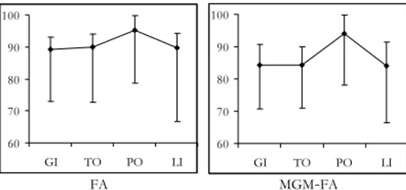
Unlike the MGM, the FA and the MGM-FA applied to the “non-block” data set with λ=[0.45, 0.45] revealed a proportion p of correct assignments lower than 1 for many combinations of discretization types, for every scoring method. Figure 4 shows the mean value of p along with the associated range, computed across the 25 combinations of discretization types for the four scoring methods.

Figure 4 – Mean value (dot) and range of p, computed across the 25 combinations of discretization

types, obtained by the FA (left-hand side) and the MGM-FA (right-hand side) studies applied to the data set with λ=[0.45, 0.45].

It is worthy to note that the minimum p was associated with the S

discretiza-tion type, when applied to both groups of variables, for every scoring method. Moreover, the main responsible for the wrong assignments was the 7-th item: it was always associated with the minimum mean pj (p per item), and this is due to the cross-loading observed in Table 4.

The proportion p of correct assignments for the other three “non-block” data sets was lower than 1 for many combinations of discretization types, for every scoring method. Figure 5 represents the mean value of p along with the associated range, computed across the 25 combinations of discretization types for every scoring method. Since the comparison among different confirmatory factor analysis is not the objective of the present study, Figure 5 compacts the results only showing the MGM-FA results; we chose to represent them because they are

similar to the FA results and worse than the MGM results, in the sense that the MGM-FA study always reported lower means of p with larger associated ranges than the MGM results.

The results obtained for the “non-block” data set with λ=[0.80,0.10] show that the LI scoring method gave mean p’s more instable than the other scoring

meth-ods. The mimimum mean p obtained by the LI method was 44.3% and was asso-ciated with the S discretization type. Once excluded that value, the second

mini-mum was higher (67.5%, associated to the SP discretization type), but still respon-sible for a higher instability. We could expect that the LI method does not per-form well with skewed ordinal variables, but here every scoring method gave minimum p’s associated with a discretization combination including the S type.

FA MGM-FA 60 70 80 90 100 GI TO PO LI 60 70 80 90 100 GI TO PO LI

Moreover, for every scoring method the 7-th item was often wrong assigned and this is due to the cross-loading observed in Table 4. In this case, all the other items were nearly always correctly assigned (94.48% was the minimum pj with j≠7 for every study – MGM, FA and MGM-FA – and for every scoring method).

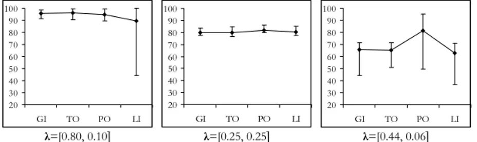
Figure 5 – Mean value (dot) and range of p, computed across the 25 combinations of discretization

types, obtained by the MGM-FA study applied to the “non-block” data sets with λ=[0.25, 0.25]

(left-hand side), λ=[0.80, 0.10] (centre), λ=[0.44, 0.06] (right-(left-hand side).

With reference to the “non-block” data set with λ=[0.25,0.25], Figure 5 shows that the mean p’s and the corresponding ranges did not sensibly vary across the scoring methods. The minimum and the maximum p’s were not associated with the same discretization type for every scoring method: for example, in the MGM

-FA study, the minimum p’s were associated with OU when the variables are scored

by GI, with PU when TO is applied, with UO when PO is applied an with PE when

LI is applied. A rule determining those associations was not easy to find. On the

other side, for every scoring method the 5-th item was often wrong assigned: it is always associated with the minimum mean pj (again, a cross-loading can be ob-served in Table 4).

Also, Figure 5 shows that, with reference to the “non-block” data set with λ=[0.44, 0.06], the PO scoring method provided higher mean p’s but associated

with larger ranges. Here, the PO method also differs from the other methods be-cause the minimum p’s were found when the U discretization was applied, while

the minimum p’s of the other scoring methods were associated with the S discre-tization type.

5. CONCLUSIONS AND DISCUSSION

In order to construct composite indicators like (1) measuring latent variables, for example customer satisfaction or, more generally, the quality of services per-ceived by individuals, it is important to choose the more appropriate scoring method to transform all the observed items into the quantitative variables that are then combined to construct the composite indicators.

Assuming that the composite indicators are computed as the unweighted sum of those quantitative variables, when x is p-dimensional with p>1, each item has

λ=[0.80, 0.10] λ=[0.25, 0.25] λ=[0.44, 0.06] 20 30 40 50 60 70 80 90 100 GI TO PO LI 20 30 40 50 60 70 80 90 100 GI TO PO LI 20 30 40 50 60 70 80 90 100 GI TO PO LI

to be assigned to only one of the p subscales. The present study investigated the impact of the choice of the scoring method on the construction of indicators: by a simulation study, population data with a known structure of the latent variable, given by a fixed a priori partition of the items, have been generated, and the im-pact of the scoring method on the correct (or incorrect) assignment of the items to the subscales has been evaluated.

Both “block” and “non-block” population data sets showed that it is difficult, among the four considered methods, to find a scoring method performing better than the others: if the objective is to identify the true assignment of items to the subscales of a latent variable, we could say that a preferable scoring method does not exist, and this holds for all the considered discretization types.

With the caution due to the small differences in the results regarding the four scoring methods, especially in the analysis of the “block” data sets, it seems that in the presence of skewed variables, all the scoring methods perform worse than in the presence of the ordinal variables obtained by the other discretization types. This could be due to the fact that the characteristics of the normal latent variable is not well recovered by a skewed ordinal variable.

In the “block” data sets, the PO scoring method had very slightly worse

per-formances, and this was true also in the presence of skewed variables. Moreover, the analysis of the “block” data sets showed that the ranges associated with the correlations µii were higher when the strength of the latent variable, defined by λi, was lower. Therefore, it seems that when the latent variable is very strong, the choice on the scoring method is still more negligible.

In the “non-block” data sets, the PO scoring method had worse performance if

the focus is on µii and rii, while when the focus is on p’s, because they are lower than 1, sometimes it performed slightly better than the others.

The LI scoring method often gave the more unstable results.

A noteworthy result is that the performance of the scoring method for each discretization type used to discretize the m1 variables was independent on the type of discretization applied to the m2 variables (and vice versa). This was also true when multivariate scoring methods were used (GI).

This result holds independently from the eigenvalue structure of the involved groups of variables. Therefore, it is a result that could be attributed not only to the block structure of the correlation matrix, which makes the groups of variables uncorrelated and the two dimensions of the latent variables well separated. In fact, this holds also for the “non-block” data sets, independently of the strength of the latent variable and from the balance between the two dimensions of the latent variable.

Future research involves the comparison of the different scoring methods when the latent variable underlying the data is not multinormal and is not sym-metrical. The main difficulty in writing such new simulation programs refers to the opportunity of generating multivariate data sets with underlying multivariate latent variables following certain distributional forms.

Someone could argue that it is important to avoid the use of simulation stud-ies. In the present paper, we had to use simulation: by definition latent variables

are not observable, and the structure of a latent variable cannot be known, unless it is set in a simulation study. This reminds another limit of the present study: la-tent variables could also have a distributional form different from whatever simu-lated model, but it is again not observable.

The construction of composite indicators of customer satisfaction and of the quality of a service takes advantage from the results of the present simulation study. In fact, they show that, under the assumption of a (multi)normal latent variable and the here considered conditions, there is no scoring method perform-ing better than the others for each type of discretization. This is true also for the skewed ordinal variables: the scoring method (PO) that specifically takes into ac-count the distributional form of the ordinal variable is not able to perform better than the other methods if the latent variable is symmetrical. The different eigen-value structures set in the population data sets allow to understand that the strength of the latent variable does not have influence on the choice of the scor-ing method.

In conclusion, the present study indicates that, under the considered condi-tions, if the objective of the research is to assign items to subscales of a latent variables in order to define composite indicators as in (1), complex scoring pro-cedures are not always the best choice to quantify ordinal variables and that it is advisable to use simpler methods, perhaps except for the linear assignment of the first positive integers to the original ordinal categories, which in our simulations resulted the more unstable method in many occasions.

Department of Quantitative Methods MARICA MANISERA

University of Brescia

ACKNOWLEDGEMENT

The author wish to thank M. Linting and B.J. van Os from Leiden University for the valuable discussions regarding the first step of the simulation study.

REFERENCES

I.H. BERNSTEIN,(1988), Applied multivariate analysis, Springer, New York.

K.A. BOLLEN, (2002), Latent variables in psychology and the social sciences, “Annual Review of

Psy-chology”, 53, pp. 605-634.

K.A. BOLLEN, R. LENNOX,(1991), Conventional wisdom on measurement: a structural equation

perspec-tive,“Psychological Bulletin”, 110, pp. 305-314.

E. BRENTARI, S. GOLIA, M. MANISERA,(2007), Models for categorical data: a comparison between the

Rasch model and Nonlinear Principal Component Analysis,“Statistica & Applicazioni”, V, 1, pp. 53-77.

M. CARPITA, M. MANISERA, (2006), Un’analisi delle relazioni tra equità, motivazione e soddisfazione per

il lavoro. In M. Carpita, L. D’Ambra, M. Vichi, G. Vittadini (Eds.), Valutare la qualità. I servizi di pubblica utilità alla persona. Guerini editore, Milano, pp. 311-360.

J.R. EDWARDS, R.P. BAGOZZI, (2000), On the nature and direction of relationships between constructs

and measures, “Psychological Methods”, 5, pp. 155-174.

A. GIFI,(1990), Nonlinear multivariate analysis, Wiley, Chichester.

K.J. HOLZINGER, (1944), A simple method of factor analysis, “Psychometrika”, 9, pp. 257-262. K.G. JÖRESKOG, (1969), A general approach to confirmatory maximum likelihood factor analysis,

“Psychometrika”, 34, pp. 183-202.

S.P. LIN, R.C. BENDEL, (1985), Algorithm AS213: Generation of population correlation on matrices

with specified eigenvalues, “Applied Statistics”, 34, pp. 193-198.

G. MARBACH, (1974), Sulla presunta equidistanza degli intervalli nelle scale di valutazione, “Metron”,

XXXII, n. 1-4.

J.J. MEULMAN, (1982), Homogeneity analysis of incomplete data, DSWO Press, Leiden.

G. PORTOSO,(2003), L’esponenziale e la normale nella quantificazione determinata indiretta; un

indica-tore d’uso, “Rivista Italiana di Economia Demografia e Statistica”, LVII, pp. 135-139.

I. STUIVE, H.A.L. KIERS, M.E. TIMMERMAN, J.M.F. TEN BERGE,(2007), A comparison of methods for

em-pirical verification of assignment of items to subtests, University of Groningen, Submitted for

publication.

G.H. THOMSON,(1951),The factorial analysis of human ability, London University Press,

Lon-don.

W.S. TORGERSON,(1958), Theory and methods of scaling, Wiley, New York.

J. VAN RIJCKEVORSEL, B. BETTONVIL, J. DE LEEUW, (1985), Recovery and stability in nonlinear PCA,

Dept. of Data Theory, Univ. of Leiden, RR-85-21.

H. WAINER, (1976), Estimating coefficients in linear models: it don’t make no nevermind,

“Psycho-logical Bulletin”, 83, pp. 213-217.

SUMMARY

Scoring ordinal variables for constructing composite indicators

In order to provide composite indicators of latent variables, for example of customer satisfaction, it is opportune to identify the structure of the latent variable, in terms of the assignment of items to the subscales defining the latent variable. Adopting the reflective model, the impact of four different methods of scoring ordinal variables on the identifica-tion of the true structure of latent variables is investigated. A simulaidentifica-tion study composed of 5 steps is conducted: (1) simulation of population data with continuous variables measuring a two-dimensional latent variable with known structure; (2) draw of a number of random samples; (3) discretization of the continuous variables according to different distributional forms; (4) quantification of the ordinal variables obtained in step (3) accord-ing to different methods; (5) construction of composite indicators and verification of the correct assignment of variables to subscales by the multiple group method and the factor analysis. Results show that the considered scoring methods have similar performances in assigning items to subscales, and that, when the latent variable is multinormal, the distri-butional form of the observed ordinal variables is not determinant in suggesting the best scoring method to use.