Università Degli Studi Di Macerata Dipartimento Di Economia E Diritto
Corso Di Dottorato Di Ricerca In Metodi Quantitativi Per La Politica Economica
Ciclo XXX
NONLINEAR DYNAMICS AND ECONOMIC GROWTH.
THE INFLUENCE OF ELASTICITY OF SUBSTITUTION BETWEEN INPUT FACTORS AND DIFFERENTIAL SAVINGS PROPENSITIES.
RELATORE DOTTORANDO
Chiar.mo Prof. CRISTIANA MAMMANA Dott. FRANCESCA GRASSETTI
COORDINATORE
Chiar.mo Prof. MAURIZIO CIASCHINI
Contents
1 Introduction 4
2 Measures of elasticity of substitution and equilibrium levels associated to
attrac-tors 9
2.1 Preliminaries . . . 9
2.2 Definitions . . . 11
2.2.1 Attractors and equilibrium levels . . . 11
2.2.2 Attractors and elasticity of substitution . . . 12
2.2.3 Measures of elasticity of substitution and capital per-capital level on the at-tractors . . . 13
2.3 Application on Kaldor model . . . 14
2.3.1 Existence and stability of attractors . . . 14
2.3.2 Elasticity of substitution associated to the attractors. Measures . . . 16
3 Long run dynamics of Kaldor model with Shifted Cobb-Douglas technology 21 3.1 The economic setup . . . 21
3.2 Long run dynamics . . . 25
3.2.1 Existence of equilibrium levels . . . 25
3.2.2 Stability of equilibrium levels . . . 28
3.3 Complex attractors . . . 30
3.4 Further developments . . . 33
4 Long run dynamics of Kaldor model with Kadiyala technology 34 4.1 The economic setup . . . 34
4.2 Boundedness of growth path . . . 36
4.3 Long run dynamics . . . 41
4.3.1 Existence of equilibrium levels . . . 41
4.3.2 Stability of equilibrium levels . . . 43
4.4 Complex attractors . . . 45
5 Conclusions 50
Abstract
This thesis investigates the qualitative and quantitative dynamics of the Solow-Swan growth model with di↵erential saving considering di↵erent production functions in order to analyse how the long run behaviour of the economy is influenced by the elasticity of substitution between production factors and by di↵erent savings propensity between workers and shareholders. In the first chapter the economic growth problem of establishing a relation between the elasticity of substitution, capital and output per-capita levels when dealing with a non constant elastic-ity of substitution production function is discussed. Starting from a discrete-time setup, some definitions of elasticity of substitution associated to an attractor are proposed and a method to measure it is suggested. The main goal is to compare dynamic growth models with VES, sigmoidal and CES production functions. To this end, the method proposed is applied to the Kaldors model using a VES production function with constant returns to scale. It is found that when simple dynamics are exhibited, a country characterized by production functions with higher elasticity of substitution experiences higher capital and output per-capita equilibrium levels. On the other hand, when the long term dynamics consist of cycles or more complex fea-tures, then an ambiguous relation between elasticity of substitution and asymptotic dynamics is shown. In the second chapter the Kaldor growth model is analysed, assuming the Shifted Cobb-Douglas (SCD) production function, a technology that - di↵erently from CES and VES one - allows one to consider the dynamics of non developed and developing countries as well as that of developed economies. The resulting model is a discontinuous map generating a poverty trap. Furthermore multistability phenomena may emerge: next to the vicious circle of poverty, long run behaviours may include boom and bust periods (fluctuations may arise when the elasticity of substitution is lower than one) and convergence to a positive level of capital per-capita. In the last chapter the discrete time neoclassical one-sector growth model with di↵erential savings is studied assuming the Kadiyala production function which shows a variable elasticity of substitution symmetric with respect to capital and labor. It is shown that, if workers save more than shareholders, then the growth path is bounded from above and the boundary is independent from of the savings rate of shareholders. The growth path for non-developed countries is influenced only by the savings rate of shareholders while level of capital per capita of developed economies is influenced by the savings rate of workers. More-over, multistability phenomena may occur so that the model is able to explain co-existence of under-developed, developing and developed economies. Fluctuations and complex dynamics may arise when the elasticity of substitution between production factors is lower than one and shareholders save more than workers.
1
Introduction
In the classic article A Contribution to the Theory of Economic Growth [67], the Nobel Prize-winning Robert M. Solow investigated the relationship between the structure of production functions and income distribution. Solow proposed a model describing the dynamics of the physical capital and the long-term evolution of the growth process taking into consideration the role of capital, labour and technology. In his essay he took into consideration how the long-run equilibrium or disequilibrium of the economy changes considering di↵erent types of production functions: the Harrod-Domar, the Cobb-Douglas (CD) and a third type of production function that five years later had been generalized with the two-factor Constant Elasticity of Substitution (CES) production function (see Solow et al. [4]). He refuted the Harrod-Domar assumption of fixed proportions (see Harrod [32] and Domar [28]) and supposed the possibility of substituting labour for capital in production (see Solow [67]). This assumption has led the way to investigations of how the elasticity of substitution a↵ects capital and output equilibrium levels and hence economic growth. When the Cobb-Douglas production function is considered, the model monotonically converges to the steady state, since the elasticity of substitution between production factors is constant and equal to one.
Notice that elasticity of substitution between production factors measures how quickly the marginal rate of technical substitution of labour for capital changes as we move along an isoquant. The greater the ease with which one factor can be substituted for another (for a given level of output), the greater will be the elasticity of substitution. In linear production functions inputs are perfectly substitutable for each other, isoquants are straight lines and = +1. On the contrary, in fixed-proportions production functions inputs are perfect complements, isoquants are L-shaped and = 0. Many papers investigating neoclassical growth model used the CD specification of the production function in which capital and labour can be substituted for each other and the elasticity of substitution is equal to one. More recently, several contributions investigated theoretically and empirically the role played by the CES production functions (see Klump and Preissler [43], Klump and de La Grandville [42], Miyagiwa and Papageorgiou [53] and Masanjala and Papageorgiou [47]) in which elasticity of substitution between inputs is constant and takes values that are either greater or lower than one. Although CES production functions widen the range of values of the elasticity of substitution from 0 to1, these production functions restrict to be constant along an isoquant whereas the elasticity of substitution between inputs should be a variable depending upon output and factor combinations (see Hicks [33], Allen [2] and Revankar [63]). Moreover, for more than two factors, di↵erent degrees of substitutability between inputs are not allowed (see the Impossibility theorem of Uzawa [75] - McFadden [48]). The class of Variable Elasticity of Substitution (VES) production functions proposed by Lu and Fletcher [45], Revankar [62] and Sato and Ho↵man [66] fix this criticisms exhibiting an elasticity of substitution between capital and labour that is a↵ected by changes in the economy’s per-capita capital level. Many studies analyzed the role of a variable elasticity of substitution within the Solow model (see Karagiannis et al. [40], Papageorgiou and Saam [55]).
In 1989 de La Grandville considered the Solow model with a normalized CES function (equal to a in the third case presented in Solow’s work) and showed that an higher elasticity of substitution implies an higher capital per-capita level and he conjectured that the huge growth in Japan and East Asian countries could had been due to an higher elasticity of substitution between capital and
labour instead of a more efficient technical progress or an higher savings rate. Rainer Klump and Olivier de La Grandville considered a Solow type growth model and a normalized CES production function and demonstrated that an economy with higher elasticity of substitution experiences a higher level of per-capita income, both in transition and in steady state (Klump and La Grandville [42]). They compared economies characterized by the same growth model and CES production function, di↵erentiated only by the degree of elasticity of substitution.The same result was found by Klump and Preissler [43].
In line with these researches Miyagiwa and Papageorgiou used the CES production function in the Diamond overlapping-generation model (see Diamond [26]) to study economic growth and its relation with elasticity of substitution between production factors (see Miyagiwa and Papageorgiou [53]). Di↵erently from the other works, they found that, if capital and labour are relatively substi-tutable, an higher elasticity of substitution between production factors leads to a lower output per worker, both in transition and in steady state. They concluded that whether the economic growth is positively or negatively a↵ected by the elasticity of substitution between production factors it depends on the used setup, i.e. the Solow or the Diamond framework.
Recently several papers have considered the Solow-Swan model with Constant Elasticity of Sub-stitution (CES) or the Variable Elasticity of SubSub-stitution (VES) production functions, in order to analyze the long-run dynamics of the system when the elasticity of substitution is lower then one, greater then one or even non constant (for CES see Brianzoni et al. [14, 18], Masanjala and Papageorgiou [47] and Papageorgiou and Saam [55] while for VES see Brianzoni et al. [19] and Karagiannis et al. [40]). Most of the cited works found that fluctuations and even more complex dynamics may arise if the elasticity of substitution is sufficiently low. Evidently the elasticity of substitution between production factors plays a crucial role in the theory of economic growth. Moreover it represents one of the determinants of the long-run equilibrium level (for the correlation between elasticity of substitution and capital per-capita levels see Klump and La Grandville [42] and Miyagiwa and Papageorgiou [53]).
It is easy to see that accurate connection between endogenous economic growth and elasticity of substitution can be determined when a framework with a CES production function is proposed. In this case it is possible to investigate both long run dynamics and the relationship between elasticity of substitution and economic growth. Di↵erently, with Variable Elasticity of Substitution produc-tion funcproduc-tions such as the VES producproduc-tion funcproduc-tion or the sigmoidal one, even if the qualitative and quantitative long term dynamics have been widely studied, no attention has been paid to the relation between variable elasticity of substitution and growth. This limitation is due to the fact that with VES or other non-constant elasticity of substitution production functions the elasticity itself depends on the level of capital per-capita. In fact, once we define the elasticity of substitution as a variable depending on capital or output, the methodology used with CES production function to investigate its relationship with economic growth loses e↵ectiveness. More precisely, with CES production functions one investigates how the elasticity of substitution influences the long term capital per-capita levels. Di↵erently, with VES or sigmoidal production functions this relation is altered, since the same elasticity of substitution is a↵ected by the capital per-capita levels. Hence, we pass from a unilateral a↵ect system ( ! kt) to a bilateral a↵ect system ( $ kt), where is
the elasticity of substitution between production factors while ktrepresents the capital per-capita
The choice to investigate the behaviour of the growth model considering a Variable Elasticity of Substitution production function is due to the fact that many empirical studies prove that VES (instead of CES) production functions are a better representation of reality. In 1968, Lovell [44] rejected both the Cobb-Douglas and the CES specifications in favor of the VES production function using data for two-digit U.S. manufacturing industries; the same result was obtained by Diwan [27] for individual U.S. manufacturing firms, by Revankar [63] for the private non-farm sector of the U.S and by Meyer and Kadiyala [50] using agricultural data. Evidences in favor of the VES production function are also provided for Japanese (see Bairam [8] and Sato and Ho↵man [66]) and Soviet (see Bairam [7]) economies, as well as for larger region data (see Karagiannis et al. [40]). All these contributions uphold that the VES production function is a better representation of the elasticity of substitution.
As a further step on the economic growth theory Kaldor ([38, 37]) proposed a Solow’s type growth model in which the two income groups (labor and capital) might have di↵erent savings behaviour. Consequently the investigation of the influence of di↵erential savings rates between workers and shareholders arises in literature. B¨ohm and Kaas [12] studied the Kaldor model assuming a generic production function satisfying the weak Inada conditions and showed that instability, fluctuations and complex dynamics may emerge. Recently Brianzoni et al. [14, 15, 18] investigated Kaldor’s growth model in discrete time with di↵erential savings and endogenous labour force growth rate while assuming a CES production function. They found that the model can exhibit cycles or even chaotic dynamic patterns. Moreover, Cheban et al. [22] investigated the neoclassical growth model with the labour force dynamics described by the Beverton-Holt equation (see [9]) assuming a CES production function. In both contributions the authors found that if the elasticity of substitution is positive but sufficiently low, the economic patterns are bounded, and, if the elasticity of sub-stitution is close to zero, the economic system can converge to a steady state characterized by no capital accumulation. Tramontana et al. [72] used the Leontief production function and proved that cycles and fluctuation can be exhibited if shareholders save more than workers. As a further step in this field, the role of di↵erent VES production functions has been considered: Brianzoni et al. [19] studied Kaldor model with Revankar [63] production function; they found that unbounded endogenous growth is possible (di↵erently from CES) and fluctuations may arise if shareholders save more than workers and the elasticity of substitution between production factors falls below one. Similar results can be found considering non-concave production functions (see Brianzoni et al.[16] and Michetti [51]).
As Azariadis and Stachurski [6] showed, concave neoclassical growth models don’t take in consid-eration the di↵erences production technology between rich and poor countries while non-concave growth models may generate persistent-poverty aggregate income data. In order to take into ac-count the existence of poverty trap (the condition for which a ac-country need a critical level of physical capital before a growth dynamic could be observed), recently Brianzoni et al. [16] considered a non-concave production function. Also for non developed or developing countries complicated dynamics emerge if the elasticity of substitution is sufficiently low confirming that the elasticity of substitu-tion is responsible for the creasubstitu-tion and propagasubstitu-tion of complexity.
In the first part of this work a way to establish a relation between the elasticity of substitution between production factors and the long term growth dynamics when dealing with a non-constant
elasticity of substitution production function is suggested. While with CES production functions, whatever the attractor, the elasticity between production factors is a constant, with VES or sig-moidal production functions depends on the output kt and hence on the long term dynamics
exhibited by the model, fixing a contrast in measuring the output variation depending on the elas-ticity of substitution. The method introduced will be used to analyze the relation between the elasticity of substitution and capital per-capita levels considering Kaldor’s growth model [37] and the Variable Elasticity of Substitution (VES) production function in intensive form with constant return to scale, as given by Revankar (see Revankar [62] and Karagiannis et al. [40]). The purpose is also to verify whether the main result obtained by Klump and La Grandville [42] using the CES function still holds, i.e. if greater elasticity of substitution implies higher equilibrium levels also with VES, so as to extend the study in Brianzoni et al. [19]. It is demonstrated that, when the long run dynamics are simple, then there exists a positive correlation between elasticity of substitution, capital and output per-capita associated to the attractor. On the other hand, when the economic patterns exhibit cycles or more complex dynamics, an ambiguous relation between elasticity of substitution and the asymptotic dynamics is shown.
In the second part of this work the discrete time one-sector Solow-Swan growth model with dif-ferential savings as given by B¨ohm and Kaas [12] is studied while assuming that the technology is described by the Shifted Cobb-Douglas (SCD) production function as proposed by Capasso et al. [20]. As in Brianzoni et al. [16, 17] the use of a non-concave production function states the ex-istence of a poverty trap. Notice that whereas CES and VES production functions well describe developed economies but they are not able to explain dynamics related to non developed countries, the SCD production function implies a minimum level of physical capital essential for production, a requirement of capital needed in order to observe increasing returns. This kind of production function is often considered in literature in order to describe the growth dynamics of developing countries. Indeed, as Azariadis and Stachurski [6] thoroughly explain, poor economies are often characterized by market failure, inefficient practices, ”institution failure” and also social norms and conventions which cause the well know ”vicious circle of poverty”. This considerations make the model economically significant in order to analyze the growth dynamics of developing countries: can a poor economy escape from poverty trap? Which is the required initial investment? If a developing country has passed the poverty trap just now, could it’s economy fall down again into it? We shall try to answer these questions.
From the mathematical point of view, when the SCD production function is considered the re-sulting model is described by a discontinuous map, a type of framework recently considered in several economic models (see, among all, B¨ohm and Kaas [12] and Tramontana et al. [72, 74, 73]) since recent mathematic tools allow to investigate economic phenomena defined by discontinuous systems. The main goals are to describe the qualitative and quantitative long run dynamics of the growth model and to evaluate the relation between elasticity of substitution and capital per-capita equilibrium levels in not well developed countries. The results of the analysis show that complex dynamics, multistability phenomena and non-connected basin of attraction may emerge. Moreover, as in Klump and La Grandville [42], a positive correlation between elasticity of substitution and long term dynamics is exhibited.
The third part of this work extends previous literature on economic growth by examining the neoclassical one-sector growth model with di↵erential savings while assuming that technology is described by the Kadiyala [36] production function: a VES production function whom property
is to present elasticity of substitution symmetric with respect to input factors, fixing monotony’s critic moved to main VES functions. The aim of the work is to investigate how the elasticity of substitution between capital and labour and savings rate of capitalists (shareholders) and workers influence the speed with which economies grow, the existence of poverty traps and the occurrence of fluctuating long run behaviours.
It is found that when the elasticity of substitution between labour and capital is lower than one the growth path for non-developed countries is influenced only from investments made by capitalist while for developed economies the level of capital increase only for higher values of the savings rate of workers.
As in Chakraborty [21] poverty traps may result if savings and investment rates are low despite the absence of inefficient technology, mainly considered the source of ”vicious circle of poverty” (see among all Capasso et al. [21] and Azariadis and Stachurski [6]).
In addition qualitative and quantitative dynamics of the model are analyzed: multistability phe-nomena, fluctuation and complex dynamics can be observed if elasticity of substitution is lower than one, confirming results obtained with di↵erent technologies.
This work is organized as follow: in the first chapter of this study the definitions of single-value measures associated to an attractor are proposed and a method to measure the elasticity of substi-tution associated to an attractor is suggested. It is highlighted how this technique make it possible to compare models with VES, sigmoidal and CES production functions. The relation between elas-ticity of substitution and capital per-capita equilibrium levels considering Kaldor’s model with VES production function [62] is investigated by using both analytical tools and numerical techniques; to this aim the new measuring method proposed is applied. In the second chapter the Kaldor model with Shifted Cobb-Douglas is presented and its proprieties are discussed. The existence and the stability of the steady states are analyzed and the possibility of multiple equilibria, complex dynamics and also complex basins are demonstrated. In the third chapter the influence of savings rates on the growth path of the Kaldor model with Kadiyala production function is analyzed. The dynamical behaviour of the framework is investigated and complex dynamics and multistability phenomena are discussed. Chapter 5 conclude the work.
2
Measures of elasticity of substitution and equilibrium
lev-els associated to attractors
2.1
Preliminaries
Consider a discrete time setup in which kt=KLtt 0 is the capital per-capita at time t2 N, where
Kt is the stock of capital and Lt is the labour force. Let (kt) : R+ ! R be the elasticity of
substitution between production factors, that is, if f (kt) :R+! R is the production function, then
(kt) represents a measure of the ease with which capital and labour can be substituted in f (kt).
More precisely (kt) represents the elasticity of output per-capita with respect to the marginal
product of labour (see Hicks [33] and Robinson [65]). Notice that if (kt) is continuous and twice
di↵erentiable, then (kt) is calculated as follows (see Sato and Ho↵man [66]):
(kt) =
f0(k
t)[f (kt) f0(kt)kt]
f (kt)f00(kt)kt
. (1)
As an example, if f (kt) is of CES type, i.e. f (kt) = (1 + ktp)
1
p, then (k
t) = 1 p1 8kt 0, that is
the elasticity of substitution between production factors does not depend on the capital per-capita level. Di↵erently, if f (kt) has a di↵erent form, then (kt) could no longer be constant. Consider,
for instance, the following functions.
(i) The VES production function proposed by Revankar is given by: f (kt) = Akat[1 + bakt]1 a, A > 0, 0 < a < 1, b 1, 1 kt b (2) hence (kt) = 1 + bkt (3)
(it has been considered in growth models such as in Brianzoni et al. [19], Cheban et al. [22], Karagiannis et al. [40] and Grassetti et al. [29]).
(ii) The SIGMOIDAL production function can be formalized as: f (kt) = ↵kpt 1 + ktp , ↵ > 0, > 0, p 2 so that (kt) = 1 + pkpt p(1 kpt) (1 + k p t) (4) (this function has been used in growth models such as in Capasso et al. [20], Brianzoni et al. [16], Michetti [51] and Brianzoni et al. [17]).
In both cases (i) and (ii), is a function of kt.
capital per-capita kt, t2 N (and consequently of output yt= f (kt)). For instance one can consider
the Solow-Swan growth model given by
kt+1= (kt) = 1
1 + n[(1 )k + sf (kt)]
where n 0 is the constant population growth, 2 (0, 1) is the depreciation rate of capital and s2 (0, 1) is the constant saving rate (see [67], [53], [55] and [16]); or the more recent Bh¨om and Kaas Solow-Swan growth model with di↵erential savings given by
kt+1= (kt) = 1
1 + n[(1 )kt+ sw(f (kt) ktf
0(k
t)) + srktf0(kt)]
(see [38], [37], [56], [12], [18], [19], [51] and [17]) where sw and sr are respectively the savings rate
of workers and shareholders.
In all these cases the one dimensional map kt+1 = f (kt) describing the evolution of capital
per-capita over time depends on both the per-capital per-per-capita and the elasticity of substitution between production factors, i.e. kt+1= (kt, (kt)). Given function f , the main focus of economic growth
studies is to investigate the long term dynamics produced by (kt) for a given initial state k0> 0.
By following Medio and Lines [49], we recall the definition of an attractor for a discrete time dynamic system.
Definition 2.1. Let ⌦ be the state space and define !(x) as the set of all !-limit points of x for a map. A compact invariant subset of the state space ⇤⇢ ⌦ is said to be an attractor if
(i) its basin of attraction, or stable set, B(⇤) ={x 2 ⌦ | !(x) ⇢ ⇤}, has strictly positive Lebesgue measure;
(ii) there is no strictly smaller closed set ⇤0⇢ ⇤ so that B(⇤0) coincides with B(⇤) up to a set of
Lebesgue measure zero.
In particular, if we consider the map kt+1 = (kt), where the state space is given by R+, then
the attractor ⇤ can be a fixed point (therefore ⇤ = k⇤), or it can be a n-cycle (so that ⇤ = c n =
{k⇤
1, k⇤2, . . . , kn⇤}), or a more complex set. If limt!1ft(k0) = +1 8k0 2 I(k0, r)\ R+, then we
state ⇤ = (1).
Consider ⇤ = k⇤ and assume that (k
t) = 8kt, that is the elasticity of substitution between
production factors is constant. Then if the capital per capital level increases (decreases) when the elasticity of substitution increases, i.e. @k@⇤( ) > 0 (resp. <), we can conclude that the elasticity of substitution between production factors positively (resp. negatively) a↵ects the capital per-capita equilibrium value8k02 B(k⇤). However, if ⇤ is not a fixed point, then a first question that arises
is how to measure the attractor of f . Secondly, if di↵erent attractors coexist, each one with its own basin, a second question that arises is which attractor must be considered in order to establish the relation between and ⇤. Finally, the most important question to be considered is how to inspect the relation between elasticity of substitution and long term growth dynamics when also depends on kt. In what follows we will suggest a way to tackle these questions. Recall that the
elasticity of substitution between inputs measure the ease in which capital can be substituted by labour in production. Therefore, during boom and bust periods, the measures we will define in the following can be used by governments to evaluate economic policies able to reallocate resource between inputs with the purpose of reducing costs while avoiding losses in production.
2.2
Definitions
In this section some definitions are given in order to measure the asymptotic states and the elasticity of substitution associated to an attractor in an economic growth model and explain their relation.
2.2.1 Attractors and equilibrium levels
Recall that the economic growth model is given by kt+1 = (kt, (kt)), therefore - whichever the
production function (whether a constant or a non-constant elasticity of substitution production function) - the capital per-capita at time t + 1 is equal to (kt, (kt)). The prevailing interest is to
inspect the long term dynamics of the economic growth model, that is to investigate the structure of the attractor of map f in the long term for an economic meaningful initial capital per-capita level k0> 0.
When the attractor is a fixed point ⇤ = k⇤, the measure of the long term capital per-capita level is
basic and exact being, indeed, equal to the fixed point itself. However, when the attractor consists of a more complex set, as a cycle or a complex attractor, its measure is not so immediate. Therefore, we propose a method to measure the attractor of the dynamic system using a synthetic one-value index.
Definition 2.2. Let kt+1 = (kt, (kt)), f : A ✓ R+ ! R+ be a discrete time one-dimensional
system describing the evolution of capital per-capita kt, where (kt) is the elasticity of substitution
depending on kt and t2 N.
• If the attractor is ⇤⇤ = k⇤, then the measure of capital per-capita level associated to the
attractor is
k⇤⇤ = k⇤.
• If the attractor is ⇤1 = +1, then the measure of capital per-capita level associated to the
attractor is
k⇤1= +1.
• If the attractor is a periodic cylce ⇤cn = cn = {k1⇤, k⇤2, . . . , kn⇤}, then three measures of the
capital per-capita level associated to the attractor can be given: – the maximum capital per-capita level associated to ⇤cn
kM ⇤cn = max{k⇤i : ki⇤2 ⇤cn}; – the minimum capital per-capita level associated to ⇤cn
km⇤cn = min{ki⇤ : k⇤i 2 ⇤cn}; – the average capital per-capita level associated to ⇤cn
¯ k⇤cn = 1 n n X i=1 ki⇤, ki⇤2 ⇤cn.
• If the attractor is a complex set, then it can be described by the following set ⇤cx={ki : ki= f
i(k
0), N p i N, k02 B(⇤cx)} .
i.e. ⇤cx is given by the last p k values obtained by iterating the system N times (where N p are conveniently chosen, sufficiently high natural numbers) and three measures of capital per-capita level can be associated to the attractor:
– the maximum capital per-capita level associated to ⇤cx kM ⇤cx = max{ki : ki2 ⇤cx}; – the minimum capital per-capita level associated to ⇤cx
km⇤cx = min{ki : ki2 ⇤cx}; – the average capital per-capita level associated to ⇤cx
¯ k⇤cx = 1 p N X i=N p ki, ki2 ⇤cx.
With the previous definitions we established a method to measure the long term capital per-capita equilibrium in the case in which the attractor is a fixed point or a cycle or a more complex set. In the same line, we now expound how to measure the elasticity of substitution by taking into account the long term dynamics of the growth model.
2.2.2 Attractors and elasticity of substitution
As for the long term capital per-capita equilibrium, a measurement issue arises when attempting to measure the non-constant elasticity of substitution associated to an attractor. Also when measuring the elasticity of substitution between production factors one face a hurdle when the dynamics of the economic growth model are analyzed and the elasticity of substitution is associated to an attractor that may be complex. Recalling definition 2.2, the following definition determines a method to measure the elasticity of substitution associated to an attractor in the case in which function depends on the capital per-capita level.
Definition 2.3. Let kt+1= (kt, (kt)) be a discrete time one-dimensional system describing the
evolution of capital per-capita and consider definition 2.2.
• If the attractor is a fixed point k⇤, the elasticity of substitution associated to the attractor is ⇤⇤ = (k⇤⇤) (where k⇤⇤ = k⇤) ;
• If the attractor is ⇤1= +1, the elasticity of substitution associated to the attractor is ⇤1 =klim
t!+1 (kt)
• If the attractor is a n-cycle, three measures of elasticity of substitution can be associated to the attractor:
– the maximum elasticity of substitution associated to ⇤cn
M ⇤cn = max{ (ki⇤) : k⇤i 2 ⇤cn}; – the minimum elasticity of substitution associated to ⇤cn
m⇤cn = min{ (ki⇤) : k⇤i 2 ⇤cn}; – the average elasticity of substitution associated to ⇤cn
¯⇤cn = 1 n n X i=1 (k⇤i), k⇤i 2 ⇤cn.
• If the attractor is a complex set, three measures of elasticity of substitution can be associated to the attractor:
– the maximum elasticity of substitution associated to ⇤cx
M ⇤cx = max{ (ki) : ki2 ⇤cx}; – the minimum elasticity of substitution associated to ⇤cx
m⇤cx = min{ (ki) : ki2 ⇤cx}; – the average elasticity of substitution associated to ⇤cx
¯⇤cx = 1 p N X i=N p (ki), ki2 ⇤cx.
Since the elasticity of substitution seems to be a determinant of economic growth, we fixed the fundamentals to compare how the elasticity of substitution a↵ects the growth process when a VES instead of CES production function is considered.
2.2.3 Measures of elasticity of substitution and capital per-capital level on the at-tractors
One of the fundamental topics linked to the research on economic growth models is to inspect how the elasticity of substitution a↵ects the capital per-capita equilibrium level. As seen, the elasticity of substitution between production factors is given by (12). Consider a CES production function, then (kt) = 8kt 0 that is the elasticity of substitution does not depend on kt.
Therefore, it is easy to verify what occurs to long term dynamics (and hence to economic growth) when varying the elasticity of substitution (se [42], [43] and [53]). What is the relation between
elasticity of substitution and the long term dynamics of economic growth models when a non-constant production function is considered?
We take as examples the elasticity of substitution as given in (3) and (4): (kt) = 1 + bkt and (kt) = 1 +
pktp
p(1 ktp) (1 + ktp)
.
In both cases depends on k and some parameters of interest (b or p and respectively). Given an economic growth model (kt, ) and an elasticity of substitution function (kt, ) (where is the
parameter of interest while the other parameters are fixed), the previous definitions can be used as follows.
• Once the attractor ⇤ is determined, the capital per-capita level associated to the attractor k⇤ can be obtained.
• Furthermore, the elasticity of substitution associated to the attractor (⇤) can be computed 8 2 I ✓ R (where I is the set of values that can assume, according to the hypothesis of the model).
• Finally it is possible to verify if - when is moved - k⇤ and ⇤ move in the same direction,
so that k⇤ and ⇤ are positively correlated, or if k⇤ and ⇤ move in the opposite directions,
so that k⇤and ⇤ are negatively correlated.
2.3
Application on Kaldor model
Thanks to the definitions given above, we can now analyze the relation between the elasticity of substitution between production factors, long term dynamics and economic growth when a produc-tion funcproduc-tion with non-constant elasticity of substituproduc-tion is taken into account. In this secproduc-tion we present an applied example. In Brianzoni et al. [19] the dynamics of Kaldor’s growth model with VES production function have been studied. The authors found all the attractors of the model and demonstrated that complex dynamics may arise if the elasticity of substitution is positive and lower than 1. However, they did not investigate the correlation between elasticity of substitution and capital per-capital equilibrium levels nor the implication on economic growth.
2.3.1 Existence and stability of attractors
In this section we briefly recall both the economic setup and outcomes achieved by Brianzoni et al. [19], in order to better explain how the new procedure herewith proposed can be applied. Consider Kaldor’s [37] model, where workers and shareholders have di↵erent but constant saving rates. The one-dimensional map describing the evolution of capital per-capita is given by
kt+1=
1
1 + n[(1 )kt+ sww(kt) + srktf
0(k t)]
where 2 (0, 1) is the depreciation rate of capital, sw 2 (0, 1) and sr 2 (0, 1) are respectively
the constant savings rates for workers and shareholder, n > 0 is the constant population growth rate and t 2 N. Wage rate w(kt) equals the marginal product of labour while the total capital
income per worker of a shareholder is given by ktf0(kt). Furthermore, consider the Revankar [62]
production function, that is a VES production function, given by (2), where A > 0, 0 < a < 1, b 1 and k1t b.
When b > 0 the final growth model describing the capital per-capita evolution is given by H(kt) = 1 1 + n ⇢ (1 )kt+ A ✓ kt 1 + abkt ◆a [sw(1 a) + sr(a + abkt)] (5)
which is strictly increasing with respect to kt. Di↵erently, when 1 b < 0 the final growth model
is given by (kt) = ( H(kt) 8kt2 [0, 1b] H( 1b) 8kt> 1b (6) that is a continuous and piecewise smooth map, nonlinear for kt2 [0, 1b] and with a flat branch
for kt > 1b. Furthermore the elasticity of substitution between production factors is defined in
(3). In what follows we briefly recall the main results reached in Brianzoni et al. [19].
Remark 2.4. Consider the economic growth model be given by H or F defined in (5) and (6). (1) If b > 0, then:
(i) when n+
A > (ab) aas
rb, H has one stable fixed point given by kt = k⇤ > 0 and one
unstable fixed point given by kt= 0;
(ii) when 0 < n+A < (ab) aas
rb, H has a unique, unstable, fixed point given by kt= 0.
(2) If b 2 [ 1, 0), F has a non-di↵erentiable point given by P = 1 b, F ( 1 b) . Given M = sr b a 1 s2 w(1 a)+asr(sw sr) (sw asr)a and N = sw[ b(1 a)] 1 a, then: (a) Consider sr< sw,
(i) if n+A 2 [0, M), F has one unstable fixed point given by k = 0 and one superstable fixed point given by k⇤= F ( 1
b);
(ii) if n+
A 2 (M, N), F has two unstable fixed points given by k = 0 and k⇤22
⇣ sr bsw, 1 b ⌘ , one locally stable fixed point given by k⇤12
⇣ 0, sr
bsw ⌘
and one superstable fixed point given by k⇤= F ( 1
b);
(iii) if n+A > N , F has one unstable fixed point given by k = 0 and one locally stable fixed point given by k1⇤2
⇣ 0, sr bsw ⌘ . (b) Consider sr sw (i) if n+
A 2 [0, N), F has one unstable fixed point given by k = 0 and one superstable
fixed point given by k⇤= F ( 1 b);
(ii) if n+A > N , F has one unstable fixed point given by k = 0 and one positive fixed point given by k⇤2 0, 1
· if 1 b < F 1 b , k⇤ is superstable; · if 1 b > F 1
b , k⇤ may be unstable and complex dynamics may be exhibited.
Now that we have recalled the results obtained by Brianzoni et al. [19] on local and global dynamics, we can move on to our study to verify how the elasticity of substitution a↵ects Kaldor’s growth model with VES production function.
2.3.2 Elasticity of substitution associated to the attractors. Measures
In this section we want to establish if, when complex attractors emerge, the capital per-capita equi-librium level and the elasticity of substitution associated to the attractor are positively correlated, negatively correlated or not correlated. From Brianzoni et al. [19] we know that, when b2 [ 1, 0) and sr sw, if n+A > N and 1b > F 1b , then the positive fixed point may lose stability, so the
economy fluctuates and cycles or more complex dynamics can be exhibited.
In order to analyze the attractors of map F while moving b, we proceed by making use of numerical experiments. Therefore, we fix all the parameters in F except for parameter b by considering the values available from international economic databases. For parameters s (saving rate) and n (exogenous labour growth rate) we consider the values given by OECD1, Eurostat2 and World
Bank3 for the annual saving rate from 1995 to 2014 (excluding negative values, as the growth
model requires). For parameter A (total factor productivity index) we consider the estimate given by OECD4from 1993 to 2014. Therefore, the following table of admissible values for the parameters
is assumed.
Parameter Range value
Saving rate s2 [0.00015, 0.59] Labor growth rate n2 [0.00002, 0.27346] Total factor productivity A2 [56.8, 106]
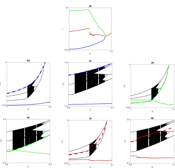
We fix A = 57, n = 0.2, sw= 0.01 and sr= 0.05. Moreover we set a = 0.85 and b2 [ 0.6, 0.2) in
order to assure that conditions (b.ii) of Remark 2.4 are satisfied. As it has been proved in Brianzoni et al. [19], in this case complex dynamics may occur, as we can observe in Figure 1.
We can now use the definitions given in section (2.2.1) to measure the attractors of the dynamic system. Figure 2 panel (a) shows the maximum capital per-capita level (blue line), the minimum capital per-capital level (green line) and the average capital per-capita level (red line) associated to the attractor.
1For saving rate see ”OECD (2016), Saving rate (indicator). doi: 10.1787/↵2e64d4-en”; for labour growth rate
see ”OECD (2016), Labour force (indicator). doi: 10.1787/ef2e7159-en”.
2For saving rate see ”Eurostat, Household saving rate, code: tsdec240”; for labour growth rate see ”Eurostat,
LFS main indicators, code: lfsi-act-a”.
3For saving rate see ”Gross savings, World Bank national accounts data, Catalog Sources: World Development
Indicators”; for labour growth rate see ”Labor force, International Labour Organization using World Bank population estimates, Catalog Sources: World Development Indicators”
Figure 1: Bifurcation diagram w.r.t. b.
Thanks to the graphical analysis we can observe that the minimum capital per-capita level associ-ated to the attractor increases as parameter b increases. For the maximum capital per-capita level associated to the attractor, a change in the curve slope can be observed in correspondence with the border collision bifurcation5, as it can be seen in Figure 2 panel (b). In Figure 2 panel (d),
the behaviour of the average capital per-capita level associated to the attractor can be observed: an increasing trend is visible in the sequence of the period doubling bifurcation cascade. We can conclude that, where a trend is visible, the capital per-capita level increases as the parameter asso-ciated to the elasticity of substitution is increased.
It is of importance to highlight that we are in a simplified state of definition (2.3), being the elasticity of substitution given by (3) a linear function; indeed the following proposition holds.
Proposition 2.5. Let (kt) be a linear function of ktand let the elasticity of substitution associated
to an attractor ⇤ be as defined in (2.3). Then:
• M ⇤cn = (kM ⇤cn);
• m⇤cn = (km⇤cn);
• ¯⇤cn = (¯k⇤cn);
• M ⇤cx = (kM ⇤cx);
Figure 2: Bifurcation diagram w.r.t. b and maximum (blue), minimum (green) and average (red) capital per-capita level associated to the attractor.
• m⇤cx = (km⇤cx);
• ¯⇤cx = (¯k⇤cx).
Proof. Being the elasticity of substitution a linear function, for every set K ={k1, k2, . . . kn} and
S ={ 1, 2, . . . , n} (with i= (ki), ki2 K), • max{ i2 S} = (kM)|kM 2 K being kM ki 8ki2 K; • min{ i2 S} = (km)|km2 K being km k 8ki2 K; • ¯ = (¯k), where ¯ = 1 n Pn
i=1 i and ¯k = 1nPni=1ki.
In Figure 3 panel (a) the behaviour of the elasticity of substitution associated to the attractor can be observed.
Figure 3: Maximum (blue), minimum (green) and average (red) elasticity of substitution and capital per-capita level (dashed) associated to the attractor.
Following the definitions given in proposition 2.5, we show the maximum elasticity of substitution associated to the attractor ( M ⇤) (blue line), the minimum elasticity of substitution associated
to the attractor ( m⇤) (green line) and the average elasticity of substitution associated to the
attractor (¯⇤) (red line). We can observe the relation between the capital per-capita level and
the elasticity of substitution associated to the attractor when moving parameter b. As far as the maximum capital per-capita level and its elasticity of substitution are concerned, in Figure 3 panel (b) it can be observed that both values increase when moving parameter b. A di↵erent behaviour is exhibited for the minimum capital per-capita level associated to the attractor and its elasticity of substitution, as it is shown in Figure 3 panel (d): a negative correlation between the two values is visible along the path until the border collision bifurcation occurs. Lastly, in Figure 3 panel (d), the
relation between average capital per-capital level and the associated elasticity of substitution can be observed. Similarly to the minimum capital per-capita level a negative correlation is exhibited up to the border collision bifurcation. Notice that when the attractor is a fixed point, maximum, minimum and average capital per-capita level coincide and a positive correlation is shown.
To summarize, we disclose a numerical simulation in order to analyze the relation between the capital per-capita level associated to the attractor and the elasticity of substitution, when map F exhibits cycles and more complex dynamics. We observe that the maximum, minimum and average capital per-capita level associated to the attractor increase as the parameter b is increased. Furthermore, we find a positive correlation between maximum capital per-capita level associated to the attractor and its elasticity of substitution. This result is similar to that obtained by Klump and La Grandville [42] using a CES production function in the Solow model: if two economies di↵er only for the level of their elasticity of substitution, the economy with the higher elasticity of substitution will have the higher capital per-capita level in the steady state. Conversely from Klump and La Grandville [42], a negative correlation between minimum and average capital per-capita level associated to the attractor and their elasticity of substitution is shown along the path.
3
Long run dynamics of Kaldor model with Shifted
Cobb-Douglas technology
3.1
The economic setup
Consider the discrete time neoclassical one-sector growth model as proposed by B¨ohm and Kaas [12]: following Kaldor [38, 37] and Pasinetti [56] workers and shareholders have di↵erent but constant saving rates (respectively sw and sr), the labour force grows at rate n and is the depreciation
rate of capital. Moreover, shareholders receive the marginal product of capital f0(k) and the total
capital income per worker is kf0(k). We assume that the wage rate equals the marginal product of
labor, that is
w(k) = f (k) kf0(k). (7)
Following B¨ohm and Kaas [12], the map describing the capital accumulation over time t 2 N is given by kt+1= (kt) = 1 1 + n[(1 ) kt+ sww(kt) + srktf 0(k t)] , kt 0 (8)
where n 0, 2 (0, 1], sw 2 (0, 1) and sr 2 (0, 1). Following Capasso et al. [20] we consider
a Shifted Cobb-Douglas (SCD) production function that is a continuous concave and non-di↵erentiable production function stating the existence of a critical level of capital needed before to get returns. This production function, di↵erently from concave ones, well describes also non-developed countries since it takes in consideration the realistic need to establish a basic structure for production (as machineries and infrastructures) in order to obtain output. The SCD production function in its intensive form is given by
f (kt) =
(
0 0 kt kc
A(kt kc)↵ kt> kc
(9) where A > 0 is the total productivity factor and 0 < ↵ < 1 is the output elasticity of capital. kc 0
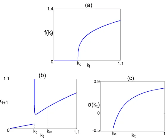
is the critical level of capital per-capita delimiting the poverty trap, that is the minimum capital per-capita initial level causing increasing returns since, when a country with almost no physical capital is considered, an initial investment is required before production (see Figure 4 (a)).
Notice that if kc ! 0+, then f (kt) approaches the Cobb-Douglas production function, therefore
f (kt) can be considered as a generalization of the well-known Cobb-Douglas production function.
Moreover f0(kt) = ( 0 0 < kt< kc ↵A(kt kc)↵ 1 kt> kc .
In order to assure non-negative wage and the framework having an economic meaning we assume that if f (k) kf0(k) < 0 then the resulting wage is equal to zero, hence
w(kt) =
(
0 0 kt kw
A(kt kc)↵ 1[(1 ↵)kt kc] kt> kw
Figure 4: Common parameter values: n = 0.3, = 0.4, sw = 0.6 and sr = 0.7. (a) SCD
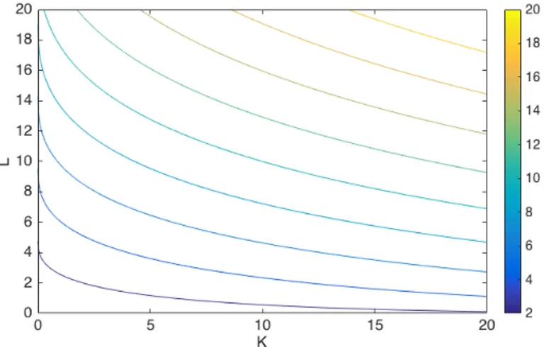
production function. Parameter values: ↵ = 0.3, A = 1.2 and kc = 0.4. (b) The final map for
capital accumulation. Parameter values: ↵ = 0.5, A = 2.122 and kc = 0.4. (c) The elasticity of
substitution. Parameter values: ↵ = 0.3, A = 1.2 and kc= 0.2.
where kw= 1 ↵kc > kc. Taking into account equations (8), (9) and (10), the final one dimensional
map describing the capital per-capita evolution is given by:
kt+1= (kt) = 8 > > < > > : 1 1+nkt 0 kt kc 1 1+n[(1 )kt+ A↵srkt(kt kc) ↵ 1] k c< kt kw 1 1+n n (1 ) kt+ Asw(kt(kktc)+↵(skc)1r↵sw)kt o kt> kw . (11)
We now discuss the main properties of map (kt), i.e. the Solow-Swan growth model in the
form given by B¨ohm and Kaas [12] with SCD as proposed by Capasso et al. [20]. Map is non negative, defined in R+ and it is discontinuous in kt = kc since limkt!kc (kt) =
1
1+nkc and
limkt!k+
c (kt) = +1, while it is continuous in kw being limkt!kw (kt) = limkt!k+w (kt) =
1 1+n h 1 1 ↵kc+ A ⇣ ↵ 1 ↵kc ⌘↵i
for any fixed value of kt, the capital per-capita level at time t + 1 is always negatively influenced
by the labour force growth rate (n) and the depreciation rate of capital ( ), whereas - passed the poverty trap i.e. kt< kc- it is positively a↵ected by the total productivity factor (A). Furthermore,
for well developed countries, i.e. kt > kc with k high enough, the higher the di↵erence between
workers and shareholders saving rates, the higher the capital per-capita at time t + 1.
Recall that the elasticity of substitution between production factors for nonlinear production func-tion is defined as follows (see Sato and Ho↵man [66]):
(kt) = f 0(k
t)[f (kt) f0(kt)kt]
f (kt)f00(kt)kt
. (12)
and it is the measure of the ease in which capital and labour can be substituted in production. Being
f00(kt) = A↵(↵ 1)(kt kc)↵ 2 kt> kc
and being = +1 for linear production functions, the elasticity of substitution between production factors for the SCD can be easily calculated and it is given by
(kt) = ( +1 0 < kt< kc 1 kc (1 ↵)kt kt> kc .
Observe that f (kt) belongs to the class of Variable Elasticity of Substitution (VES) production
functions, as (kt) depends on the level of capital per-capita kt. Moreover (kt) is
discontinu-ous in kt = kc being limkt!kc (kt) = +1 whereas limkt!k+c (kt) =
↵
1 ↵ < 0. Furthermore
limkt!+1 (kt) = 1. Notice that if kt> kw > kc then (kt) > 0, whereas if kc < kt < kw then (kt) < 0 (the graph of (kt) is in Figure 4 (c)). Notice also that is always lower then 1 for
kt> kc. For what it concerns the sign of we observe that even if a negative elasticity of
substitu-tion between producsubstitu-tion factors is not convensubstitu-tional, several producsubstitu-tion funcsubstitu-tions in literature show negative elasticity of substitution (see Prywas [59], Andrikopoulos et al. [3], Thompson and Taylor [71], Nguyen and Streitwieser [54], Stern [68], Hamilton et al. [31] and Jurgen [35]), for instance, as suggested by Paterson [57], a negative elasticity of substitution can occur if complementary in-puts are considered. Therefore, a negative elasticity of substitution between production factors for kc < kt< kwsuggests that in the early stages of production, immediately outside the poverty trap,
capital and labour are complementary and not replaceable.
As it has been discussed, map is defined in R+ and it is discontinuous in kt= kc. Map = 0 i↵
kt= 0, hence it passes through the origin. This is a trivial condition for economic growth models as
no capital can be produced without capital. Moreover, map is always not negative. For kt kc,
map is a linear function passing through the origin with slope m = 1
1+n. Note that m is positive
and lower then 1, moreover it increases as or n decreases. Firstly we compute the derivative for map that is given by
0(k t) = 8 > > < > > : 1 1+n kt< kc 1 1+n n 1 + ↵Ahsr(↵kt kc) (kt kc)2 ↵ io kc< kt< kw 1 1+n n 1 + ↵Ahsr(↵kt kc)+(1 ↵)swkt (kt kc)2 ↵ io kt> kw . (13)
Notice that is non-di↵erentiable in kw and hence if an attractor A exists and kw2 A its stability
must be discussed separately. For what it concerns the behaviours of map for sufficiently high levels of capital per capita we observe that8k > kc function may be strictly decreasing or it may
present a turning point, i.e. a minimum point, as the following proposition states. Proposition 3.1. Let as given by (11). Assume kp= ↵sr+(1 ↵)ssrkc w and v =
1
A . Then function
is unimodal for kt> kc with minimum point kmin.
Proof. We define the function G(k) = ( sr↵(k kc)↵ 1 kc < k kw sw(k kc)+↵(sr sw)k k(k kc)1 ↵ k > kw (14) where G0(k) = ( sr↵(↵ 1)(k kc)↵ 2 kc< k < kw (↵ 1)[sw+(sr sw)↵]k2+(2 ↵)swkck swk2c k2(k kc)2 ↵ k > kw (15)
For k > kc function may be written in terms of function G defined in (14) as follows
(k) = 1 1 + n{(1 )k + AkG(k)} k > kc (16) hence 0(k) = 1 1 + n{1 + A[G(k) + kG 0(k)]} k > k c, k6= kw (17) Then 0(k) = 0 i↵ G(k) + kG0(k) = 1
A . Observe that G(k) + kG0(k) can be written as follows:
H(k) = G(k) + kG0(k) = (
sr↵(↵k kc)(k kc)↵ 2 kc< k < kw ↵{[sw+(sr sw)↵]k srkc}
(k kc)2 ↵ k > kw hence the turning points of are solutions of
H(k) = 1
A . (18)
Function H(k) is such that limk!k+
c H(k) = 1, moreover H0(k) = ( sr↵(↵ 1)(↵k 2kc) (k kc)3 ↵ kc< k < kw ↵(1 ↵){(2sr sw)kc [(1 ↵)sw+↵sr]k} (k kc)3 ↵ k > kw . Assume kp=↵sr+(1 ↵)ssrkc w and z = sr(2↵ 1) ⇣ ↵ 1 ↵kc ⌘↵ 1 . We first consider solutions of equation (18) for k2 (kc, kw):
(i) for ↵ > 1
2, function H(k) < 0 i↵ kc < k < kc
↵, therefore H(k) can intersect the constant and
negative function v = 1
A only in the interval I1= kc, kc
↵ . Moreover H0(k) > 08k 2 I1and
limk!kc ↵
H(k) = 0. So that H(k) = v has always one solution; (ii) for ↵1
2, function H(k) < 08k 2 (kc, kw) = I2, H0(k) > 08k 2 I2and limk!kwH(k) = z, so that H(k) = v has one solution in the interval I2 if v z;
We now consider solutions of equation (18) for k > kw:
(iii) for ↵ < sr sw
2sr sw and sr> sw, function H(k) < 0 for k2 (kw, kp) = I3, moreover limk!k+wH(k) = z + (1 ↵)sw ⇣ ↵ 1 ↵kc ⌘↵ 1 , limk!kp H(k) = 0 and H0(k) > 08k 2 I 3 so that H(k) = v has
one solution in the interval I3if v z + (1 ↵)sw
⇣ ↵ 1 ↵kc ⌘↵ 1 . Since z < z + (1 ↵)sw ⇣ ↵ 1 ↵kc ⌘↵ 1
cases (ii) and (iii) can not occur simultaneously, and hence at most one turning point may exists for ↵ < sr sw
2sr sw. Notice that for z < v < z+(1 ↵)sw ⇣
↵ 1 ↵kc
⌘↵ 1
equation (18) has no solution. Nevertheless for these parameter values it has limk!kwH0(k) < 0
and limk!k+ wH
0(k) > 0 and hence (k) is unimodal with minimum point k
min = kw.
Note that if condition (i) holds then kmin < k↵c, if condition (ii) holds then kmin kw while if
condition (iii) holds then kmin2 (kw, kp). In all other cases kmin = kw.
3.2
Long run dynamics
In this section we consider the question of the existence of steady states of system (11) and then we discuss about the local stability.
3.2.1 Existence of equilibrium levels
The problem of finding the number of steady states is not trivial to solve, considering the high number of parameters. As a general result, the map always admits one fixed point characterized by zero capital per capita, i.e. k = 0 is a fixed point for any choice of parameter values. Anyway, steady states which are economically interesting are those characterized by positive capital per worker. As previously underlined is a discontinuous map. Moreover, no positive fixed point exists for 0 < kt kc, being 0 <1+n1 < 1. In order to determine the positive fixed points of with kt> kc
we consider function G as given in (14). The positive steady states of map are the solutions of equation
G(kt) = n +
A . (19)
The following proposition concerning the number of steady states of the Solow growth model with SCD and di↵erential saving can be proved.
Proposition 3.2. Let as given by (11). Define g =n+A and kM = kc
(2 ↵)sw+p↵sw[(4sr 3sw)↵ 4(sr sw)]
2(1 ↵)[sw+(sr sw)↵] .
(i) Assume sr sw. Then has two fixed points given by kt= 0 and k⇤> kc. Moreover
(a) if g G(kw), k⇤ kw;
(b) if g < G(kw), k⇤> kw.
(ii) Assume sr< sw. Then
(a) if g > G(kM) there exist two fixed points given by kt= 0 and k⇤< kw;
(b) if g = G(kM) there exist three fixed points given by kt= 0, k1< kw and k2= kM;
(c) if G(kM) < g < G(kw) there exist four fixed points given by kt = 0, k1 2 (kc, kw),
k22 (kw, kM) and k32 (kM, +1);
(d) if g = G(kw) there exist three fixed points given by kt= 0, k1= kw and k2> kM;
(e) if g < G(kw) there exist two fixed points given by kt= 0 and k⇤> kM.
Proof. kt= 0 is a solution of equation kt= (kt) for all parameter values hence it is a fixed point
for all parameter values. Being 1
1+n < 1, for all 0 < kt kc map does not intercept the main
diagonal. Function G is such that G(kt) > 08kt > kc, furthermore limkt!k+c G(k) = +1 while limkt!1G(kt) = 0. G(kt) is continuous in kwbeing limkt!kwG(kt) = limkt!k+wG(kt) = G(kw) = ↵↵s r ⇣ kc 1 ↵ ⌘↵ 1 . Moreover G0(k
t) is given in (15). We distinguish between the following cases.
(i) If sr sw, G(kt) is strictly decreasing since G0(kt) 0 and G0(kt) = 0 at most in one point.
Hence G(kt) intersects the positive and constant function g = n+A in a unique value k⇤ > kc.
(ii) If sr < sw, 9kM > kw such that G0(kt) < 0 for kc < kt < kw_ kt > kM and G0(kt) > 0
for kw < kt < kM. The local minimum and maximum points of function G are given by
kw and kM = kc (2 ↵)sw+p↵sw[(4sr 3sw)↵ 4(sr sw)] 2(1 ↵)[sw+(sr sw)↵] respectively. Hence, if n+ A > G(kM) or n+
A < G(kw), then equation G(kt) intersects the positive and constant function g = n+
A in
a unique positive value kt = k⇤ > kc. Whereas, if G(kw) < n+A < G(kM) then equation
G(kt) = g admits three positive solutions k1, k2, k3, where k1 2 (kc, kw), k2 2 (kw, kM),
k3> kM. For g = G(kw) a border collision bifurcation occurs with the merging of the fixed
point with the kink point of while for g = G(kM) a fold bifurcation occurs since the constant
function g is tangent to G in the maximum point and it intersects function G in a second point k⇤< kw.
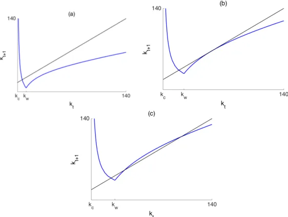
Taking into account Proposition 3.2, the Solow growth model with di↵erential saving and shifted Cobb-Douglas production function always admits the equilibrium k = 0 moreover multiple equilibria can exist: up to three positive fixed points are exhibited depending on the parameter values (see Figure 5). Note that the necessary condition for the existence of more then one positive equilibria is
sr< sw, moreover more than one positive fixed point can emerge for sufficiently high values of the
output elasticity of capital ↵. Note that these results agree with those obtained by Brianzoni et al. [19] considering the Revankar ([63]) VES production function: up to three positive fixed points may emerge if the elasticity of substitution is lower than one and workers save more than shareolders. Di↵erently, when a CES production function is considered, at most two positive fixed point may emerge (see Brianzoni et al. [14]).
Figure 5: Map and its positive fixed points for kt > kc in case of sr < sw for the following
parameter values: = 0.65, sw = 0.45, sr = 0.25, n = 0.45, A = 100, kc = 44. (a) One positive
fixed point for ↵ = 0.15, (b) two positive fixed points for ↵ = 0.275, (c) three positive fixed points for ↵ = 0.4.
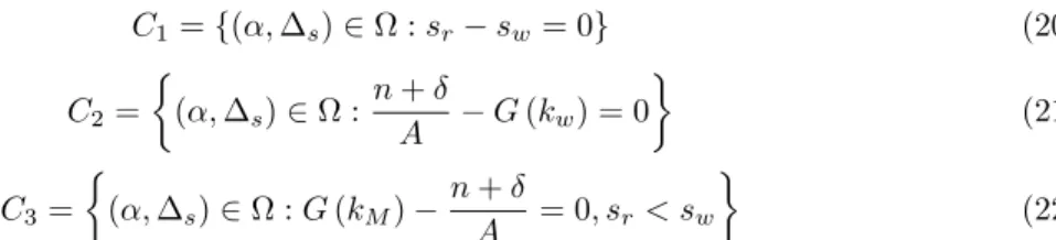
We want to highlight how the output elasticity of capital ↵ and the di↵erence between saving rates influence the number of steady states. For this purpose we define s= sr sw, s2 ( sw, 1 sw).
Taking into account the conditions related to the existence and number of fixed points stated in Proposition 3.2, it is possible to describe how the number of fixed points varies as the output elasticity of capital ↵ or the di↵erence between saving rates sis moved. To the scope we fix all
on the set ⌦ = [ sw, 1 sw]⇥ [0, 1]. Define C1={(↵, s)2 ⌦ : sr sw= 0} (20) C2= ⇢ (↵, s)2 ⌦ : n + A G (kw) = 0 (21) C3= ⇢ (↵, s)2 ⌦ : G (kM) n + A = 0, sr< sw (22)
then curves C1, C2and C3 separates the plane ⌦ into four regions: each region contains parameter
values corresponding to a case stated in Proposition 3.2.
Figure 6: Parameter values: = 0.05, sw = 0.4, n = 0.05, A = 3, kc = 20. Number of fixed
points according to Proposition 3.2. In blue region 1 positive fixed point (cases (i.b) and (ii.e)), in green region 1 positive fixed point (cases (i.a) and (ii.a)), in red region 3 positive fixed points (case (ii.c)). Curves C1, C2 and C3 are defined respectively in equations (20), (21) and (22).
The three regions are depicted in Figure 6: points on the right of C1 curve verify the condition of
the case (i) while the left region contain the parameter values related to the case (ii). The curve C2
verifies the condition (ii.d) while the curve C3verifies the condition (ii.b). Notice that the existence
of positive fixed points is due to high values of parameter ↵ combined with low values of parameter
s.
3.2.2 Stability of equilibrium levels
We now discuss about the local stability of the steady states of map . For what it concerns the local stability of the steady state k = 0, the following proposition holds.
Proposition 3.3. Let as given by (11). Then the equilibrium k = 0 is always locally stable. Proof. Note that limkt!0+ 0(kt) =
1
1+n2 [0, 1) and consequently the origin is a locally stable fixed
Notice that for all initial conditions k0 kc, map behaves as a contraction map and the iterations
monotonically converge to k = 0. Therefore we define the poverty trap as a situation in which, at the initial time, the capital per capita level is not high enough, i.e. k0 kc and such that in the
long term the economy will not survive. This result diverges from those obtained using a CES or VES production function (see Brianzoni et al. [14, 18, 19] and Grassetti et al. [29]) since a poverty trap exists (see also Capasso et al. [20] and Brianzoni et al. [16, 17]). Notice that CES and VES production functions well describe developed economies but are not able to capture the vicious circle of poverty that typically characterize non developed countries whereas the SCD production function allows to consider this phenomenon. Therefore, the presence of a poverty trap threaten the possibility of economic growth: economies starting from a low level of physical capital may be captured by the poverty trap and consequently the dynamic of physical capital will converge to zero. Note that for a small displacement from the stable equilibrium k = 0, the time trend of the relative displacement is Tr = (1+n1 )t. Therefore, if an economy lies in the poverty trap, an
higher depreciation rate of capital or an higher labour force growth rate causes a faster return to the steady state characterized by zero capital per-capita.
As the long term dynamics produced by the model are completely known for all initial capital per per worker less then the threshold value kc, we now focus on the growth patterns concerning
sufficiently high initial states (i.e. k0> kc).
For what it concerns the local stability of the positive hyperbolic steady state, the following propo-sition holds.
Proposition 3.4. Let as given by (11) and recall Proposition 3.2.
(i) Assume sr sw. If k⇤> kmin, the equilibrium k⇤ is locally stable. Otherwise 0(k⇤) < 0.
(ii) Assume sr< sw.
(a) Let g > G(kM). Then, if k⇤ > kmin the equilibrium k⇤ is locally stable. Otherwise 0(k⇤) < 0;
(b) Let G(kM) < g < G(kw) then the fixed point k3 > kM > kmin is always locally stable
while the fixed point kw > k2 > kM is always unstable. Furthermore if k1 > kmin, the
equilibrium k1 is always locally stable, whereas, if k1< kmin, then 0(k1) < 0;
(c) Let g < G(kw). Then the equilibrium k⇤ is locally stable.
Proof. Observe that 0(k) = 1 + A
1+nkG0(k). Being G0(k⇤) < 0 for cases (i), (ii.a) and (ii.e) of
Proposition 3.2, then 0(k⇤) = 1 + A
1+nk⇤G0(k⇤) < 1. Moreover is unimodal with minimum point
kmin, so that if k⇤ > kmin then 0(k⇤)2 (0, 1) whereas if k⇤ < kmin, 0(k⇤) < 0. In case (ii.c) k1
is stable if k1 > kmin while 0(k1) < 0 for k1< kmin. Moreover being G0(k2) > 0 then 0(k2) > 1
and consequently k3> k2> kmin is locally stable being (k) strictly increasing8k > kmin.
Notice that multiple equilibria coexist and hence multistability phenomena may occur. Therefore the global analysis of basins is mathematically significant (complex basins may exists) but especially economically relevant since it allow to answer one of the fundamental answers concerning developing countries and poverty trap: if an economy has a capital per capita level sufficiently high, i.e. k0> kc,
Further considerations on the nature of the fixed points, their basins and their behaviour are debated in the following section.
3.3
Complex attractors
In this section we analyze the qualitative asymptotic properties of map using both numerical simulations and analytical tools. Note that the map may show complex dynamics if a fixed point is located on the decreasing branch (see Proposition 3.4). In order to consider the possibility of complex attractors to emerge we analyze the case in which kmin > (kmin). Since the analytic
form of function is complicated, we cannot analytically describe this condition and the dynamic behaviour has to be analyzed by numerical simulations.
Recall from Proposition 3.4 that, if a fixed point is placed in the interval (kc, kmin) it may be locally
stable or unstable and hence a more complex attractor A may appear. The following proposition states the existence of a trapping interval for map .
Proposition 3.5. Let as given in (11). Assume kmin > (kmin) and, if three positive fixed
points exists, let k2> (kmin). Then the set J = [ (kmin), 2(kmin)] is trapping.
Being unimodal it admits a trapping set J under the conditions of Proposition 3.5, moreover as J is trapping then if a complex attractor A exists, it must belong to it. Furthermore A must attract the trajectory starting from the turning point kmin. Recall that if kmin > (kmin), then
the eigenvalue of the fixed point placed on the decreasing branch of map is negative and hence it may lose stability only via period-doubling bifurcation. Notice that subsequent bifurcations may be of the border collision type.
In Figure 7 we show three di↵erent staircase diagrams of map with initial condition k0= kminand
hence belonging to the trapping set J. In panel (a) a stable fixed point is presented for ↵ = 0.5. In panel (b) a stable cycle C2of period 2 is reached for ↵ = 0.4. Complexity emerges as the parameter
↵ decreases and a complex attractor is visible in panel (c) for ↵ = 0.35. In order to discuss the bifurcations leading to chaos within the trapping interval J defined in Proposition 3.5, we take in consideration the role of the di↵erence between saving propensities and the elasticity of substitu-tion. Figure 8 (a) contains the sequence of bifurcation of map as the parameter s is moved
while Figure 8 (b) shows the asymptotic dynamics versus the bifurcation parameter ↵.
In both the diagrams complex dynamics arise. Since f (kt) is a VES production function, we follow
the method presented in Chapter 1 in order to measure both the elasticity of substitution associ-ated to the attractor and the capital per-capita associassoci-ated to the attractor in order to analyze the relation between elasticity of substitution and capital per-capita equilibrium levels. As Figure 9 shows, an higher capital per-capita equilibrium level is linked to an higher elasticity of substitution, confirm the results obtained by Klump and La Grandville [42] considering the Solow growth model with a normalized CES production function. Figure 10 presents a cycle cartogram showing a two-parametric bifurcation diagram qualitatively: each color represents a long-run dynamic behaviour for a given initial condition in the parameter plane ( s, ↵). Cycles of di↵erent order are exhibited.
Notice that if ↵ is sufficiently small, then complex dynamics emerge if the di↵erence between work-ers and shareholdwork-ers is large enough. This result is in line with those obtained by Brianzoni et al.
Figure 7: Staircase diagram of being n = 0.3, = 0.6, sw = 0.25, sr = 0.5, A = 5, kc = 5 and
i.c. k0= kminfor di↵erent values of ↵. (a) ↵ = 0.5, stable fixed point. (b) ↵ = 0.4, stable 2-period
cycle. (c) ↵ = 0.35 complex attractor.
Figure 8: Parameter values n = sw = 0.3, = 0.2, A = kc = 1 and k0 = kmin. (a) Bifurcation