Leakages effect characterisation of an Iter cooling system through the development of a 1-d hydraulic model in OpenModelica

(1)

ALMA MATER STUDIORUM - UNIVERSITÀ DI BOLOGNA

SCUOLA DI INGEGNERIA E ARCHITETTURA

DIPARTIMENTO DI INGEGNERIA INDUSTRIALE

CORSO DI LAUREA MAGISTRALE IN INGEGNERIA ENERGETICA

TESI DI LAUREA

In

Metodi Numerici per l’Energetica M

LEAKAGES EFFECT CHARACTERISATION OF AN ITER COOLING

SYSTEM THROUGH THE DEVELOPMENT OF A 1-D HYDRAULIC

MODEL IN OPENMODELICA

Anno Accademico 2019/2020

Sessione III

CANDIDATO

RELATORE

Lorenzo Soverini

Chiar.mo Prof. Emanuele Ghedini

CORRELATORI

Ing. Benedetta Baldisserri

Davide Laghi

(2)

(3)

FIGURES

Figure 1.1 – EC Upper Launcher configuration ...14

(4)

Figure 1.2 – EC UL FCS assembly...15

Figure 1.3 – EC UL Waveguides Counter Flanges...16

Figure 1.4 – EC UL EVCS, Cooling System ...17

Figure 2.1 – OMEdit ...20

Figure 2.2 - Packages ...21

Figure 2.3 – OMPython test commands ...22

Figure 2.4 – Simulate Method ...22

Figure 2.5 – GetSolutions Method...22

Figure 2.6 – Extraction from a numpy array ...22

Figure 2.7 – getParameters Method ...23

Figure 2.8 – setParameters Method ...23

Figure 3.1 - EC UL EVCS, Layout ...25

Figure 3.2 – Data of the Nominal Hydraulic Model ...28

Figure 3.3 – Mass Flow Source ...29

Figure 3.4 – Mass Flow Source Parameters ...29

Figure 3.5 – Mass Flow Rate Meter ...30

Figure 3.6 - Pipe ...30

Figure 3.7 – Moody chart ...31

Figure 3.8 – Pipe Pressure Drop due to Friction ...32

Figure 3.9 – Pipe Parameters ...33

Figure 3.10 – Results for Pipes...34

Figure 3.11 – Orifice ...34

Figure 3.12 – Orifice Parameters ...35

Figure 3.13 – Results for Orifices...36

Figure 3.14 – Branch A ...37 Figure 3.15 – Branch B ...37 Figure 3.16 – Branch C ...38 Figure 3.17 – Branch D ...38 Figure 3.18 – Branch E ...39 Figure 3.19 – Branch F ...39

Figure 3.20 – Final Model ...41

Figure 4.1 – Badge Meter Preso® - Venturi Flow Meter ...43

Figure 4.2 – Badge Meter Preso® - Techincal Characteristics ...44

Figure 4.3 – ABB© - VTC – Venturi Tube ...44

(5)

Figure 4.7 – Obstruction Branch B ...46

Figure 4.8 – Obstruction Branch C ...47

Figure 4.9 – Obstruction Branch E1 ...47

Figure 4.12 – Obstruction Branch F ...49

Figure 4.13 – Class ...50

Figure 4.14 – Detection Branch A perturbed ...56

Figure 4.15 – Detection Branch B perturbed...56

Figure 4.16 – Detection Branch C perturbed...56

Figure 4.17 – Detection Branch E1 perturbed ...57

Figure 4.20 – Detection Branch F perturbed ...58

Figure 4.21 – Obstruction Branch B, plot ...62

Figure 4.22 – Obstruction Branch A, plot ...62

Figure 4.23 – Obstruction Branch E1, plot ...62

Figure 4.24 – Obstruction Branch C, plot ...62

Figure 4.27 – Obstruction Branch F, plot...63

Figure 5.1 – Branch A Leak start...67

Figure 5.2 – Branch A Leak middle ...67

Figure 5.3 – Branch A Leak end...68

Figure 5.4 – Branch B Leak start ...68

Figure 5.5 – Branch B Leak middle ...69

Figure 5.6 – Branch B Leak end ...69

Figure 5.7 – Branch C Leak start ...70

Figure 5.8 – Branch C Leak middle ...70

Figure 5.9 – Branch C Leak end ...71

Figure 5.10 – Branch E1 Leak start ...71

Figure 5.11 – Branch E1 Leak middle ...72

Figure 5.12 – Branch E1 Leak end ...72

Figure 5.13 – Branch E2 Leak start ...73

Figure 5.14 – Branch E2 Leak middle ...73

(6)

Figure 5.17 – Branch E3 Leak middle_1 ...75

Figure 5.18 – Branch E3 Leak middle_2 ...75

Figure 5.20 – Leakage Branch A start ...83

Figure 5.21 – Leakage Branch A middle ...85

Figure 5.22 – Leakage Branch B start...87

Figure 5.23 – Leakage Branch B middle ...89

Figure 5.24 – Leakage Branch C start...91

Figure 5.25 – Leakage Branch C middle ...93

Figure 5.26 – Leakage Branch E1 start ...95

Figure 5.27 – Leakage Branch E1 middle ...97

Figure 5.28 – Leakage Branch E2 start ...99

Figure 5.29 – Leakage Branch E2 middle ... 101

Figure 5.30 – Leakage Branch E3 start ... 103

Figure 5.31 – Leakage Branch E3 middle_1 ... 105

Figure 5.32 – Leakage Branch E3 middle_2 ... 107

Figure 5.33 – Detection Leakage Branch A start ... 108

Figure 5.34 – Detection Leakage Branch A middle ... 108

Figure 5.35 – Detection Leakage Branch B start ... 109

Figure 5.36 – Detection Leakage Branch B middle ... 109

Figure 5.37 – Detection Leakage Branch C start ... 109

Figure 5.38 – Detection Leakage Branch C middle ... 110

Figure 5.39 – Detection Leakage Branch E1 start ... 110

Figure 5.40 – Detection Leakage Branch E1 middle ... 110

Figure 5.42 – Detection Leakage Branch E2 middle ... 111

Figure 5.44 – Detection Leakage Branch E3 middle_1 ... 112

Figure 5.45 – Detection Leakage Branch E3 middle_2 ... 112

Figure 5.46 – Double Ended Guillotine Branch A start ... 113

Figure 5.47 – Double Ended Guillotine Branch A middle ... 113

Figure 5.48 – Double Ended Guillotine Branch A end ... 114

Figure 5.49 – Double Ended Guillotine Branch B start ... 114

Figure 5.50 – Double Ended Guillotine Branch B middle ... 115

(7)

Figure 5.54 – Double Ended Guillotine Branch C end ... 117

Figure 5.55 – Double Ended Guillotine Branch E1 start ... 117

Figure 5.56 – Double Ended Guillotine Branch E1 middle ... 118

Figure 5.57 – Double Ended Guillotine Branch E1 end ... 118

Figure 5.59 – Double Ended Guillotine Branch E2 middle ... 119

Figure 5.62 – Double Ended Guillotine Branch E3 middle_1 ... 121

Figure 5.63 – Double Ended Guillotine Branch E3 middle_2 ... 121

Figure 5.65 – Double Ended Guillotine Branch A start, Validation ... 125

Figure 5.66 – Double Ended Guillotine Branch A middle, outcomes ... 126

Figure 5.67 – Double Ended Guillotine Branch A end, outcomes ... 126

Figure 5.68 – Double Ended Guillotine Branch B start, outcomes ... 126

Figure 5.69 – Double Ended Guillotine Branch B middle, outcomes ... 127

Figure 5.70 – Double Ended Guillotine Branch B end, outcomes... 127

Figure 5.71 – Double Ended Guillotine Branch C start, outcomes ... 127

Figure 5.72 – Double Ended Guillotine Branch C middle, outcomes ... 128

Figure 5.73 – Double Ended Guillotine Branch C end, outcomes... 128

Figure 5.74 – Double Ended Guillotine Branch E1 start, outcomes ... 128

Figure 5.75 – Double Ended Guillotine Branch E1 middle, outcomes ... 129

Figure 5.76 – Double Ended Guillotine Branch E1 end, outcomes ... 129

Figure 5.78 – Double Ended Guillotine Branch E2 middle, outcomes ... 130

Figure 5.81 – Double Ended Guillotine Branch E3 middle_1, outcomes ... 131

Figure 5.82 – Double Ended Guillotine Branch E3 middle_2, outcomes ... 131

Figure 6.1 - Obstructions ... 133

Figure 6.2 – Small Breaks ... 134

TABLES

Table 3.1 – Cooling Data for EC UL EVCS ...26

(8)

Table 3.3 – Pressure Drop Data ...27

Table 3.4 – Orifices Data ...28

Table 3.5 – Branch Pressure Drop ...40

Table 3.6 – Branch Pressure Drop after the simulation ...40

Table 3.7 – Mass Flow Rates and pressure drops ...41

Table 3.8 – Mass Flow Rates and pressure drops after the simulation ...42

Table 4.1 – Minimum Mass Flow Rate...45

Table 4.2 – Minimum Mass Flow Rate in the model...49

Table 4.3 – Input Sensitivity ...59

Table 4.4 – Perturbed Pressure Drop and Perturbed Mass Flow Rates...59

Table 4.5 – Perturbed Pressure Drop and Perturbed Mass Flow Rates of the model ...60

Table 4.6 – Perturbed Pressure Drop and Perturbed Mass Flow Rates, Branch En_1 ...60

Table 4.7 – Perturbed Pressure Drop and Perturbed Mass Flow Rates of the model, Branch En_1 ...60

Table 4.9 – Perturbed Pressure Drop and Perturbed Mass Flow Rates of the model, Branch En_2 ...61

Table 4.11 – Perturbed Pressure Drop and Perturbed Mass Flow Rates of the model, Branch En_3...61

Table 4.12 – FM ΔMFR [%] ...64

Table 4.13 – FM ΔMFR [%] model...65

EQUATION

Equation 3.1 – Computation of the pressure drop in a pipe ...30

Equation 3.2 – Computation of the pressure drop in an orifice ...35

Equation 4.1 – Computation of Keq ...58

Equation 4.2 – Computation of K*_...58

Equation 4.3 – Computation of the pressure drop ...59

SCRIPT

Script 4.1 – Obstruction Branch A ...55

Script 5.1 – Leakage Branch A start ...80

(9)

(10)

Abstract

Il seguente elaborato è il risultato di 6 mesi di stage svolti presso NIER Ingegneria S.p.A. nell’ambito della modellazione idraulica dell’Ex-Vessel cooling system (EVCS) dell’Electron Cyclotron Upper Launcher (EC UL), un sottosistema di ITER (il reattore sperimentale a fusione nucleare in costruzione a Cadarache), tramite l’utilizzo del software OpenModelica. I temi trattati riguardano la modellazione del sistema in condizioni nominali e in condizioni di off-design (in presenza di ostruzioni o di rotture).

Per quanto riguarda il primo argomento, il sistema (in condizioni nominali) è stato modellato tramite OpenModelica, verificandone il design e appurando che le portate si distribuissero all’interno del sistema come desiderato.

Per quanto riguarda il secondo argomento, il sistema (in condizioni di off-design) è stato modellato in presenza di ostruzioni o di rotture. Nel caso di perdite di rotture sono stati considerati due scenari: piccole perdite e doppia ghigliottina. Per ciascun branch si sono considerate tre diversi posizioni della perdita: inizio, metà e fine del beam interessato dalla leak. Nel caso di piccole perdite si è considerato il beam collegato ad ambiente tramite una resistenza, mentre nel caso di doppia ghigliottina il beam era direttamente collegato ad ambiente. Per rendere più semplice il post-processing nello studio del sistema in condizioni di off-design è stato utilizzato OMPython. Gli obiettivi sono stati verificare che le variazioni di portata fossero rilevate dai misuratori di portata, presenti in mandata e ritorno di ogni branch. Inoltre, si è dovuto provare che la portata minima fosse garantita in ciascun componente per motivi di sicurezza. Tramite i vari modelli implementati con OpenModelica e simulati con OMPython si è potuto verificare che il design dell’EVCS soddisfa i requisiti definiti.

(11)

Abstract

The following dissertation is the result of a 6 months stage conducted at NIER Ingegneria S.p.A. in the hydraulic modelling of the Ex-Vessel cooling system (EVCS) of the Electron Cyclotron Upper Launcher (EC UL), a subsystem of ITER (the experimental fusion nuclear reactor under construction in Cadarache), through the use of the OpenModelica software. The topics discussed concern the modelling of the system in nominal operating conditions and in off-normal operating conditions (in presence of obstructions or leakage).

With regard to the first topic, the system (in nominal operating conditions) was modelled through the use of the OpenModelica software, proving the design and checking that the mass flow rates were distributed as desired within the system.

In off-normal operating conditions the system was modelled in presence of obstructions or leakage. In the case of leakages, two scenarios were considered: small breaks and double ended guillotine. Three different locations of the leak were assessed for each branch: start, middle and end of the beam affected by the leak.

In the case of small breaks, the beam was connected to ambient through a resistance, whereas in the case of double ended guillotine the beam was directly connected to ambient. OMPython was used to make the post-processing easier.

The objectives were to verify that flow rate variations could be detected by the mass flow rate meters, placed both in the feed and in the return of each branch. Moreover, it was needed to check that the minimum mass flow rate was provided in each component for safety purposes. Through various models implemented with OpenModelica and simulated with OMPython, it could be assessed that the EVCS design fulfils the defined requirements.

(12)

1 INTRODUCTION

This thesis is focused on the hydraulic modelling of the Ex-Vessel Cooling System (EVCS) of the Electron Cyclotron Upper Launcher (EC UL), a subsystem of ITER (the experimental fusion nuclear reactor under construction in Cadarache). The work was done at NIER Ingegneria S.p.A., a company that works in many sectors of engineering consulting, which is in charge of the EVCS design.

In the first part of the essay, the EC Upper Launcher configuration and its cooling system, and then the EC UL EVCS design and its layout (specifically on the main functions required) will be described. In the second part the hydraulic model of the EVCS in normal operating conditions will be presented, and its modelling through the use of the “OpenModelica” software [6] will be discussed.

After the analysis of the system in normal operating conditions, the hydraulic model in off-normal operating conditions will be introduced, such as the presence of obstructions or leakages. These studies are carried out by adopting OMPython [8], the OpenModelica Python Interface, implemented in Python; this software helped make the post-processing easier. Then the attention will be focused on the redistribution of flow rates through the various sections of the circuit and on the effects that these off-normal conditions can have on the cooling performance.

1.1 Objectives

The thesis is focused on the verification of two main requirements of the EVCS design:

the ability to provide a minimum mass flow rate to all the different actively cooled components it serves;

the ability to detect, through the use of mass flow meters, if the mass flow rate in one of the EVCS components decrease below its minimum.

The modelling of the system in nominal conditions was focused on the validation of the EVCS design, whose object is to provide the minimum mass flow rate in each component. The nominal model was implemented to assess that the pressure drop assigned to the orifice was adequate to achieve the desired distribution of flow rate in the system. In fact, given the design realised by NIER, given the total mass flow rate and the pressure budget available, the system was modelled by using OpenModelica and proving that the flow rates were actually redistributed through the various sections of the system as shown in Figure 3.2.

Regarding the system in off-normal conditions, the obstruction and the leakage were modelled with an orifice. A beam for every branch was perturbed each time by using the same input data of the nominal model. The aim was to find the pressure drop to assign to the orifice in order that the minimum mass flow rate was provided

(13)

value in a component. Two different leakages scenario were evaluated: small break and double ended guillotine. Three different locations were considered for each leak: start, middle and end of the beam. The objectives for small breaks were to find which was the pressure drop to assign to the orifice that provided the minimum mass flow rate in the component following the leak and if the mass flow rate meters (placed both in the feed and in the return of each branch) could detect mass flow rate variations. As regards double ended guillotine, it was analysed how the flow rates were distributed within the system and where a flow reversal occurred.

1.2 Electron Cyclotron Upper Launcher

This chapter provides the description of the Electron Cyclotron Upper Launcher, its configuration and its cooling system.

1.2.1 Electron Cyclotron Heating and Current Drive

ECH&CD provides 170 GHz high power microwave beams for plasma heating and current drive applications. ECH&CD consists of four main subsystems: high voltage power supply (HVPS), radio frequency source (RF), transmission line (TL) and launchers.

ECH&CD includes two types of launchers that transfer power to the plasma:

a launcher is located in the equatorial port (Equatorial Launcher, EL), used for concentrated storage of power, and has the function of decoupling heat from the current driving function;

four launchers are located in the four upper ports (Upper Launchers, UL), used to deposit power in the outer half of the plasma cross-section to control magnetohydrodynamic instabilities.

1.2.2 Cooling System Configuration

As shown in Figure 1.1, the composition of each EC Upper Launcher is as follows:

the "First Confinement System" (FCS), which is the assembly of components extending the first confinement barrier of the Vacuum Vessel volume, installed “ex-Vessel” (i.e. in the port cell and interspace)

the "Upper Launcher" which is the assembly of structural, optical and shielding components, installed “in-Vessel” (i.e. within the Vacuum Vessel boundary)

(14)

Figure 1.1 – EC Upper Launcher configuration

1.2.3 Configuration

The EC Upper Launcher cooling system consists of two independent distribution systems:

The EC UL Ex-Vessel cooling system can provide fresh water to the EC FCS components;

The EC UL In-vessel cooling system can provide fresh water and gas (nitrogen for maintenance) to the EC UL components.

The EC UL Ex-Vessel and In-Vessel cooling system must meet different requirements, due to the different components to be cooled, functions required and environmental and loading conditions experienced during operations, testing and maintenance, incidents and accidents. The design of the EC UL EVCS is clearly related to the design of the EC UL FCS. Figure 1.2 and Figure 1.3 show the different components of the EC UL FCS that are cooled by the EVCS:

Thermal Insulation - Closure Plate Sub Plate (TI-CPSP); Waveguides in Port Cell, in Interspace (WGs-PC, WGs-IS);

Waveguide Counter Flanges in Port Cell, in Interspace (WGs CF-PC, WGs CF-IS); Mono Block Mitre Bend body (MBMB-b) and mirror (MBMB-m);

Mitre Bend body (MB-b) and mirror (MB-m); Isolation Valve (IV);

Diamond Window Unit (DWU).

(15)

The DWU includes a (~1.1 mm thick) disk made by low RF power loss and higher thermal conductivity material. Cooper cuffs with relatively thin copper walls (~1 mm) are brazed to the diamond disk and can be indirectly cooled. The IV is an all-metal valve which must be closed to advance the first confinement system from the DWU, in the event of vacuum volume overpressure (i.e. in the event of coolant leakage).

The ex-vessel WGs and optical components (MB and MBMB) are connected (from the CPSP up to the IV) through flange couplings with Double Metal Seal (DMS) and online leak monitoring of the seals interspace.

(16)

Figure 1.3 – EC UL Waveguides Counter Flanges

1.2.4 Electron Cyclotron Upper Launcher Ex-Vessel Cooling System

1.2.4.1 Main Function

The main functions required to the EC UL EVCS are to:

provide water to and retrieve it from the EC UL Ex-Vessel (and TL) components internal cooling in order to make possible the heat removal from the EC UL Ex-Vessel (and TL) components (subjected to thermal power due to ohmic losses during mm-wave propagation);

(17)

It requires the capability of the system:

to balance the pressure drops through FCS components; to regulate the coolant flows through FCS components;

to isolate the circuit in case of failure and for maintenance purposes; to monitor the coolant parameters and specifically;

to detect loss of cooling condition to protect FCS components;

to interface with the internal cooling circuits of the FCS cooled components;

to interface with the Port Cell and Interspace building, with the penetration in the Bio-Shield that delimits them, with the CCWS-1, with the Cable Trays (for the sensors) and with the Gallery TL and Shutter Valve; to ensure the required structural stiffness and mechanical stability against dynamic loads acting on the launcher during ITER operations (e.g. forces and moments due to plasma disruptions) and external events (e.g. seismic);

to allow and facilitate manual assembly, welding, screwing and inspection.

1.2.5 Location

According to the physical location of the components, two parts of EC UL EVCS are defined, as shown in Figure 1.4:

PCC (Port Cell Components) including all components hosted in the Port Cell;

ISC-CCWS (InterSpace Components belonging to CCWS) including all components in the Interspace.

(18)

1.2.6 Technical Solution

1.2.6.1 Instrumentation for Monitoring

The system is equipped with the instrumentation (measurement sensors) required to:

monitor coolant temperature to facilitate fault localization by coolant temperature measurements;

monitor coolant pressure at the inlet line by coolant pressure and differential pressure measurements; detect coolant losses by flow measurements;

detect flow obstructions by flow measurements.

Temperature measurements have been set to provide data as follows: Inlet temperature – upstream of inlet manifold;

Component outlet temperatures – downstream of component or group of components; Mixing temperatures – downstream of coolant mixing points ;

Outlet temperature – downstream of outlet manifold .

Pressure gauge sensors have to be installed at the inlet of the circuit.

Differential pressure sensors have to be installed between inlet and outlet of the circuit.

Flow measurement devices have to be installed at the inlet and outlet of branches A1, A2, B1, B2, C1, C2, E1, E2, E3, E4, E5, E6, E7, E8 and F.

The focus in this thesis was to assess the detection of flow in case of obstruction or leakage.

1.3 Abbreviations

The general list of ITER acronyms used for the present document is reported below. CCWS Component Cooling Water System

DMS Double Metal Seal DN Nominal Diameter DWU Diamond Window Unit EC Electron Cyclotron

EV Ex-Vessel

EVCS Ex-Vessel Cooling System FCS First Confinement System

(19)

MB Mitre Bend

MBMB Mitre Bend MonoBlock MFR Mass Flow Rate

PC Port cell

TI-CPSP Thermal Isolation Closure Plate SubPlate TL Transmission Lines

UL Upper Launcher

WG WaveGuide

WGCF WaveGuide Counter Flange

2 METHODOLOGY

Tools and software used are presented below. OpenModelica was adopted for creating models, by using components within the Fluid section. OMPython was used for simulating models, because it made the post-processing easier, and for creating iterative cycle for finding the pressure drop that provided the minimum mass flow rate in the component affected by the obstruction or the leakage.

2.1 OpenModelica

OpenModelica is an open source Modelica-based modelling and simulation environment intended for industrial and academic usage; in particular, it was used OMEdit [7], an open-source graphical interface for creating, editing and simulating Modelica models in textual and graphical modes. OMEdit communicates with OMC through an interactive API, requesting model information and creating models/connection diagrams based on the Modelica annotations.

(20)

Figure 2.1 – OMEdit

The section dedicated to Fluid within the Modelica environment was specifically used. Among the packages listed in Figure 2.2, were used:

Pipes Fittings Sources Sensors

The components were selected from respective packages and then dragged to the modelling ambient, in order to add them in the model. Every time a component was added in the model, it was registered in the text view with its parameters.

(21)

The compilation of the model required that the fluid that flowed in each element was specifically defined. The Ex-Vessel Cooling System is fully crossed by water. There were a lot of packages for the definition of the carrier fluid: air, compressible and incompressible fluids, ideal gas and R134a. A specific one was created, called ‘MyWater’, starting from the ‘ConstantPropertyLiquidWater’ package available on OpenModelica: by using this package, the density, specific heat capacity (at constant pressure and constant volume) and the dynamic viscosity could be set as constants (equal to the values in the hydraulic model, respectively 994.752 [kg/m3_{], 4176.904 [J/Kg K] and 0.000734 [Pa s]). The following expression must be used in the text view for} each component: redeclare package Medium = MyWater.

2.2 OMPython

OMPython is the OpenModelica Python Interface implemented in Python. It is a free, open source, highly portable Python based interactive session handler for Modelica scripting. It provides the modeler with the components needed to create a complete Modelica modelling, compilation and simulation environment and it is designed to combine both the solving strategy and model building. The obstruction and the leakage model were simulated through OMPython. It was used Jupyter notebook, an open-source web application, and Spyder, a free and open-source scientific environment written in Python, to creating the script.

2.2.1 Test Commands

First, the OMPython library was imported from Python. OMPython provides two classes of communication with OpenModelica: OMCSession and OMCSessionZMQ. Both classes had the same interface and the OMCSessionZMQ was used, because it is recommended on the OpenModelica website [6]. An

(22)

OMCSessionZMQ object was created to test the command outputs by importing it from the OMPython library within Python interpreter. This module allowed to interactively send commands to the OpenModelica server and display their output. A Modelica System object was then introduced; the object constructor requires a minimum of 2 input arguments which are strings:

The first input argument must be a string with the file name of the Modelica code, with Modelica file extension ‘.mo’. if the Modelica file is not in the current directory of Python, then the file path must also be included.

The second input argument must be a string with the name of the Modelica model.

Figure 2.3 – OMPython test commands

The ‘simulate’ method was then adopted, which simulates model according to the simulation options:

Figure 2.4 – Simulate Method

The data for the post-processing had to be obtained, by using this procedure:

Figure 2.5 – GetSolutions Method

‘Data_File_name’ represents the name of the component in the model, depending on whether the mass flow rate or the pressure of the component was needed and indicated if it concerned the input or the output. The getSolutions method returns a list of numpy arrays. It can be called with a list of quantities name (or a single quantity name) in string format as argument; it returns the simulation results of the corresponding names in the same order.

One element from the numpy array must be extracted, through the following statement:

(23)

Figure 2.7 – getParameters Method

The argument is the parameter’s name used in the OpenModelica model, and it returns the corresponding parameter value. In this way it could be checked if the variable was equal to the one applied in the model.

Figure 2.8 – setParameters Method

This is used to set parameters values. It can be called with a sequence of parameter name and assigning corresponding value as argument. For example, the pressure drop or the nominal mass flow rate of a component could be changed and start a new simulation.

The Mass Flow Rate Meters have been neglected in the following simulations implemented through OMPython because they would have been useful only if there had been a feedback control on the mass flow rate within the system.

(24)

3 HYDRAULIC MODELLING OF EC UL EVCS

3.1 System Layout

A representative diagram is provided in Figure 3.1.

Each Launcher cooling circuit has been divided in six branches arranged in parallel, namely:

Branch A serving the TL components in the Port Cell including the Isolation Shutter Valve (ISV) and the WGs in Port Cell.

Branch B serving the WGCF in Port Cell. Branch C serving the DWUs and the IVs.

Branch D dedicated to the TL components in the Gallery.

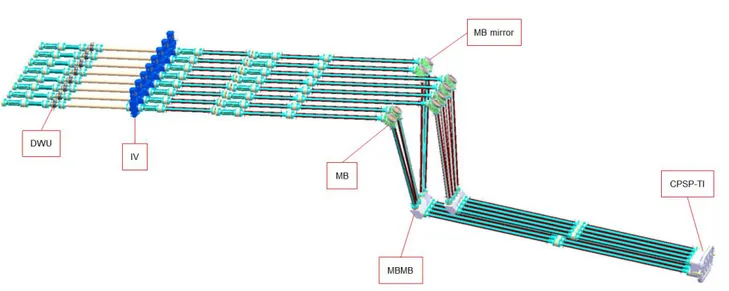
Branch E serving the components in the Interspace, i.e. MBMB Mirror and Body, MB Mirror and Body, WGs and their WGCFs.

Branch F dedicated to the TI-CPSP in the Interspace.

The 6 branches are connected to the CCWS-1A through a couple of manifolds (supply and return).

The branches A, B and C have the same layout: the main branch splits in two sub-branches, each connected to a manifold which distributes the flow among 4 Lines, one per beam. The flow is collected downstream by 2 manifolds, one per each sub-branch, prior to join again in the branch return line.

The branch D, for the purpose of the present activity, is treated as a black box, provided that the required mass flow rate is supplied by the EVCS.

The branch E, dedicated to the components in the Interspace, is the only one adopting a “per-beam” structure. The branch supply is connected to a manifold which distributes the flow among 8 sub-branches, one per beam. Each sub-branch is then directed towards a manifold, which distributes the flow among 3 lines based on the components to be cooled as follows:

Line En1 serving the WGCFs.

Line En2 serving the MBMB Mirror and the MB Mirror. Line En3 serving the MBMB Body, the MB Body and the WGs.

Downstream the components, a two-stage manifold similar to the supply layout is used, so the flow can be recollected.

Branch F directs the flow directly through the TI-CPSP.

For branches E and F, valves, sensors and orifices have been placed outside the bioshield (i.e. in the Port Cell), to ensure higher radiation protection and better accessibility for maintenance during the nuclear phase.

(25)

Figure 3.1 - EC UL EVCS, Layout

3.2 Cooling Data for EVCS Circuit

Each of the EVCS circuits is provided with appropriate coolant mass flowrate to remove the thermal load of the components it cools while keeping the outlet temperature within prescribed limits. In Table 3.1 the mass flow rate into each cooling line, branch and sub-branch is defined.

Cooling Section Component MFR MFR MFR

Branch Sub-Branch

Line ID [kg/s] [kg/s] [kg/s]

A A1 A1n (x4) TL-PC, ISV, WG-PC 0.297 1.188 2.376

(26)

B B1 B1n (x4) WGF-PC 0.023 0.092 0.184 B2 B2n (x4) WGF-PC 0.023 0.092 C C1 C1n (x4) DWU, IV 0.106 0.424 0.848 C2 C2n (x4) DWU, IV 0.106 0.424 D - - TL-G - - 2.376 E En (x8) En1 WGF-IS 0.030 0.426 3.408 En2 MBMB-m, MB-m 0.106 En3 WG-IS, MBMB-b, MB-b 0.290 F - - TI-CPSP - - 0.233

Table 3.1 – Cooling Data for EC UL EVCS

PIPING

NAME MFR [Kg/s] L [m] DN D [m] v [m/s]

Inlet-Outlet 9.425 20.6 65 6.69E-02 2.69540743

Branch A 2.376 2 25 2.79E-02 3.90690928

Branch A-1 1.188 30.7 25 2.79E-02 1.95345464

Branch A-2 1.188 30.7 25 2.79E-02 1.95345464

Branch B 0.184 2 15 1.71E-02 0.8054172 Branch B-1 0.092 27.2 15 1.71E-02 0.4027086 Branch B-2 0.092 27.2 15 1.71E-02 0.4027086 Branch C 0.848 2 20 2.25E-02 2.14400658 Branch C-1 0.424 28.2 20 2.25E-02 1.07200329 Branch C-2 0.424 28.2 20 2.25E-02 1.07200329 Branch E 3.408 2 50 5.48E-02 1.45255895

Branch E-0 0.426 28.5 15 1.71E-02 1.86471591

Branch E-1 0.03 12.8 10 1.38E-02 0.2016315

Branch E-2 0.106 12.8 10 1.38E-02 0.7124313

Branch E-3 0.29 12.8 10 1.38E-02 1.94910449

Branch D 2.376 2 32 3.67E-02 2.25792549

Branch F 0.233 54.6 15 1.71E-02 1.0199033

Table 3.2 – Pipes Data

COMPONENTS PRESSURE DROP

(27)

Waveguides in Port Cell A-1 WG-PC 3.13E+04

Waveguides Flanges in Port Cell B-1 WGF-PC 1.20E+05

Diamond Window Unit C-1 DWU 5.70E+03

Isolation Valve C-1 IV 1.60E+04

Transmission Lines in PC + Shutting Valves A-2 TL-PC+ISV 6.29E+04

Waveguides in Port Cell A-2 WG-PC 3.13E+04

Waveguides Flanges in Port Cell B-2 WGF-PC 1.20E+05

Diamond Window Unit C-2 DWU 5.70E+03

Isolation Valve C-2 IV 1.60E+04

DMS Miter Bend Mirror E-2 MB-m 1.50E+04

DMS Miter Bend Body E-3 MB-b 1.93E+04

DMS Mono Block Miter Bend Mirror (each) E-2 MBMB-m 1.50E+04

DMS Mono Block Miter Bend Body (each) E-3 MBMB-b 1.93E+04

Waveguides in Interspace E-3 WG-IS 3.28E+04

Waveguides Flanges in Interspace E-1 WGF-IS 9.53E+04

Thermal Isolation Closure Plate SubPlate F TI-CPSP 6.00E+04

Flowmeter A-1 A-1 FM 1.00E+05

Flowmeter A-2 A-2 FM 1.00E+05

Flowmeter B-1 B-1 FM 1.00E+05

Flowmeter B-2 B-2 FM 1.00E+05

Flowmeter C-1 C-1 FM 1.00E+05

Flowmeter C-2 C-2 FM 1.00E+05

Flowmeter E-0 E-0 FM 1.00E+05

Flowmeter F F FM 1.00E+05

Table 3.3 – Pressure Drop Data

ORIFICES LINE ΔP [Pa] Branch A 207832.7512042193 Branch B 284221.3997869775 Branch C 357707.11236831703 Branch D 394832.67754760385 Sub-Branch E1 239270.17538552155 Sub-Branch E2 297951.92807152064 Sub-Branch E3 216606.1702615875

(28)

Figure 3.2 – Data of the Nominal Hydraulic Model

The model was realized in the form of a MS Excel spreadsheet by NIER, through which the hydraulic model of the EC UL EVCS was implemented, and consisted of the following 7 sections:

1. Definition of reference input data. 2. Pressure losses from CFD analysis. 3. Piping data.

4. Characterization of combined pressure losses.

5. Derivation of Equivalent Pressure Loss Coefficients (EPLCs). 6. Summary of Orifices and Valves.

Branch F 303852.04572093795

Inlet-Outlet 20084.0

(29)

The data reported in the previous Figures and Tables was accessible in an Excel file [3] which has been made available for the modelling of the system through OpenModelica.

3.3 Components

- Mass Flow Source

It represented the main source of the system. Only one parameter could be set, the mass flow rate, which is equal to 9.425 kg/s, as shown in Table 3.2 (inlet-outlet).

Figure 3.4 – Mass Flow Source Parameters Figure 3.3 – Mass Flow Source

(30)

- Mass Flow Rate Meter

Mass Flow Rate Meters were used to verify the correct repartition of flow within the system. The modelled system through OpenModelica has validated the location of the Mass Flow Rate meter; instead of locating a mass flow rate meter in each beam (configuration not acceptable for lack of space), it was placed upstream and downstream of the beam, proving the correct distribution of flow.

- Pipe

Pipes were used to define the length of the different branches and of the piping in the beam. The parameters that had to be set were length and diameter, which are shown in Table 3.2. Starting from these parameters, the software evaluated fluid’s pressure at inlet (port_a) and at outlet (port_b) of pipes.

For pipes with circular cross section the pressure drop is computed as [9]: 𝑑𝑝 = λ(Re, D) ∙ (L D) ∙ ρ ∙ v ∙ |v| 2 = λ(Re, D) ∙ 8 ∙ L π2_{∙ D}5_{∙ ρ}∙ mflow ∙ |mflow|

= λ2(Re, D) ∙ k2∙ sign(mflow);

Equation 3.1 – Computation of the pressure drop in a pipe

with

𝑅𝑒 = |v| ∙ D ∙ ρ/μ = m_flow| ∙ 4/(π ∙ D ∙ μ)

𝑚𝑓𝑙𝑜𝑤 = 𝐴 ∙ 𝑣 ∙ ρ

Figure 3.5 – Mass Flow Rate Meter

(31)

𝑘2= 𝐿 ∙ 𝜇2/(2 ∙ 𝐷3∙ 𝜌)

where:

L is the length of the pipe.

D is the diameter of the pipe. If the pipe has not a circular cross section, 𝐷 = 4 ∙ 𝐴/𝑃, where A is the cross section area and P is the wetted perimeter.

𝜆 = 𝜆(𝑅𝑒, 𝐷) is the "usual" wall friction coefficient.

𝜆 2= 𝜆 ∙ 𝑅𝑒2 is the used friction coefficient to get a numerically well-posed formulation.

𝑅𝑒 = |𝑣| ∙ 𝐷 ∙ 𝜌/𝜇 is the Reynolds number.

D = d/D is the relative roughness where "d" is the absolute "roughness", i.e., the averaged height of asperities in the pipe (d may change over time due to growth of surface asperities during service). ρ is the upstream density.

μ is the upstream dynamic viscosity. v is the mean velocity.

The first form with λ is used:

(32)

This form is not suited for a simulation program since λ = 64/Re if Re < 2000, i.e., a division by zero occurs for zero mass flow rate because Re = 0 in this case. More useful for a simulation model is the friction coefficient 𝜆 2= 𝜆 ∙ 𝑅𝑒2, because 𝜆 2= 64 ∙ 𝑅𝑒 if Re < 2000 and therefore no problems for zero mass flow rate occur.

The characteristic of λ2 is shown in the next figure and is used in Modelica.Fluid:

Figure 3.8 – Pipe Pressure Drop due to Friction

In the system we have Re ≥ 4000 so the flow is turbulent, and the following statement is used to evaluate the pressure drop in pipes:

if the pressure drop dp is assumed to be known, 𝜆₂ = |𝑑𝑝|/𝑘2. The Colebrook-White equation:

1/√𝜆 = −2 ∙ log10(2.51/(𝑅𝑒 ∙ √𝜆) + 0.27 ∙ 𝐷)

gives an implicit relationship between Re and λ. Inserting 𝜆 ₂ = 𝜆 ∗ 𝑅𝑒2 allows to solve this equation analytically for Re:

(33)

If the mass flow rate is assumed known (and therefore implicitly also the Reynolds number), then λ2 is computed by an approximation of the inverse of the Colebrook-White equation adapted to λ2:

𝜆2 = 0.25 ∙ (𝑅𝑒/log10(𝐷/3.7 + 5.74/𝑅𝑒0.9))2

The pressure drop is then computed as 𝑑𝑝 = 𝑘₂∙ 𝜆2∙ 𝑠𝑖𝑔𝑛(𝑚_𝑓𝑙𝑜𝑤).

A pipe was added for each beam, with length equal to 12.8 m and diameter equal to 13.8e-3_{m. The value} proposed by OpenModelica for the roughness (2.5e-5_{m) was adopted.}

Two pipes for the modelling of branches (A, B, C, E, F) and sub-branches (An, Bn, Cn, E0) were used, to which

I assigned a length equal to the half of the length shown in Table 3.2. For example, Branch A has a length of 2 m, so two pipes of 1 m each were used.

Figure 3.9 – Pipe Parameters

After the simulation it was possible to:

verify if the flow crossed the pipe correctly, checking that the mass flow rate in port_a was equal to the one in port_b.

calculate the pressure drop in the pipe, as the difference between the pressure in port_a, and the one in port_b.

(34)

Figure 3.10 – Results for Pipes

- Orifices

Orifices were used a) to model the components present in the system and b) as real orifices, because of their presence in each branch (as shown in Table 3.2). Regarding the components’ modelling, given their pressure drop (as reported in Table 3.3), 1) a nominal flow equal to the one that crossed a particular component in a specific branch and 2) a nominal pressure drop equal to the one indicated in Table 3.3 were assigned to the orifice.

(35)

Figure 3.12 – Orifice Parameters

In general, depending on the location of the component, the mass flow of the branch or of the beam was used as m_flow_nominal (Table 3.2), and the pressure drop of the component (Table 3.3) as dp_nominal. Each time there was more than one component in a branch, a single orifice was added in the model with a nominal pressure drop equal to the sum of the pressure drops of the components. An orifice was adopted for the modelling of the pressure drop linked with the Mass Flow Rate meters of each sub-branch, giving a nominal loss equal to the half of the value represented in Table 3.3. Moreover, the values of the pressure drop shown in Table 3.4 were used for the modelling of the orifices.

For the evaluation of the orifice’s pressure drop a generic diameter must be set, whereas the coefficient zeta was computed by the software from dp_nominal and m_flow_nominal; OpenModelica used the following equation for the estimation of the pressure drop in an orifice [10]:

𝑑𝑝 = 0.5 ∙ 𝑧𝑒𝑡𝑎 ∙ 𝜌 ∙ 𝑣 ∙ |𝑣| = 0.5 ∙ 𝑧𝑒𝑡𝑎 ∙ 𝜌 ∙ 1/(𝑑 ∙ 𝐴)2_{∙ 𝑚_𝑓𝑙𝑜𝑤 ∙ |𝑚_𝑓𝑙𝑜𝑤|} = 0.5 ∙ 𝑧𝑒𝑡𝑎/𝐴 2∙ 1/𝜌 ∙ 𝑚_𝑓𝑙𝑜𝑤 ∙ |𝑚_𝑓𝑙𝑜𝑤| = 𝑘/𝜌 ∙ 𝑚_𝑓𝑙𝑜𝑤 ∙ |𝑚_𝑓𝑙𝑜𝑤| 𝑘 = 0.5 ∙ 𝑧𝑒𝑡𝑎/𝐴2 = 0.5 ∙ 𝑧𝑒𝑡𝑎/(𝑝𝑖 ∙ (𝐷/2)2)2 = 8 ∙ 𝑧𝑒𝑡𝑎/(𝑝𝑖 ∙ 𝐷2₎2

Equation 3.2 – Computation of the pressure drop in an orifice where:

Δp is the pressure drop: 𝛥𝑝 = 𝑝𝑜𝑟𝑡_𝑎. 𝑝 − 𝑝𝑜𝑟𝑡_𝑏. 𝑝

D is the diameter of the orifice at the position where ζ is defined (either at port_a or port_b). If the orifice has not a circular cross section, 𝐷 = 4 ∙ 𝐴/𝑃, where A is the cross-section area and P is the wetted perimeter.

(36)

ζ is the loss factor with respect to D that depends on the geometry of the orifice. In the turbulent flow regime, it is assumed that ζ is constant.

For small mass flow rates, the flow is laminar and is approximated by a polynomial that has a finite derivative for m_flow=0.

v is the mean velocity. ρ is the upstream density.

As for pipes, it was possible to verify if the flow crossed the orifice correctly and to evaluate the pressure drop in the orifice.

Figure 3.13 – Results for Orifices

Before starting the simulation, it must be checked if the number of variables was equal to the number of equations: this assessment was necessary in order to verify that each parameter was defined and that each component was properly collected.

(37)

3.4 Modelling of Branches

Before implementing the final model, each branch was designed separately, by using the pressure drop of the components as input data, and by checking among output data, in nominal conditions, that flows were distributed in a similar way (if not identical) to the desired ones.

Branch A

For the modelling of Branch A, a Mass Flow Source was adopted, setting the flow equal to the value of the nominal one for the branch (2.376 kg/s). Branch A (as every other branch) ended with a Boundary, with ambient temperature and pressure. The same operations were repeated for Branch B and C, changing pipes’ length, nominal flow of the branch and pressure drop linked with the orifice. The pipes circled in red represent the length of the branch, whereas the ones circled in yellow represent the length of the beam.

Figure 3.14 – Branch A

Branch B

(38)

Branch C

Figure 3.16 – Branch C

Branch D

Branch D was considered like a black-box and was modelled with a single orifice, with a nominal pressure drop equal to the one of the TL-G component.

(39)

Branch E

Figure 3.18 – Branch E

In the sub-branches En two orifices were added, one to model the component and one to model the orifice.

Branch F

(40)

3.5 Implementation of the Model

Once all the data were added and after properly collecting all the components, it was possible to start the simulation. It was checked that, among output data, the pressure drops of the branches were equal to the value in Table 3.5, which represented the maximum pressure drop that the EVCS could have: these values represented the pressure drops each branch could have, considering that the different branches were in parallel.

Table 3.5 – Branch Pressure Drop

Then the final model was built, creating a new one in which the models of each branch previously computed were copied. LINE ΔP [Pa] Branch A 5,10E+05 Branch B 5,10E+05 Branch C 5,10E+05 Branch D 5,10E+05 Branch E 5,10E+05 Branch F 5,10E+05 LINE ΔP [Pa] Branch A 5,1011406665968394E+05 Branch B 5,100022205811641E+05 Branch C 5,101266252591538E+05 Branch E 5,1011420132277475E+05 Branch F 5,1012510391823796E+05

(41)

Figure 3.20 – Final Model

Inlet and outlet pipes were added in the final model: both with a length equal to the half of the value reported in Table 3.2. An orifice was also added, linked to the inlet-outlet line,with a pressure drop equal to the one in Table 3.4. Then it was evaluated that flows were correctly distributed among sub-branches, branches and beams, also monitoring that the pressure drops in them were comparable with the desired values represented in the following Table:

LINE MFR [kg/s] ΔP [Pa]

En_1 0,03 3,35E+05

En_2 0,106 3,35E+05

En_3 0,29 3,35E+05

Branch An losses 1,188 1,47E+05

Branch Bn losses 0,092 1,04E+05

Branch Cn losses 0,424 1,19E+05

N-th Beam An 0,297 1,44E+05

N-th Beam Bn 0,023 1,21E+05

N-th Beam Cn 0,106 2,91E+04

Table 3.7 – Mass Flow Rates and pressure drops

LINE MFR [kg/s] ΔP [Pa]

En_1 0,02999928192152918 3,353400358991654 E+05

En_2 0,1059961625000304 3,353400358991654 E+05

(42)

Branch An losses 1,187964657359805 1,47088.66322448244 E+05

Branch Bn losses 0,09200747951639193 1,0432142446628353 E+05

Branch Cn losses 0,4239826544980565 1,1851540502448194 E+05

N-th Beam An 0,29699116433995125 1,4371174865476944E+05

N-th Beam Bn 0,0230018698790979825 1,2039538880781742 E+05

N-th Beam Cn 0,105995663624514125 2,910994252950151 E+04

(43)

4 HYDRAULIC MODELLING OF EC UL EVCS

WITH OBSTRUCTIONS

After the analysis of the system in nominal operating conditions, the study of the system in off-normal operating conditions was carried out, particularly in presence of obstructions. The aim was to check if the instrumentation system of the EC UL EVCS was able to detect, in case of an obstruction, if the mass flow rate in a certain component dropped below the minimum required value (which had to be higher than the uncertainty of the instrument). Each component has a minimum mass flow rate for safety purposes: this obviously resulted in a minimum mass flow rate for each branch.

4.1 Venturi Flowmeters

The flowmeters adopted in the EC UL EVCS design for detecting loss of cooling water were Venturi tubes. Venturi flowmeter belongs to the differential pressure devices family and “consists of a convergent inlet connected to a cylindrical throat which is in turn connected to a conical expanding section calling the divergent”. Measuring the differential pressure Δp between the upstream section and the throat section, the volumetric flow rate q can be determined, given the value of the discharge coefficient C, depending on Venturi tube dimensions and manufacturing. The mass flow rate ṁ calculation needs the conditions of the fluid at the inlet of the tube in terms of pressure p1 and temperature T1, in order to know the fluid density ρ1.

The application requires Venturi tubes inserted in line having nominal size between DN15 and DN25. Such flow elements are provided with calibrated accuracy on the discharge coefficient between 0.25% and 0.5%. The accuracy from 0.5 to 0.63 was reached by considering that Venturi flowmeters measure volumetric flow rates which then need to be transformed in mass flow rates. At this point the inaccuracies due to pressure and temperature measurement must be considered. The accuracy of the device was set equal to 0.63%. Some devices present on the market are reported below with their technical characteristics:

BADGE METER – PRESO® - Venturi Flow Meter

(44)

Figure 4.2 – Badge Meter Preso® - Techincal Characteristics

ABB© – VTC - Venturi Tube

Figure 4.3 – ABB© - VTC – Venturi Tube

Figure 4.4 – ABB© - VTC – Technical Characteristics

The accuracy of the instruments is ± 0.5% in both cases, with an accuracy of the Venturi adopted in the system of 0.63%, comparable with the values obtained in the model, as indicated in Table 4.13.

(45)

4.2 Obstructions Modelling

Mass flow sources and boundaries used in the previous simulation were replaced with two boundaries with prescribed pressure: one was placed at the input of the system, with a pressure of 9.5 bar and one was placed at the output of the system, with a pressure of 4 bar. In this way the model could be implemented working with a prescribed pressure drop for the system (equal to 5.5 bar, as shown in Figure 3.2), with mass flow rates redistributing through the various sections of the system (depending on where the obstruction was located). An orifice was placed in each branch to model the obstruction within the system (as shown in the following Figures) with a pressure drop so that the minimum cooling mass flow rate was provided in the perturbed branch. LINE MFRMIN En_1 0,02 En_2 0,087 En_3 0,27 N-th Beam A 0,27 N-th Beam B 0,02 N-th Beam C 0,087 Branch F 0,2

Table 4.1 – Minimum Mass Flow Rate

Each branch was extended time by time to simplify the system, after checking the proper value of the pressure drop and of the mass flow rates of the total model. The other branches were modelled with an orifice, to which it was assigned a pressure drop equal to the one indicated in Table 3.5: this caused a small variation to the nominal mass flow rates of the system.

(46)

Figure 4.6 – Obstruction Branch A

(47)

Figure 4.8 – Obstruction Branch C

(48)

Figure 4.10 – Obstruction Branch E2

(49)

Figure 4.12 – Obstruction Branch F

The first point that needed to be checked was that in the perturbed beam the minimum mass flow rate was provided (as represented in Table 4.1), getting the following values:

LINE MFRMIN[kg/s] En_1 0.020823 En_2 0.087460 En_3 0.271525 N-th Beam A 0.270476 N-th Beam B 0.020505 N-th Beam C 0.087047 Branch F 0,200343

Table 4.2 – Minimum Mass Flow Rate in the model

This assessment has been carried out through OMPython, creating a script in which the value of the pressure drop of the obstruction was iteratively increased until the minimum mass flow rate in the component was reached.

A Python class (Figure 4.13) was developed and it allowed to load and simulate the model, to change the value of the pressure drop to assign to the orifice (which represented the obstruction in the model), and to get the results.

1. # Definition of the class

(50)

3. def __init__(self, omc): # Initialize the class

4. self.omc = omc

5. self.currentModel = None

6.

7. def loadModel(self, modelPath, modelName):

8. # Loading the model requires modelPath and modelName

9. answ = self.omc.sendExpression(‘loadFile(“’+modelPath+’”)’)

10. # loadfile requires a string “”

11. self.currentModel = modelName

12.

13. return answ

14.

15. def setParam(self, component, value):

16. # setting a parameters (watch the script on Jupyter)

17. cmd = (‘setComponentModifierValue(‘ + 18. self.currentModel+’,’ + 19. component+’,’ + 20. ‘$Code(=’+str(value)+’))’) 21. answ = self.omc.sendExpression(cmd) 22. 23. return answ 24.

25. def simulateModel(self, modelName):

26. # simulate the model requires modelName

27. answ = self.omc.sendExpression(‘simulate(‘+modelName+’)’)

28. # simulate doesn’t require strings so I use only ‘’

29.

30. return answ

31.

32. def getResults(self, parameter):

33. # getting the results, indicating the parameter I’m interested in

34. answ = self.omc.sendExpression(‘val(‘+parameter+’)’)

35. # val doesn’t require strings so I use only ‘’

36.

37. return answ

38.

39.

(51)

The following script relates to the modelling of an obstruction in Branch A: the same script was used for other branches, changing model name and model path, the names of the components, m_flow_min’s value (depending on the branch in which the obstruction was modelled) and the parameter in which the minimum mass flow rate had be reached.

1. # script

2.

3. # Path of the model to simulate

4. modelPath = r'C:\Users\loren\Documents\OpenModelica\ModelAPert.mo'

5. # Model name of the model to simulate

6. modelName = 'ModelAPert'

7. # I want to change the value of this component

8. component = 'obstruction.dp_nominal'

9. # I want to check the value of this parameter

10. parameter = 'TL_PC_ISV_WG_PC_beam1_BranchA1.m_flow'

11.

12. # Mass flow inlet system

13. mass_flow_system_inlet = 'inlet_system.port_a.m_flow'

14. # Mass flow outlet system

15. mass_flow_system_outlet = 'outlet_system.port_a.m_flow'

16. # Mass flow inlet Branch A

17. mass_flow_BranchA_inlet = 'BranchA_inlet.port_a.m_flow'

18. # Mass flow outlet Branch A

19. mass_flow_BranchA_outlet = 'BranchA_outlet.port_a.m_flow'

20. # Mass flow Branch B

21. mass_flow_BranchB = 'BranchB.m_flow'

22. # Mass flow Branch C

23. mass_flow_BranchC = 'BranchC.m_flow'

24. # Mass flow Branch D

25. mass_flow_BranchD = 'BranchD.m_flow'

26. # Mass flow Branch E

27. mass_flow_BranchE = 'BranchE.m_flow'

28. # Mass flow Branch F

29. mass_flow_BranchF = 'BranchF.m_flow'

30. # Mass flow rate meter inlet Branch A1

31. mass_flow_reader_inlet_A1 = 'loss_massFlowRate_inlet_BranchA1.m_flow'

32. # Mass flow rate meter outlet Branch A1

33. mass_flow_reader_outlet_A1 = 'loss_massFlowRate_outlet_BranchA1.m_flow'

(52)

35. mass_flow_reader_inlet_A2 = 'loss_massFlowRate_inlet_BranchA2.m_flow'

36. # Mass flow rate meter outlet Branch A2

37. mass_flow_reader_outlet_A2 = 'loss_massFlowRate_outlet_BranchA2.m_flow'

38. # Mass flow Branch A1 beam 2

39. mass_flow_beam2_BranchA1 = 'beam2_BranchA1.port_a.m_flow'

40. # Mass flow Branch A2 beam 1

41. mass_flow_beam_A2 = 'beam1_BranchA2.port_a.m_flow'

42. # inlet pressure branch

43. inletPressureA1 = 'BranchA1_inlet.port_a.p'

44. # outlet pressure branch

45. outletPressureA1 = 'BranchA1_outlet.port_b.p'

46. # inlet pressure beam

47. inletPressureBeamA1 = 'beam1_BranchA1.port_a.p'

48. # outlet pressure beam

49. outletPressureBeamA1 = 'obstruction.port_b.p'

50. # inlet pressure loss

51. inletPressureLossA1 = 'BranchA1_inlet.port_a.p'

52. # outlet pressure loss

53. outletPressureLossA1 = 'loss_massFlowRate_inlet_BranchA1.port_b.p'

54. # nominal mass flow of the orifice modelling the obstruction

55. nominal_mass_flow_obstruction = 'obstruction.m_flow_nominal'

56.

57.

58. alpha = 0.1 # set as the initial k_increment

59. epsilon = 0.005 # definition of our tolerance

60. m_flow_min = 0.27

61. # this is the minimum mass flow rate for the component in the branch

62.

63. new_dp = 0.1e5 # initial value for dp

64. perc_error = 100 # initial value for perc_error

65. old_error = 100 # initial value for old_error

66. 67. # First run 68. session = OpenModelicaSession(omc) 69. session.loadModel(modelPath, modelName) 70. session.setParam(component, new_dp) 71. session.simulateModel(modelName)

(53)

76.

77. i = 0

78. results = [] # list in which it is appended the result dictionary

79. while perc_error > epsilon:

80. i = i+1

81. print('iteration :'+ str(i)) # to see in which iteration it is

82.

83. # decrement K*

84. K_old = 2*new_dp/(session.getResults(nominal_mass_flow_obstruction))**2

85. new_K = (1+alpha)*K_old

86. # adjournment of the obstruction's pressure drop

87. new_dp = new_K*(session.getResults(nominal_mass_flow_obstruction))**2/2

88.

89. # I adjourn everytime the value of new_dp, of m_flow_beam, of old_error and of pe rc_error 90. 91. # adjourned run 92. session.setParam(component, new_dp) 93. session.simulateModel(modelName) 94. m_flow_beam = session.getResults(parameter) 95. old_error = perc_error

96. perc_error = (m_flow_beam - m_flow_min)/m_flow_min

97.

98. # creation of a dictionary with the results and from which I can make a plot

99. result = {'New Dp': new_dp, 'Mass Flow Rate component': m_flow_beam,

100. 'Mass Flow Rate Inlet system': session.getResults(mass_flow_

system_inlet),

101. 'Mass Flow Rate Outlet system': session.getResults(mass_flow

_system_outlet),

102. 'Branch A Inlet': session.getResults(mass_flow_BranchA_inlet

),

103. 'Branch A Outlet': session.getResults(mass_flow_BranchA_outl

et), 104. 'Branch B': session.getResults(mass_flow_BranchB), 105. 'Branch C': session.getResults(mass_flow_BranchC), 106. 'Branch D': session.getResults(mass_flow_BranchD), 107. 'Branch E': session.getResults(mass_flow_BranchE), 108. 'Branch F': session.getResults(mass_flow_BranchF),

109. 'Mass Flow Rate FlowMeter inlet BranchA1': session.getResult

(54)

110. 'Mass Flow Rate FlowMeter outlet BranchA1': session.getResult s(mass_flow_reader_outlet_A1),

111. 'Mass Flow Rate FlowMeter inlet BranchA2': session.getResult

s(mass_flow_reader_inlet_A2),

112. 'Mass Flow Rate FlowMeter outlet BranchA2': session.getResul

ts(mass_flow_reader_outlet_A2),

113. 'Mass Flow Rate beam2 BranchA1': session.getResults(mass_flo

w_beam2_BranchA1),

114. 'Mass Flow Rate beam1 BranchA2': session.getResults(mass_flo

w_beam_A2),

115. 'Total Branch A1 pressure drop': session.getResults(inletPre

ssureA1)-session.getResults(outletPressureA1),

116. 'Pressure drop beam Branch A1': session.getResults(inletPress

ureBeamA1)-session.getResults(outletPressureBeamA1),

117. 'Branch A1 pressure losses': (session.getResults(inletPressur

eLossA1)-session.getResults(outletPressureLossA1))*2}

118. results.append(result) # append the result dictionary to the results l

ist

119.

120. if perc_error*old_error < 0:

121. 'Difference has changed sign'

122. break

123.

124.

125. print("\n")

126. print("obstruction dp:", new_dp)

127. print("\n")

128. print("Mass Flow Rate component:", m_flow_beam)

129. print("\n")

130. print("Inlet system:", session.getResults(mass_flow_system_inlet))

131. print("\n")

132. print("Outlet system:", session.getResults(mass_flow_system_outlet))

133. print("\n")

134. print("Branch A inlet:", session.getResults(mass_flow_BranchA_inlet))

135. print("\n")

136. print("Branch A outlet:", session.getResults(mass_flow_BranchA_outlet))

137. print("\n")

(55)

142. print("Branch D:", session.getResults(mass_flow_BranchD))

143. print("\n")

144. print("Branch E:", session.getResults(mass_flow_BranchE))

145. print("\n")

146. print("Branch F:", session.getResults(mass_flow_BranchF))

147. print("\n")

148. print("Mass Flow Rate Meter Branch A1 inlet:", session.getResults(mass_flo

w_reader_inlet_A1))

149. print("\n")

150. print("Mass Flow Rate Meter Branch A1 outlet:", session.getResults(mass_fl

ow_reader_outlet_A1))

151. print("\n")

152. print("Mass Flow Rate Meter Branch A2 inlet:", session.getResults(mass_flo

w_reader_inlet_A2))

153. print("\n")

154. print("Mass Flow Rate Meter Branch A2 outlet:", session.getResults(mass_fl

ow_reader_outlet_A2))

155. print("\n")

156. print("Mass Flow Rate beam2 BranchA1:", session.getResults(mass_flow_beam2

_BranchA1))

157. print("\n")

158. print("Branch A2 beam1:", session.getResults(mass_flow_beam_A2))

159. print("\n")

160. print("Total Branch A1 pressure drop:", session.getResults(inletPressureA1

)-session.getResults(outletPressureA1))

161. print("\n")

162. print("Pressure drop beam Branch A1:", session.getResults(inletPressureBea

mA1)-session.getResults(outletPressureBeamA1))

163. print("\n")

164. print("Branch A1 pressure losses:", (session.getResults(inletPressureLossA

1)-session.getResults(outletPressureLossA1))*2)

165. print("\n")

(56)

4.3 Outcomes

Branch A

- dp providing the minimum mass flow rate in the component = 34522.712144 [Pa]

Figure 4.14 – Detection Branch A perturbed

Branch B

Figure 4.15 – Detection Branch B perturbed

Branch C

Mass Flow Difference [kg/s] Difference [%]Detection (>= 0.63) FlowMeter inlet Branch A1 1,175898 -0,012102 1,019%

FlowMeter outlet Branch A1 1,175898 -0,012102 1,019%

FlowMeter inlet Branch A2 1,191466 0,003466 0,292%

FlowMeter outlet Branch A2 1,191466 0,003466 0,292%

Mass Flow Rate FlowMeter inlet nominal = 1.188 [kg/s] Mass Flow Rate FlowMeter outlet nominal = 1.188 [kg/s]

Obstruction BranchA

Mass Flow Difference [kg/s] Difference [%]Detection (>= 0.63) FlowMeter inlet Branch B1 0,090862 -0,001138 1,237%

FlowMeter outlet Branch B1 0,090862 -0,001138 1,237%

FlowMeter inlet Branch B2 0,092457 0,000457 0,497%

FlowMeter outlet Branch B2 0,092457 0,000457 0,497%

Mass Flow Rate FlowMeter inlet nominal = 0,092 [kg/s] Mass Flow Rate FlowMeter outlet nominal = 0,092 [kg/s]

Obstruction Branch B

Mass Flow Difference [kg/s] Difference [%]Detection (>= 0.63) FlowMeter inlet Branch C1 0,420891 -0,003109 0,733%

FlowMeter outlet Branch C1 0,420891 -0,003109 0,733%

FlowMeter inlet Branch C2 0,425727 0,001727 0,407%

FlowMeter outlet Branch C2 0,425727 0,001727 0,407%

Mass Flow Rate FlowMeter inlet nominal = 0,424 [kg/s]