A flexible and context independent software architecture for constructing, composing and validating complex networks

(1)

P

OLITECNICO DI

M

ILANO

V Facoltà di Ingegneria

Laurea Ingegneria Informatica

Dipartimento di Elettronica e Informazione

A flexible and context-independent software

architecture for constructing, composing and

validating complex networks

Relatore: Prof. Marco Masserolii

Tesi di Laurea di:

Francesco Gini

Matr. 765058

(2)

(3)

Chapter 1

ABSTRACT

Complex networks have proved to be a powerful modelling tool to analyze systems whose relations are difficulty representable by means of more traditional techniques, such as mathematical equations. They have been already used in many fields, rang-ing from economics and sociology to computer science and bioinformatics. The re-search work carried out for this Master’s thesis pertains to the first step involved in a typical network analysis workflow, namely, the building network task. This is a fun-damental part of the whole workflow, as, generally, analysis results highly depend on the structure of the model to which they are applied. Therefore, this thesis is aimed at designing and implementing a generic and reusable software infrastructure which can perform and automatize the task of network construction - a laborious and te-dious step often slowing down the set up time of experiments based on complex network analysis. The software architecture is conceived not only to work with data organized in different ways but also to orchestrate a composition workflow that can be used to integrate more networks into a single one. This thesis is structured as follows. Chapter 1 gives an introduction to the biomedical context, providing the reader with information about the analysed data types related to this field. Chapter 2 ’Theory of Complex Networks’ presents the basic theoretical notions necessary to fully understand the network concepts used throughout the research. Moreover, it provides the reader with examples of analysis applied to real systems - mainly focused on the application of complex network theory results to the biomolecular domain - in order to give a hint of the potentialities associated to modelling sys-tems by means of networks. As the objectives of the work are defined in Chapter 3, Chapter 4 ’Algorithms and Software Libraries’ presents the materials and methods adopted to build the software architecture. Chapter 5 constitutes the heart of the thesis dealing with the whole software architecture, its motivations and the associ-ated issues. Chapter 6 and Chapter 7 both discusses the validation of the project’s results. The former reports statistics mostly about the time responsiveness and the memory consumption associated to use cases run on the platform. The latter, ’Test-ing and Validation of composition workflow’, exploits biomolecular use cases in order to validate the network composition workflow, which was implemented with the ar-chitecture. In Chapter 8, the conclusions of the project are outlined, while Chapter 9 deals with potential software developments and applications in which the framework

(4)

architecture could be exploited. The document is closed by the appendix A which includes the technical documents developed for the software architecture.

(5)

Chapter 2

SOMMARIO

Le reti complesse costituiscono un potente strumento di modellazione nell’analisi di sistemi le cui relazioni sono difficilmente rappresentabili attraverso tecniche più tradizionali, quali le equazioni matematiche. Esse hanno già trovato applicazione in svariati campi, dalle scienze sociali ed economiche, alle scienze dell’informazione, compresa la bioinformatica. Il lavoro di ricerca, svolto nell’ambito di questa tesi di Laurea Magistrale, si concentra sulla prima fase tipica di workflow di analisi delle reti, ossia la fase di costruzione delle reti. Questa rappresenta una parte fonda-mentale dell’intero workflow, dal momento in cui, generalmente, i risultati dell’analisi dipendono fortemente dalla struttura del modello a cui sono applicati. Per questo motivo la ricerca mira a creare ed implementare un’infrastruttura software generica e riutilizzabile, in grado di svolgere ed automatizzare la fase di costruzione delle reti – fase particolarmente laboriosa e spesso alla base del rallentamento di esperimenti basati sul’analisi di reti complesse. L’architettura del software è concepita non solo per gestire diversi formati dati, ma anche per dirigere un flusso di operazioni tali da poter integrare più reti all’interno di un unico modello, esso stesso una rete. La tesi si articola nel modo seguente. Il Capitolo 1 introduce concetti relativi al contesto biomedico, fornendo al lettore informazioni riguardo ai tipi di dati analizzati nel la-voro e appartenenti a questo ambito. Il Capitolo 2, dal titolo ’Theory of Complex Networks’ - (Teoria delle reti complesse), presenta le nozioni teoriche di base ne-cessarie alla piena comprensione di nozioni legate alle reti e ricorrenti nella tesi. Inoltre, fornisce una serie di esempi di analisi accostate a sistemi reali – riguard-anti principalmente l’applicazione di risultati teorici delle reti complesse al dominio biomolecolare – allo scopo di offrire una prospettiva sulle potenzialità associate a sistemi di modellazione attraverso le reti. Mentre gli obiettivi del lavoro sono descritti nel Capitolo 3, il Capitolo 4 ’Algorithms and Software Libraries’ - (Algoritmi e Librerie Software) illustra i materiali e i metodi adottati per costruire l’architettura del soft-ware. Il Capitolo 5, dunque, rappresenta il cuore della tesi e tratta l’architettura del software, le motivazioni alla base della sua strutturazione e altre questioni ad essa relative. Il Capitolo 6 ed il Capitolo 7 si occupano della validazione dei risultati del progetto, concentrandosi rispettivamente su parametri legati ai tempi di esecuzione e ai consumi di memoria delle operazioni lanciate sulla piattaforma il primo, e sui casi d’uso biomolecolari al fine di validare il processo di composizione di reti

(6)

im-plementato all’interno dell’architettura, il secondo, intitolato ’Testing and Validation of composition workflow’ - (Test e validazione del workflow di composizione). Nel Capitolo 8 vengono delineate le conclusioni tratte in seguito alla realizzazione del progetto e il Capitolo 9, infine, illustra i potenziali sviluppi futuri del software ed le eventuali applicazioni per cui l’architettura, così strutturata, potrebbe essere sfrut-tata. In calce al lavoro, l’Appendice A contiene tutti i documenti tecnici sviluppati per l’architettura del software.

(7)

List of Figures

3.1 DNA double helical structure . . . 13

3.2 Transcription and translation processes . . . 14

3.3 Transcription from nuclear RNA to mRNA . . . 15

3.4 Standard genetic code . . . 15

3.5 DAG structure and Gene Ontology . . . 19

3.6 Growth of biological databank number . . . 22

3.7 Genomic data file formats . . . 23

3.8 Tabular data file formats . . . 23

4.1 Undirected, directed, weighted graphs . . . 30

4.2 Bipartite network . . . 31

4.3 Degree distributions for real networks . . . 34

4.4 Local clustering coefficient . . . 36

4.5 Community structures . . . 37

4.6 Internet network structure . . . 39

4.7 Examples of real world networks . . . 40

4.8 Betweenneess measure . . . 46

4.9 Overlapping community structures . . . 49

6.1 Complexity of operations for various network representations . . . 61

6.2 The structure of a binary heap . . . 62

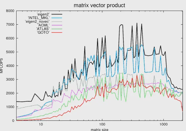
6.3 Eigen matrix vector product benchmark . . . 68

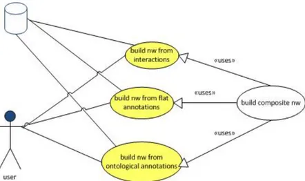
7.1 Use cases for the software architecture . . . 73

7.2 Direct network representation . . . 73

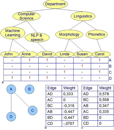
7.3 Examples of annotation profiles and their meaning . . . 75

7.4 Workflow of simple network construction . . . 79

7.5 Unfolding mechanism . . . 80

7.6 Workflow of the network composition process . . . 81

7.7 Main view of the system architecture . . . 83

7.8 Schema of the generic adapter pattern . . . 84

7.9 Xml file of a request to the software architecture . . . 85

7.10 Xml description of a sparsification method . . . 86

7.11 Sequence diagram associated to a network construction request . . . 87

(12)

7.13 Xml description of the sparsification method to be used . . . 90

7.14 Xml description of the annotation retriever to be used . . . 92

7.15 Xml description of the inputs of the network composition process . . . 93

7.16 Activity diagram associated to a user request . . . 94

7.17 Class diagram of Session and SessionRegistry . . . 95

7.18 Class diagram of the method registry . . . 97

7.19 Steps performed to find the maximum information content ancestor . . 105

8.1 Graphs of cache performances . . . 115

8.2 Percentage of time saved with annotation filtration . . . 120

8.3 Percentage of time saved with a smaller sparsification threshold . . . 121

9.1 Bar diagram of the annotated gene set frequencies . . . 124

9.2 ROC curves at different ranges of feature selection . . . 127

9.3 ROC curve for GO branches comparisons . . . 130

9.4 ROC curves for GO BP predictions from single networks . . . 133

9.5 ROC curves for GO BP predictions from composite networks . . . 134

A.1 Class diagram of the package cnw. . . 148

A.2 Class diagram of the package inputTypes. . . 149

A.3 Class diagram of the package Configuration. . . 151

A.4 Class diagram of the package DescriptionCreator . . . 153

A.5 Class diagram of the package methodDescriptor . . . 154

A.6 Class diagram of the retriever package. . . 155

(13)

List of Tables

8.1 Task performances for network from node associations . . . 112

8.2 Task performances for network from flat annotations . . . 113

8.3 Task performances for network from ontological annotations . . . 114

8.4 Table of the number of nodes and edges of the tested networks . . . . 116

8.5 Table of performances without annotation filtration . . . 118

8.6 Table of performances with annotation filtration . . . 119

8.7 Table of performances with less sparsified networks . . . 120

8.8 Table of performances with different filtration and sparsification setting 121 9.1 Data dimensions for the Gallus gallus species . . . 124

9.2 AUC results for different pruning configurations . . . 126

9.3 AUC results for different sparsity level . . . 127

9.4 AUC results for GO annotation predictions in Gallus gallus . . . 128

9.5 Table of annotations for the Arabidopsis thaliana organism . . . 131

9.6 AUC results for GO BP annotation predictions Arabidopsis thaliana -single networks . . . 132

9.7 AUC results for GO BP annotation predictions Arabidopsis thaliana -composite networks . . . 134

(14)

(15)

Chapter 3

INTRODUCTION

This section wants to provide a brief overview of the context in which this thesis is collocated. The main definitions, necessary for a correct understanding of this script, as well as descriptions of data types involved in the bioinformatics domain, and their related issues are provided.

3.1 Genes and Proteins

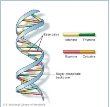
DNA (deoxyribonucleic acid) is a macromolecule which is present in each cell of almost all known living organisms. Its function is to code the instructions needed for cells development and functioning. The DNA structure is composed by two strands which run in opposite directions to each other; as discovered by James Watson and Francis Crick in the 1953, the two strands are arranged in two helical chains each coiled round the same axis (figure 3.1).

Figure 3.1 – DNA double helical structure. (Figure taken from http://ghr.nlm.nih.gov/handbook/basics/dna)

Each chain is composed by a sequence of simple units called nucleotides. Seg-ments of these nucleotide chains are responsible for carrying the genetic

(16)

informa-Chapter 3 Genes and Proteins

tion, they are named genes. Genes represent just a little part of the whole DNA in a cell, for example genes constitutes just the 1,5% of the human DNA whereas the remaining part has still an unknown function.

Figure 3.2 – Transcription and translation processes from DNA to proteins. During the

tran-scription phase, DNA is transcripted into mRNA which then leaves the cell nucleus towards cytoplasm. Here ribosomes drive the translation phase producing proteins. (Figure taken from [1])

Genetic information are encoded in the DNA through its structure, which is a long sequence of nucleotides, each one appearing in one of the four forms: (A)Adenine, (T)Thymine, (G)Guanine, (C)Cytosine. The ”instructions” coded in genes are used by cells for protein synthesis during the transcription and translation processes (fig-ure 3.2). At first each gene is transcribed into a macromolecule, called RNA (Ribo-nucleic acid), that is a (Ribo-nucleic acid as well; however its structure is composed by a single strand and the Thymine nucleobase is replaced by (U)Uracil. RNA is then used to transport the coding information outside the nucleus of the cell towards the cytoplasm. Here is where ribosomes translate RNA into a chain of amino acids. There exist different types of RNA, the one which is in charge of the genetic in-formation transportation outside the nucleus of the cell is called mRNA. While in prokaryotes mRNA is directly derived from DNA, in eukaryotes the transcript needs to be processed to produce a mature mRNA, this is because eukaryotes genes have both coding (exons) and non-coding parts (introns). In order to produce ma-ture mRNA the introns are removed and the exons are joined together, this process is called splicing (figure 3.3). The splicing process is often non deterministic and different mRNAs can be generated from the same pre-mature RNA (alternative spli-cing). The genetic information that are coded in the DNA are read (translated) by

(17)

Genes and Proteins Chapter 3

means of the genetic code which associates RNA triples to amino acids; each triple of nucleobase codes forms an amino acid, and sequences of amino acids form pro-teins. Since there are four different possible nucleobases in the DNA, the number of different generable triples is 64. However, the number of known amino acids is 20, hence the mapping between triples and amino acids is not univocal. The genetic code express such mappings between nucleotide triples and amino acids (figure 3.4 ).

Figure 3.3 – Transcription from nuclear RNA to messenger RNA (mRNA). In this phase introns

are discarded while exons are joint together. (Figure taken from [1])

(18)

Chapter 3 Genomic and Proteomic Research

The other fundamental entities componing the cell are proteins. They are the base elements of every biological structure, either plant or animal, and they parti-cipate in almost every process within the cell. They may have several functions ac-cording to their type: the most common ones are structural or mechanical functions, or else catalysing biochemical reactions. The main characteristic of proteins is their ability to bind other molecules, this allows proteins to carry out the set of functions they are known for. The binding feature is determined by the tertiary structure of pro-teins which, in turn, determines the presence of binding sites on the protein surface. A protein 3-dimensional structure can be described in four different aspects: the first one (the primary structure) is the amino acid sequence of the protein; the second aspect (secondary structure) is the presence of regularly repeated local structures; the third one (tertiary structure) expresses the overall shape of the protein by de-fining how secondary structures are combined together; the last aspect (quaternary structure) is the structure composed by several proteins to form a protein complex.

3.2 Genomic and Proteomic Research

Genomics is a discipline in genetics concerned with the study of the genome of or-ganisms. The term genome refers to the entirety of an organism’s hereditary inform-ation, including both genes and non-coding sequences of DNA/RNA. In particular, genomics focuses on the structures, contents, functions and evolution of the gen-ome. While genomics aims at studying the genome of organisms, proteomics, which is a scientific discipline that may be seen as the step further with respect of genom-ics, studies the proteome of organisms. More precisely, its aim is to characterise the structures, functions, activities and quantities of proteins in a species. Differently from the genome, the proteome is dynamic in time and its composition can vary due to external factors and/or kinds of cell or tissue. On the other hand, genome is nearly a constant entity; the interaction between genome and the environmental conditions, in addition to a particular phase of the cell life cycle and a specific organism cell or tissue, determines the proteomic expression in a given state. Due to the dynamic nature of proteome, proteomics is a discipline more complex than genomics.

The previously discussed process of protein biosynthesis is not error free, in fact the information coded by genes may be altered by external problems (i.e. adverse environmental conditions, such as electromagnetic radiation with high intensity, ex-cessive heat, etc.) and/or internal problems (e.g. unsolicited mutation, noise over the information transmission, etc.). These variations may cause problems to cells, diseases and, in the worst hypothesis, they can lead to the cell’s death. The proteo-mics and genoproteo-mics research areas are concerned with the molecular investigation of transcripts and proteins in order to gain a better understanding of biomolecular

(19)

Biomedical-Molecular Terminologies and Ontologies Chapter 3

mechanisms and interactions occurring inside a cell, and to provide the scientific community with new models describing the complex biology system of cells. How-ever, these field of studies are strongly multi disciplinary and involves disciplines such as biology, medicine, chemistry, electronics, statistics and informatics. In par-ticular, the last one targets the realization of tools and methods for the storage, management, analysis and visualization of a huge, every-day augmenting volume of data that are continuously generated by high-throughput experiments.

3.3 Biomedical-Molecular Terminologies and Ontologies

In the continuation of the thesis, the terms protein and gene will be often replaced by the term biomolecular entity due to the fact that the topics that will be exposed hold for both terms.

A controlled vocabulary provides a methodology to neatly organize knowledge in a way that it is easily readable and unambiguous, so that it can be correctly parsed by machines in a short time. A controlled vocabulary is composed by a set of terms, which are selected and authorized by the designer itself. This is diverse from the natural language, where the used vocabulary might allow for synonyms and poly-semes; these factors, which enhance the information ambiguity, are totally or nearly absent in a controlled vocabulary. Each term in a controlled vocabulary usually rep-resents a particular concept or characteristic, and it is univocally identified by an alphanumeric code. An example of controlled vocabulary is the Medical Subject Heading (MeSH) [3], its objective is indexing magazine articles and books to foster the categorisation and the research of scientific documentation within the medical domain. In the context of genomic annotations, there is a large number of controlled vocabularies which can be divided into two main categories:

• Flat controlled vocabularies: terms in these vocabularies are not linked to each other through relations;

• Structured controlled vocabularies or ontologies: terms in these vocabularies are hierarchically structured through relations, which are further characterized by a specific semantic meaning. The typical structure adopted for ontologies is the Direct Acyclic Graph (DAG)1.

While in the past the adoption of ontologies was rare, at present the number of tools which are working with ontologies have been increasing exponentially, hence their structures and properties are becoming of fundamental importance. However, there 1_{The word DAG stands for Directed Acyclic Graph. DAG is a mathematical structure represented}

by means of a graph having directed links and no cycles. Hence, for each vertex there exists no path that starts from a node and goes back to the node itself. DAG structures are often exploited to represent and describe ontologies.

(20)

Chapter 3 Biomedical-Molecular Terminologies and Ontologies

are still important controlled vocabularies which are flat; for example, this is the case of OMIM (Online Mendelian Inheritance in Man) [4], which is a vocabulary used to describe genetic pathologies in human organism, or the Reactome [5] vocabulary used for the description of pathways2. Among ontological controlled vocabularies, it is possible to cite ChEBI (Chemical Entities of Biological Interest) [6] focused on chemical components, the already cited MeSH [3], SBO (System Biology Ontology) [7] whose focus is on computational modelling within the biological field, or also GO (Gene Ontology) [8].

Nowadays, an always larger number of organizations are adopting controlled vocabularies to describe biomolecular entity knowledge. The mappings generated between biomolecular entities and specific terms, belonging to a controlled vocab-ulary, are called annotations. Hence, a certain entity is described by the meaning associated to the term that is annotating the entity itself.

Gene Ontology

The controlled vocabulary GO is part of the Gene Ontology project, which is per-haps the most important and used bioinformatics initiative, on a world wide scale. The final goal of the project is to standardize the way biomolecular entities are de-scribed, using methods that are independent of the particular species and/or type of biomolecular entities being described. As a matter of fact, the main outcome of the project is the GO ontology, however, besides that, the project supports also the implementation of tools that use the GO ontology for executing text mining tasks [9] or for clinical applications [10].

The GO ontology is a composition of three different ontological vocabularies, each one targeting a particular biological aspect of the cell; they are:

• Biological Process (BP): the biological process to which the biomolecular entity contributes (about 17000 terms);

• Molecular Function (MF): the biochemical function of the biomolecular entity (about 8600 terms);

• Cellular Component (CC): the location of the biomolecular entity in the cell (about 2500 terms).

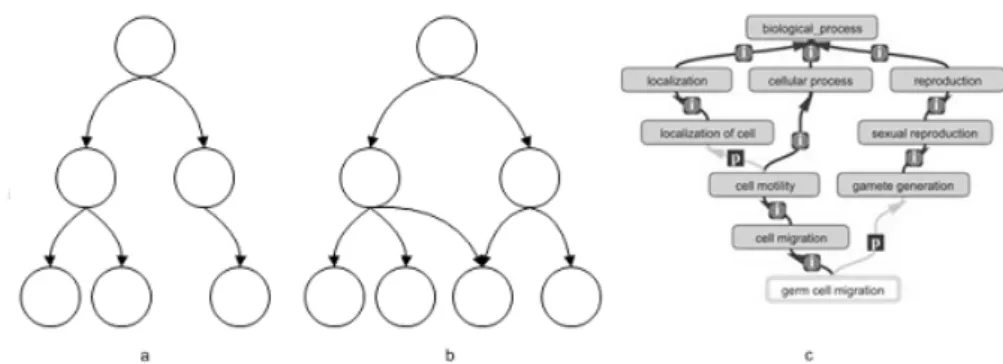
Each ontology can be represented by means of a DAG structure, the vocabulary terms are the nodes of the DAG, whereas the relations among terms (is_a and part_of relations) are encoded through links connecting two nodes (figure 3.5). All the three ontologies have just one root node each one, and the three root GO cate-gories (MF, BP and CC) have been designed to be independent ontologies.

(21)

Biomolecular Databanks Chapter 3

Figure 3.5 – DAG structure and Gene Ontology. a) A simple tree, b) A direct acyclic graph

(DAG). The third leave node has two parent nodes c) Fragment of the BP ontology. The term ”gem cell migration” has two parent nodes: it is part_of ”gamete generation” and it is a subtype of ”cell migration”

Besides defining the three ontologies, the GO Consortium freely provides also annotations to the biomolecular entities of forty seven different organisms. The as-sociation between a biomolecular entity and a specific vocabulary controlled term is usually performed by experts of the sector, called curators. Such a mapping (annota-tion) is derived through experimental results and/or literature reviewing. However, there are also cases in which annotations are not suggested by curators, instead they are computed electronically based on other annotations. In the GO ontologies this situation can be distinguished by looking at the Evidence Code associated to annotations; when a certain annotation has been computed electronically its Evid-ence code is IEA (Inferred from Electronic Annotation). The IEA annotations in GO are the only ones that are not reviewed by curators, as such they might be less accurate. Another important descriptor of an annotation to a GO term is the field Qualifier; in particular, the qualifier add information about the meaning of the asso-ciation, for example a qualifier with a value equal to NOT implies that the negate of the relation occurring between the term and the biomolecular entity has to be con-sidered. This is specially useful to indicate when an association between a term and a biomolecular entity should be avoided.

It is worthy to note that, depending on the meaning of the relations associated to the DAG structure representing an ontology, an annotation of a biomolecular entity to a specific controlled term can be ”unfolded” according to the DAG. The unfolding process consist in annotating the biomolecular entity also to the ancestors of the given term. On the GO ontologies, this operation is usually performed for links having a semantics of type is_a or part_of.

3.4 Biomolecular Databanks

Before personal computer’s coming, information was stored on physical support such as papers. Data storing was an expensive task due to the difficulties

(22)

en-Chapter 3 Biomolecular Databanks

countered in managing and ordering large quantities of data, thus the economic, time and human resources needed for these tasks were considerable. With birth of informatics and its quick evolution, new ways of data management have been proposed and developed. In particular, databases turned out to be an effective and efficient solution to manage data. A database, or databank, is a set of information where data are typically stored and organized in a neat and structured way. The core part of a database, which is responsible for these operations, is its DBMS (database management system). By putting structural and logical constraints upon the inform-ation representinform-ation, the DBMS allows other applicinform-ations to efficiently and effectively manage and query data. The recent techniques used in biomolecular experiments have been generating an unprecedented quantity of new genetic data (e.g microar-ray experiment [11, 12]), therefore one of the most important bioinformatics goals is to find efficient solutions to manage experimental data. Databases are the natural way to face this problem, hence it is not surprising that they cover a central role in bioinformatics. However, the problem is far to be completely resolved, mainly due to further issues that are intrinsic to the scientific research nature of the problem. In fact, many research groups are involved in genomic and proteomic projects, and often each of them is independently carrying out its experiments, obtaining its own results; the scientific community needs to have access to a global view of the know-ledge disclosed from single experiments, thus the efforts of bioinformatics are not just seeking methods to manage large dimension of data, but they are also con-cerned with the devising of new techniques to integrate data from different sites. The final objective is to create simple interfaces, usable by researches, which per-mit to share all the information among the scientific community. In this scenario, the integration of data from several databases is of fundamental importance, but unfor-tunately this task is not simple and it is hampered by the lack of standards within the biomedical community. Data are often stored using different technologies, formats and terminologies, hence there is not a simple and common solution to this prob-lem, instead many approaches to tackle these issues have been proposed, each one with its own feedbacks and drawbacks. The project GPDW [13], carried out by our laboratory, is collocated in this respect and it faces the problem by suggesting a data warehouse approach.

There exist several technologies available for databases [14, 15], the most com-mon used technologies in bioinformatics domain are:

• flat file: all data are stored in a unique file. All the records are stored sequen-tially, separated by special characters; usually records are arranged in tabular like structures, where each record is a row and each column is a property that describes the record;

(23)

• relational database: data are conceptually arranged in tables which are linked together through relationships. The DBMS is in charge of resolving those re-lationships and for the addition, modification and deletion of tuples (records). [14, 15]

Biological databanks contain data coming from a wide spectrum of molecular biology sectors and they can be divided in two groups:

• primary databanks: they store information and annotations about DNA se-quences, proteins and their structures. The stored biomolecular sese-quences, and their respective annotations, should be enough to identify a particular sequence along with its function. A few examples of primary databanks are GenBank [16], EMBL [17] and DDBJ [18];

• secondary databanks: they contain enriched information derived from primary databanks. Examples of information stored in secondary databanks are RNA, pathways, data from microarray experiments [11, 12], pathologies etc. Per-hapts, the most known secondary databanks are OMIM [4] and PUBMED [19].

Since there exist many dimensions through which is possible to describe biomolecu-lar entities, specialized content databases have been proposed, such as:

• databanks for scientific literature;

• databanks for taxonomies;

• databanks for nucleotides;

• databanks for genomes;

• databanks for proteins;

• databanks for microarray data.

As showed in figure (3.6), the number of biological databanks has been subject of a tremendous increment over the time.

(24)

Chapter 3 Biomolecular Databanks

Figure 3.6 – Growth of biological databank number over the time. (Figure taken from [1])

Another distinction among existing databases can be arranged according to the way they are accessed. The plurality of possible database access methods is an-other layer of complication that must be taken into account when integrating different databanks. Typical way for accessing databanks are:

• Access through web interfaces (HTML or XML pages): information provided is not structured and data are showed by means of heterogeneous interfaces. Customized parser are necessary to retrieve data;

• Access through FTP servers: this method requires to have human and tech-nological resources to re-implementing a local databank;

• Access through web services: this service is made available by just a few databanks; executable queries are limited to the ones offered by services;

• Direct accesses: it is almost never available due to the potential damage to which databanks would be exposed.

Data File Formats

Databanks may provide the same data in different formats and a unique standard to represent and share information related to biomolecular entities, and their an-notations, is missing [20]; figure (3.7) shows the most common cases of data file formats. A flat format is a text file containing data values in which the structure of data is defined by rows and special characters. Usually, within the genomic context, every row of a flat file is associated with a specific biomolecular entity, and the row

(25)

meaning is defined by one or more labels, sometimes having hierarchical relation-ships with each others. Generally speaking, when data values are organized in rows and columns, a flat file can be seen as a textual file in a tabular-like form where the semantics of data depends on the their position in the table. The existent variations of tabular file are schematically illustrated in figure (3.8).

Figure 3.7 – Genomic data file formats. (Figure taken from [20])

Figure 3.8 – Tabular data file formats. (Figure taken from [20])

Other databanks provide their data by means of SQL dumps. Since dumps are DBMS specific, even importing data with the precedent versions of the right DBMS might be problematic. Examples of databanks which make available SQL dumps of their data are GO (Gene Ontology) [8] and InterPro [21], this latter one is a database that stores information about protein family domains and functional sites.

XML (eXtensible Markup Language), is a metalanguage created and managed by the World Wide Web Consortium (W3C). Its purpose is to define languages for describing semi structured documents but, due to its flexibility, it has been used also for communication of data between heterogeneous sources and destinations. For these reasons many databanks provide their data in a XML format. The structure of a XML document can be described using the language ”Document Type Definition” (DTD) or by means of XML-Schema which, compared to DTD, has the advantage of being a XML derived language itself [14].

(26)

Chapter 3 Issues Related to an Effective Use of Available Biomolecular Information

Another format, that sometimes is made available by biological databanks, is RDF (Resource Description Framework). RDF is the standard proposed by W3C to describe structured metadata in order to enhance interoperability among applic-ations which communicate through the Web. Using RDF it is possible to specify a RDF model which describes the meaning of the data by defining meta data and re-lationships among them; a particular RDF model is the RDF Schema, which defines syntax and constructors to specify the structure of the metadata, thus defining the semantics of a RDF model. [22]

3.5 Issues Related to an Effective Use of Available Biomolecular Information

From what it has been said so far, it is possible to summarize the issues that come up when dealing with biomolecular information: First of all, there are a lot of databanks geographically distributed, this fact introduces problems related to the integration of data from heterogeneous databases and the resolution of duplicated and incon-sistent data. The work of the last years has been focused on the integration of biomolecular information in a unique central structure, thus easing the updating and management tasks of data, this was also one of the goal of GPDW [13] and other integration systems; another issue is represented by controlled vocabularies. In fact, even tough they claim to be orthogonal to each others, there are relations among terms of one vocabulary with terms of other vocabularies, specially if they are managed by different organizations; finally, there is a problem with the goodness of annotations included in databanks [23] and the difficulties faced by curators in valid-ating, maintaining and managing new annotations. For example, the Go Consortium has annotated just 19920 genes out of the about 25000 present in human beings from the completion of human genome sequencing [24] finished in 2003 by Celera-Genomics and Homo Genome Project (HGP) to nowadays. Furthermore about the 58% of the current annotations are electronically inferred, this means that they have not been confirmed by any curators, so they might have a low accuracy.

3.6 Complex Networks Analysis

The other hot topic related to biomolecular data is the correct interpretation of the data themselves. In fact, the recent explosion of the amount of experimental data, derived from large-scale experiments, has brought new challenges when trying to analyse them. High-throughput techniques in molecular biology generate a huge amount of data which can potentially reflect the interplay between biomolecules on a global scale, however the complexity of the mechanisms governing the cell life and the volume of the available data make hard to characterize roles and relations of biomolecules. What is needed are models, frameworks and techniques which

(27)

Complex Networks Analysis Chapter 3

can accommodate and exploit the richness of information available from the scien-tific community to discover new knowledge about cells and their members. To this end, network models provide a natural, flexible and expressive formalism to model and analyse the cell environment and its complex interconnections. The represen-tation of complex cellular networks by means of graphs has made it possible to study topological and functional features of the cells using well understood graph theoretical concepts that can be used to predict the structural and dynamical prop-erties of the underlying network. Using graph driven methods for analyzing complex cellular network it is a rather recent field of studies, nevertheless several methods and approaches can be found in the literature. Some works have been done (e.g. [25, 26]) trying to review and organizing the constantly growing amount of proposed approaches, methods and tools, whose common aim is to extract information from biological data using a graph-based framework.

Basically, two major categories of biomolecular networks can be distinguished: networks which reflect the biomolecular physical interconnections that play some role within the cell environment, and the one whose links are logical associations among biomolecular entities (i.e. genes and/or proteins). In both cases the nodes of the networks are typically associated to cellular components, whereas the edges change accordingly to the meaning they express.

The most common biological networks belonging to the first group are:

• Transcriptional gene regulatory networks: they are represented by graphs with two sets of vertices. One set represents transcription factors and the other represents genes. Each edge symbolizes a binding of a transcription factor to a gene;

• Protein-Protein Interaction networks (PPI): they consist of the physical interac-tions (edges) among an organism’s proteins (nodes);

• Metabolic networks: each vertex represents a metabolite and each edge rep-resents a biochemical reaction.

On the other side, the second category of networks is composed by networks whose edges semantics is not constrained to represent physical phenomena occurring within the cell. For example, two genes might be linked together if they are known to have the same function within the cell. Typical instances of this class of networks are:

• Co-Expression networks: they describe expression patterns among genes. Nodes are genes, and two genes linked together with an edge means they are expressed under the same conditions;

(28)

Chapter 3 Complex Networks Analysis

• Functional networks: they represent functional associations among nodes (i.e. proteins or genes) by means of edges;

• Disease-Gene networks: they are represented by bipartite graphs with two sets of vertices. One set represents diseases of a given organism, while the other represents the organism’s genes. A gene and a disease are connected by an edge if the gene is involved in the disease.

Throughout this thesis particular attention was paid to the class of functional net-works, as a matter of fact the tests performed in this project all concern functional networks computed from data derived from the GPDW data warehouse of Politec-nico di Milano[13].

Biological Network Reconstruction

There are two main approaches for network reconstruction differing in the underlying data types and interpretation. On the one hand, networks are reconstructed based on genome information, well-curated databases and primary research literature; on the other hand, networks are inferred, usually from gene expression experimen-tal data. With the former approach, semantically controlled extraction of database instances leads to networks based on carefully organized knowledge gathered in many in vitro and in vivo experiments. However, data collected from databases usu-ally lack of tissue and/or disease specific information (they are concerned with a the-oretical whole genome stem cell) and information about temporal processes, thus if the analysis focus is constrained to certain tissue specific or temporal aspects, net-works reconstructed from databases may present undesired links (e.g. molecules can be connected although they are no simultaneously highly expressed in any tis-sue). The second approach involves the prediction of interactions starting from a set of experimental data, usually gene expression profiles. This method is more suitable for those analysis which want to study cell aspects under certain conditions and/or dynamical perturbations of the environment. Also in this case, networks might show incorrect interactions due to the nature of the reconstruction mechanism itself, which is based on prediction of interactions.

Several resources, depending on the network interaction types that have to be modelled, can be exploited for network construction. Maps of interactions are al-ready present in the literature (e.g.[27, 28, 29, 30] are maps of protein interaction networks; also a metabolic network reconstruction for S. cerevisiae is available at [31]), these maps are usually concerned about a single organism and a single in-teraction type (i.e. Protein-protein inin-teractions, gene-gene regulatory inin-teractions or metabolic interactions). The interactions among genes/proteins are collected by integrating the results of several experiments and those data are usually stored in

(29)

Complex Networks Analysis Chapter 3

specialized databases which provide the information necessary to build networks (e.g. DIP [32], BioGRID [33] or STRING [34] for protein-protein interactions, KEGG [35] and BioCyc [36] for metabolic networks, and RegulonDB [37] and EcoCyc [38] for transcriptional regulatory networks).

Besides directly collecting network interactions from data, one might use the data available in the literature and/or in data sources to infer networks. Network inference is the inference of the topology, that is the prediction of the "wiring diagram" of the network. Usually the inference of a biological network structure is done by using the growing sets of high-throughput expression data profiles. However, other promising approaches can be found in the literature, they usually try to infer an a-priori determined type of related links; for instance, focusing on functional networks, the assumption behind the presence of a connection between two network entities is that they share some common cellular functions. These type of edges are often derived by learning from a so called golden standard [39, 40]; in this respective, the Gene Ontology’s[8] Biological process branch is probably the most common used source of functional information.

This thesis tries to answer in an efficient and effective way to some of the prob-lems arising in the biomedical context by adopting a network approach to model the data taken from the GPDW data warehouse developed at Politecnico di Milano.

(30)

(31)

Chapter 4

THEORY OF COMPLEX NETWORKS

Biological systems, neural networks, scientific co-authorship, transportation net-works are just a few examples of systems that can be expressed by means of graphs. These systems are characterized by the presence of discrete units and interconnections among them. Representing a system with a graph allows to spec-ify and investigate its global and local properties; in order to describe a system with a graph, one needs to specify its nodes (discrete units) and edges (interconnections) among them. The following sections want to provide basic notions about graph the-ory and complex system properties, as well as metrics which will be necessary to understand the work discussed throughout this script.

4.1 Graph Definition

The study of networks has been part of a branch of discrete mathematics for decades, this discipline, in the mathematics domain, is called Graph Theory. However this field of studies was confined to the study of small networks which have a formal math-ematics description. With an always larger computational power made available by recent progress in discipline such as computer science, electronics and informat-ics, a new movement of interest and research is appealing the scientific community: Complex Networks. Unlike graph theory, the discipline of complex networks analyse networks whose structure is irregular, complex and evolving in time. Moreover, the networks under investigation often encompass thousands or millions of nodes, thus moving the attention from properties of individual edges or nodes to the large scale statistical properties of graphs. Here, the formal definition of a graph, taken from the graph theory area, is given.[41] Since a complex network can formally be repre-sented as a graph, providing the reader with a mathematical description of what a graph is might be useful to better understand the next chapters.

Basically a graph G = (N ,L ) is composed by two sets N and L , where N 6= Ø andL is a set of pairs of elements of N . A graph can be directed or undirected, in the former case elements of L are ordered pairs while in the latter one there is no specific direction in relationships between the two elements of the pair. The elements ofN ={n1, n2, ..., nN} are nodes (or vertices) of the graph G, while links (or

(32)

Chapter 4 Graph Definition

andL are indicated with N and K, respectively. In the following sections a graph will be denoted as G(N, K) = (N ,L ) or simply GN,K. Usually a specific node is denoted

with its order i in the set N , hence a natural way to refer to a determined link is to specify the nodes it connects together. li, j is the link which couples nodes i and j,

the link is said to be incident in nodes i and j; whereas the two nodes are referred to as the end-nodes of link li, j. Two nodes joined by a link are referred as adjacent

or neighboring. Figure (4.1)

Figure 4.1 – Graphical representation of an (a) undirected, (b) directed, (c) weighted undirected

graph. (figure taken from [41]).

shows the usual representations of graphs. As it is possible to observe from the figure (4.1), links in directed graphs are represented with arrows which draw the direction of the relationship between two nodes. Labels Wi, j of graph (c)

repre-sent weights of links joining node i and j; weights are graphically denoted with the thickness of edges. Weighted networks provide a model to describe the strength of connection; in many real network examples this is a desirable feature, for instance it is possible to represent unequal traffic on the Internet [42], strong and weak ties be-tween individuals in social networks [43, 44] or different capabilities of transmitting electric signals in neural networks [45] and many other scenarios. The graph defini-tion exposed above can be further enriched to encompass domain specific detailed. For instance there may be the necessity to separate nodes and/or edges accord-ing to their characteristics, in other words, sometimes we would like to represent different types of nodes and edges. This could be the case of a social network of people, the vertices may represent men or women, people of different nationalities, locations, ages and so on. Edges may represent friendship, animosity, professional acquaintance and many others. A special case of graphs formed by two different types of nodes are bipartite networks (figure 4.2)

(33)

Graph Definition Chapter 4

Figure 4.2 – (a) is an example of bipartite network, nodes denoted with letter belong to the

same class, whereas nodes referred with numbers belongs to another one. (b) represents the projection of the bipartite network onto the class of nodes indicated by letters (a). (figure taken from [46]).

. A bipartite graph B = (V ,E ) is composed by two sets of nodes V1,V2such that

V1∩V2= Ø and one set of links E where if the link ei, j ∈E then i ∈ V1and j ∈V2,

or the reverse. Hence in a bipartite networks links can join just nodes belonging to different classes. Examples of systems where this formalism could be useful are the real world associations papers/authors, boards/directors or actors/movies. From a bipartite network is possible to obtain an ordinary graph by projection (figure 4.2), in the projected network the link li, j will exists iff the the two nodes i and j have

a common neighbor in the bipartite network, so if exist a node z such that ei,z and

e_j,z are links of the bipartite graph. Finally, another aspect that complicates the formalism used to describe graph, but at the same time allows for more powerful descriptions of systems, is the time. In fact many system are not static and their component may evolve over time, hence vertices or edges may appear or disappear, as well as values defined on those vertices and edges may change.

Graph Notations

The maximum number of edges for a graph G with N nodes is N(N − 1)/2 (N(N-1) for directed graph ), when this is the case the number of edges K = ϑ (N2)and the graph is said to be dense, whereas when K ϑ (N2) the graph is called sparse. It is often desirable to analyse only portions of a graph, which are properly called subgraphs; a subgraph G0= (N 0,L0) of a graph G = (N ,L ) is a graph such that N 0_⊆_{N and L}0_⊆_{L . If G}0 _{contains all links of G that join two nodes in}_N 0_{, then}

(34)

Chapter 4 Networks Properties

G0 is said to be the subgraph induced byN 0. Other terms that are recurrently used in graph theory refer to the concept of reachability among nodes; two nodes that are not adjacent may be nevertheless reachable from one to the other. A walk from node i to j is defined as a sequence of adjacent nodes that starts with i and ends with j. A walk is often associated with a number which specified the walk length and it is computed as the number of edges in the sequence. Other three notations are derived from the concept of walk: the first one is trail, which is a walk without edge repetition; the second one is path that is a walk in which no node is visited more than once; the last one is cycle which is a closed walk, of at least three nodes, in which no edge is repeated. One property that is often analysed in a graph is the shortest path or, also called, geodesic, that is the walk of minimal length between two nodes. Finally, a graph is defined as connected if for every pair of distinct nodes there exists at least one path between the two nodes; if a graph is not connected then it is said do be unconnected or disconnected. A component of the graph is a maximally connected induced subgraph, where maximally means that it is impossible to find a connected induced subgraph which includes all the nodes of the component; a giant component is a component whose size is of the same order of N.

Adjacency Matrix

A common representation of a graph is the adjacency matrix. Given a graph GN,Kits

adjacency matrix is a square matrixANxN whose entry ai, j is equal to 1 when the link

l_{i, j} exists, and zero otherwise. A weights matrix may also be defined for weighted networks, in this case the entry wi, j will take the value of the weight corresponding to

the link li, j. Further possible representation will be discussed later on in the chapter

“Materials and Methods”

4.2 Networks Properties

Since the beginning of interests and researches in complex networks, many net-works have been analysed and compared. Perhaps the first observation that came out from these comparative efforts is that real world networks are non random in some features. A first issue that research had to face was how to compare net-works. For this reason a serie of new concepts and measures were proposed to characterize real network topologies. Global measures such as degree distribu-tion, diameter, characteristic path length, clustering coefficient and modularity have been also widely discussed in the context of cellular networks [47, 48]. This section presents the unifying principles and the statistical properties common to most real networks, maintaining a special attention towards biomolecular data applications; the reader interested in a more detailed discussion of these properties could consult

(35)

Networks Properties Chapter 4

[41, 49, 46].

Node Degree

The degree ki of a node i is the number of links incident with the node:

k_i=

_∑

ai, j j∈N

(4.1)

where ai, j is the term of the adjacency matrix in position (i, j). The degree node

must be divided in two distinct measures in case of directed networks, these two measures are called out-degree kout

i of the node and in-degree kini of the node and

they count just the outgoing and ingoing edges of the node, respectively. The total degree k is obtained by summing up in-degree and out-degree. In a weighted graph is possible to re-define the concept of node degree taking into account weights of the links incident to the node. In this case the metric adopted is called strength si of

the node and it is computed by summing up the weights of incident edges:

si=

∑

wi, j j∈N

(4.2)

Degree Distribution

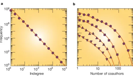
The degree distribution P(k) is the probability that a node chosen uniformly at ran-dom has degree k. It is the most basic topological characterization of a graph. As it was for the degree node in directed networks, the degree distribution is also split in two distributions P(kin)and P(kout). Degree distributions are often plotted (figure 4.3)

(36)

Figure 4.3 – Degree distributions for real networks. a)World-Wide Web. Nodes are web pages;

links are directed URL hyperlinks from one page to another. The log–log plot shows the number of web pages that have a given in-degree (number of incoming links). b) Co-authorship net-works. Nodes represent scientists; an undirected link between two people means that they have written a paper together. The data are for the years 1995–1999 inclusive and come from three databases: arxiv.org (preprints mainly in theoretical physics), SPIRES (preprints in high-energy physics) and NCSTRL (preprints in computer science). Symbols denote different scientific com-munities: astrophysics (circles), condensed-matter physics (squares), high-energy physics (up-right triangles) and computer science (inverted triangles). (Image taken from [50])

to gain an idea on how the degrees are distributed among the nodes. Without plotting the distribution it is still possible to summarize its characteristics by using the n-moment of P(k):

< kn>=

_∑

k

knP(k) (4.3)

The 1-moment of P(k) is the mean degree of G.

In a weighted network, given a node i, two different situations can occur concern-ing its weights: all weights wi, j can be of the same order _ksi_i, or only a few weights

dominates over the others. This disparity on weights of a node i can be evaluated by the measure Yi[51]: Yi=

∑

j∈Ni (wi, j s_i ) 2 _(4.4)

whereNi is the set of first neighbor of node i. Similarly to the degree distribution

for degree nodes the strength distribution R(s) defines the probability that a vertex has strength s.

Shortest Path Lengths

Shortest path is another basic measure used to characterize network topologies. This feature plays an important role in those networks where communication and

(37)

transport problems are important. To summarize the length paths of a network an average shortest path length L, also known as characteristic path length, is often calculated:

L= 1

N(N − 1)_{i, j∈N ,i6= j}

∑

di, j (4.5) where di, j denotes the geodesic distance between node i and node j. The

prob-lem of 4.5 is that it diverges if two nodes are not connected in any way (di, j → ∞).

To avoid this circumstances one can limit the summation in formula 4.5 to the nodes belonging to the largest component, another alternative is to consider the harmonic mean of geodesic lengths, calculating the efficiency of G:

E= 1

N(N − 1)_{i, j∈}

∑

_{N ,i6= j} 1 di, j

(4.6)

When using the efficiency, instead of the characteristic path length, the nodes that are not connected contribute with zero value in the summation. The efficiency is an indicator of the traffic capacity of the network. In case of weighted networks, lengths can be associated to each edge (the edge length in unweighted networks is assumed as equal to 1), for instance one could define the length of edge which goes from i to j as li, j=_{wi, j}1 . Having length associated to edges the definition of geodesic

distances changes for taking into account this fact, the quantity di, j, called weighted

shortest path, is now defined as the the smallest sum of edge lengths throughout all the possible paths in the graph from i to j. A diameter of a network is defined as the maximum value over every possible geodesic distance/weighted shortest path of the network.

By observing at the diameters and average path lenghts of biomolecular net-works [52, 53, 54], it has been observed that these two values are often ’small’ in comparison to the network size. This property is known as small-world property and is not peculiar of only biomolecular networks its usual interpretation in this context is that only a small number of intermediate reactions are necessary for any one protein/gene/metabolite to interact with another one.

Clustering

Clustering is a measure used to compare the transitivity T of a network, where the transitivity refers to the relative number of transitive triples:

T = 3 × #o f TrianglesInG

#o f ConnectedTriplesO f VericesInG (4.7) This is the ratio of triangles in the network over the whole number of triads. The factor 3 in formula 4.7 accounts for the fact that a triangle can be seen as three

(38)

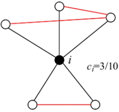
different triads. Another metric proposed to evaluate the transitivity property of a network is the clustering coefficient C. Differently from 4.7 C is calculated starting from a local property of the graph: the local clustering coefficient of a node ci (figure

4.4)

Figure 4.4 – Example of local clustering coefficient of node i in an undirected, unweighted

network. (figure taken from [46])

. This quantity is defined as:

c_i= 2ei k_i(ki− 1) = ∑ j,m a_{i, j}a_j,ma_m,i k_i(ki− 1) (4.8)

The local clustering coefficient states how likely two nodes j,m that share a com-mon neighbor i are connected to each other. In 4.8 eirefers to the number of edges

which are present in the subgraph induced by the neighbors of i. The clustering coefficient of the whole graph is then given by the mean of all local clustering coeffi-cients:

C= 1

N_i∈

∑

_Nci (4.9) It is possible to investigate the variation of local clustering coefficients according to the node degrees by defining the quantity c(k) as the average of local clustering coefficients of nodes having degree equal to k. Besides the clustering coefficients discussed above many other metrics have been proposed over the years, Barrat et al. [55] proposed a cluster coefficient that takes into account weights of a weighted network:

cW_i = 1 si(ki− 1)

∑

_j,m

(wi, j+ wi,m)

2 ai, jaj,mam,i (4.10) The weighted clustering coefficient accounts for the number of closed triangles in the neighborhood of node i as well as their relative weight with respect to the vertex strength.

(39)

One example of a clustering analysis study is the work of Ravasz et al. [56]; in this work the average clustering coefficients C for the metabolic networks of 43 organisms were compared with the average clustering coefficient of a random net-work with the same degree distribution. In all the 43 cases the average clustering coefficient of the metabolic network was at least one order of magnitude higher than the one of the random network implying that in metabolic networks edges tend to be clustered together.

Communities

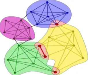
Many complex networks can be characterized by their attitude to be divided into communities. The intuitive behind the idea of community concept is that nodes tend to be more connected within the community they belong to. There is not a clear definition of community in the literature but the two features that are used the most to identify communities are: 1) groups of vertices that have a high density of interconnections within them, with a lower density of edges among different groups (figure 4.5)

Figure 4.5 – Three communities with high density of intra-community connections and low

den-sity of inter-community connections. (figure taken from [41])

; or 2) groups of nodes which are fully, or nearly fully, connected within the same groups. The second feature brings to the definition of cliques, k-plex and n-clique. A clique is a maximal subgraph of G in which each node of the clique is connected to every other node belonging to the same clique. The definition of clique can be weakened requiring that the maximum number of missing links for each node, with respect to a maximal complete subgraph (clique), is k, in this case the maximal subgraph obtained takes the name of k-plex. A different definition for characterizing communities, which is derived from the clique definition as well, is the n-clique. A n-clique adopts the same definition of a clique with the exception that the adjacency of nodes is substituted with a reachability requirement of at most n. More details on

(40)

community structures, definitions and algorithms to deal with them are provided in the next sections.

Graph Spectra

The set of eigenvalues of a graph adjacency matrix A , the so called graph spectra, is another mechanism to characterize graph. A graph GN,K has N eigenvalues and N

corresponding eigenvectors. The graph spectra present some features depending on the topology of the graph; undirected graphs, without loops, have real eigen-values and the corresponding eigenvectors are orthogonal to each other, whereas imaginary eigenvalues can arise from directed graphs. From the Perron-Frobenius derives the fact that directed and undirected graphs have a real eigenvalue µN which

is associated to a real non negative eigenvector, in addition the absolute value of all the other eigenvalues is less or equal than µN. If G is connected then µN has

multi-plicity 1 and |µ| < µN where µis a generic eigenvalue ofA different from µN . The

value of µN decreases with edges and nodes removing, in a connected undirected

graph this means that µN is not degenerate and every component of the

corre-sponding eigenvector is non-negative, since the other eigenvectors are orthogonal to it their components are mixed in signs. Eigenvalues and eigenvectors of an ad-jacency matrix have properties strictly related to network topology characteristics, such as diameter, connectivity of graph and cycles.

4.2.1 Topology of Real Networks

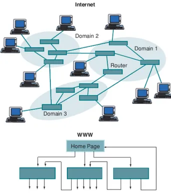
Nowadays, the availability of large databases and high computing power has per-mitted to construct large real network and to analyze their properties. Many real systems can be modeled by using complex networks, this in turn, allows to investi-gate topological and dynamical features of systems. Examples of systems that have been modeled by using complex networks, thus identifying edges and nodes for the systems, are numerous. The World Wide Web (WWW) is a network of websites (fig-ure 4.6), the brain is a network of neurons, an organization is a network of people and also food webs and metabolic pathways can all be represented by networks (fig-ure 4.7)[57]; a first stage in complex networks researches was to analyse, compare and characterize large real network topologies. This process led to interesting dis-coveries, finding that most of real network topologies share common features which are not present in regular graphs (those that had been studied by mathematician in graph theory), and they are not even in completely randomized graphs.[41] The two main topological characteristics that have been found in real networks are the so called small-world and scale-free properties.

(41)

Figure 4.6 – Network structures of the Internet and the WWW. On the Internet, nodes are routers

(or domains) connected by physical links. The nodes of the WWW are web pages connected by directed hyperlinks. (figure taken from [57])

(42)

Figure 4.7 – (a) Food web of the Little Rock Lake shows “who eats whom” in the lake. The

nodes are functionally distinct “trophic species”. (b) The metabolic network of the yeast cell is built up of nodes - the substrates that are connected to one another through links, which are actual metabolic reactions. (c) A social network that visualizes the relationship among different groups of people in Canberra, Australia. (d) The software architecture of the Java Development kit 1.2. The nodes represents different classes and a link is set if there is some relationship (use, inheritance, or composition) between two corresponding classes. (figure taken from [57])

Small-World Property

The small-world property of a network refers to the fact that there is a relatively short path between any two nodes of the network. Its characterization is given by an average shortest path length L (see Eq. 4.5) that depends at most logarithmically on the network size N.[41] Many real networks have been shown to have the small-world property, as well as an high value of the clustering coefficient (see Eq. 4.9). This fact is at the basis of the proposal made by Watts and Strogatz [58], they define a small-world network as a network having a small value for the average shortest path and high value for the clustering coefficient. In addition to define the small-world property, the authors also proposed a network model which generates network with such characteristics.

Scale-Free Property

Another features that a lot of large-scale complex networks have in common is the scale-free property. This property refers to the fact that a network display power law shaped degree distribution P(k) ∼ Ak−γ. The name scale-free is due to the fact