ALMA MATER STUDIORUM - UNIVERSITÀ DI BOLOGNA
FACOLTA’ DI INGEGNERIA
CORSO DI LAUREA SPECIALISTICA IN INGEGNERIA CIVILE
D.I.S.T.A.R.T.
DIPARTIMENTO DÌ INGEGNERIA DELLE STRUTTURE, DEI TRASPORTI, DELLE ACQUE, DEL RILEVAMENTO, DEL TERRITORIO
TESI DI LAUREA in
Tecnica delle Costruzioni LS
DYNAMIC TESTS AND STRUCTURAL
IDENTIFICATION OF THE DOWLING
HALL FOOTBRIDGE
CANDIDATO: RELATORE:
Chiar.mo Prof.
Stefano Sensoli Claudio Ceccoli
CORRELATORI: Prof. Ing. Tomaso Trombetti Prof. Ing. Babak Moaveni
Anno Accademico 2008/2009 Sessione III
Ai miei genitori, per aver reso possibile la bellezza di questi anni. Ai miei amici, per avermi accompagnato ed abbracciato.
Index
Introduzione ……… Introduction ……… 1. Test ………. 1.1. Test structure ……… 1.2. Instrumentation ………1.3. Dynamic tests performed ……….
1.3.1. April test………..
1.3.2. June test………...
2. Raw Processing of the experimental data ………...
2.1. Filtering ………
2.2. Down-sampling ………
2.3. Fourier transform and Power Spectral Density …….……... 3. Modal Analysis ………...
3.1. Peak-Picking ……...………
3.1.1. Method ……….
3.1.2. Identification results ………
3.2. Natural Excitation Technique combined with Eigensystem Realization Algorithm (NEXT-ERA) ………..
3.2.1. Natural Exitation Technique (NExT) ………..
3.2.2. Eigensystem Realization Algorithm (ERA) …………
3.2.2.1. Discrete-Time State-Space System
Representation……… 3.2.2.2. Markov Parameters and Weighting Sequence..
3.2.2.3. Controllability and Observability ………
3.2.2.4. Hankel Matrices ………...
3.2.2.5. Eigensystem Realization Algorithm (ERA) …
3.2.2.6. Transformation of ERA Realization to
Continuous Time ………... 7 13 17 17 19 21 21 25 29 30 33 35 41 41 42 45 48 48 56 56 58 59 60 62 63
3.2.2.7. Advantages of the ERA realization…………..
3.2.3. Identification results ………
3.3. Comparison of the April and June tests experimentally identified modal parameters ………. 4. Test Analysis Correlation ……….
4.1. Finite element model ………
4.2. Calibration of the finite element model based upon the analytical experimental correlation study ………
4.3. Comparison of FE predicted and experimentally
identified modal parameters ………... Future work: the continuous monitoring system project ... Conclusions ……….. References ……… Appendix A ……….. Appendix B ……….. 66 68 71 75 75 77 79 83 85 87 91 107
7
INTRODUZIONE
Questo lavoro riguarda la progettazione e la realizzazione di due test dinamici eseguiti sul Dowling Hall Footbridge, sito presso il campus centrale della Tufts University, Medford, USA. Dai dati rilevati nei due test, è stato possibile, attraverso l’implementazione di adeguati algoritmi di calcolo, identificare le caratteristiche dinamiche della struttura e aggiornare e affinare il modello numerico agli elementi finiti creato per simulare il comportamento strutturale.
I test dinamici sono strumenti ampiamente utilizzati nell’ingegneria civile per identificare le caratteristiche dinamiche delle strutture (frequenze naturali, coefficienti di smorzamento, forme modali). Negli ultimi decenni si è riscontrato un interesse crescente intorno a quest’ambito, sia per la notevole attenzione suscitata dalla progettazione di strutture in zona sismica, sia per la possibilità di verificare e affinare modelli numerici grazie ai risultati ottenuti dalle prove sperimentali.
I test dinamici sono operativamente realizzati attraverso l’applicazione, in posizioni specifiche e accuratamente pianificate, di sensori capaci di rilevare molteplici tipologie di parametri, ambientali ( temperatura, umidità, ecc.) e strutturali (accelerazioni, velocità, ecc.), che consentano una descrizione approfondita e completa di tutti i fattori che caratterizzano il comportamento della struttura sottoposta alle diverse tipologie di sollecitazione. In particolare è possibile identificare due diverse modi di svolgimento dei test, in cui la struttura risulta eccitata attraverso azioni di tipo ambientale (vento, traffico, pedoni) oppure attraverso l’utilizzo di appositi dispositivi meccanici che generano input dinamici programmati (shakers, vibrodine, ecc.). In entrambi i casi è possibile identificare le caratteristiche dinamiche facendo uso di appropriati algoritmi per l’identificazione strutturale che interpretino
8
correttamente gli output della struttura a seguito della sollecitazione impressa.
Per il caso in esame, i test sono stati condotti utilizzando un’eccitazione di tipo ambientale e registrando la risposta della struttura attraverso dodici accelerometri disposti sull’intera lunghezza della passerella pedonale. Per analizzare i dati acquisiti durante i test, si sono ricorsi all’implementazione di due algoritmi numerici in grado di fornire le caratteristiche dinamiche richieste. In particolare, si è fatto uso del Peak-Picking method (PP) e del Natural Excitation Technique combinato con l’Eigensystem Realization Algorithm (NExT-ERA). Entrambi gli algoritmi permettono l’identificazione delle caratteristiche dinamiche della struttura partendo dagli output registrati utilizzando gli accelerometri. Il Peak-Picking utilizza l’output prodotto nel dominio delle frequenze, identificando i picchi del modulo della FRF (Funzioni di risposta in frequenza) per la determinazione delle frequenze proprie della struttura. Il NExT-ERA analizza l’output direttamente nel dominio del tempo e permette, attraverso la risoluzione di un sistema agli autovalori/autovettori, di ottenere le caratteristiche dinamiche in maniera totalmente automatica. Grazie all’identificazione strutturale è possibile descrivere adeguatamente il comportamento della struttura in campo dinamico.
Entrambi gli algoritmi impiegati sono risultati essere strumenti adeguati all’identificazione delle caratteristiche dinamica della struttura. Essi permettono di automatizzare la proceduta d’identificazione, rendendo possibile la loro applicazione a un sistema di monitoraggio continuo che permetta di conoscere lo stato strutturale nel tempo.
Comparando i dati ottenuti dall’applicazione dei due algoritmi, risulta che essi producono risultati confrontabili per quanto riguarda la precisione di calcolo e la raffinatezza d’identificazione delle caratteristiche dinamiche, nonostante siano di complessità differente, soprattutto per quanto riguarda l’onore computazionale. In particolare, il Peak-Picking è meno raffinato e di più facile interpretazione e maneggevolezza, essendo comunque capace di produrre risultati in linea con quelli proposti dal modello teorico di calcolo agli elementi finiti. Nonostante ciò, esso non può essere completamente automatizzabile, ma
9
riserva la scelta delle frequenze naturali d’interesse come dato iniziale del problema. La sua semplicità lo rende tuttavia uno strumento ampiamente adottato nell’analisi strutturale.
Il NExT-ERA è uno strumento maggiormente raffinato, che richiede onori computazionali elevati, soprattutto in relazione alla presenza di una molteplicità di rilevazioni e alla loro durata temporale. Esso consente però la piena automatizzazione del processo di calcolo dall’output registrato dagli accelerometri direttamente nel dominio del tempo e realizza l’analisi partendo da una sollecitazione generica, sia di tipo impulsivo sia di tipo ambientale. I risultati ottenibili hanno una precisione elevata rendendo il NExT-ERA, lo strumento prescelto per l’elaborazione dei dati nel sistema di monitoraggio in continuo che si andrà a progettare.
Dai risultati dei test eseguiti è stato possibile identificare la strumentazione adeguata da installare per l’identificazione delle proprietà dinamiche della struttura, che sia in grado di tenere in considerazione le esigenze di tipo ambientale (grandi variazioni temperatura e umidità stagionali) e strutturali (posizione dei sensori, frequenze proprie rilevabili).
Il progetto prevede la realizzazione futura di un sistema di monitoraggio in continuo dei dati con l’intento di fornire informazioni sullo stato della struttura nel corso della sua vita, per identificare la presenza di eventuali danni o problematiche che potrebbero comprometterne l’integrità funzionale o strutturale. Inoltre, le informazioni generate da tale sistema offriranno le basi per la pianificazione di un’adeguata opera di manutenzione che prevenga l’insorgere di possibili situazioni di pericolo e consentano di salvaguardare l’integrità strutturale nel tempo.
I risultati dell’analisi sperimentali sono stati validati attraverso la realizzazione di un’analisi numerica ottenuta attraverso la creazione di un modello agli elementi finiti della struttura. Esso ha permesso di scongiurare che i risultati dell’analisi sperimentale fossero affetti da errori grossolani. Accertata l’accuratezza dei risultati dell’analisi sperimentali, questi sono stati utilizzati come punto di partenza per la calibrazione e l’aggiornamento del modello agli elementi finiti, in modo che esso
10
potesse simulare il comportamento reale della struttura con la massima precisione possibile.
Nel primo capitolo viene presentata la struttura oggetto dei test dinamici, il Dowling Hall footbridge. In primo luogo sono presentate la caratteristiche geometriche e strutturali. Quindi, si analizza la scelta operata a proposito delle strumentazioni adottata per la rilevazione dei dati acquisiti durante i test, con la giustificazione della caratterizzazione delle specifiche di ogni elemento che compone la della postazione di registrazione. Successivamente sono descritti i test dinamici, la loro progettazione, pianificazione e realizzazione con l’illustrazione dettagliata della posizione dei sensori e dei modi di esecuzione di ogni test. Segue il capitolo riguardante l’implementazione dei sistemi d’identificazione strutturale e della loro applicazione agli output ottenuti dai test. I dati sono innanzitutto elaborati in modo da ottenere un segnale di qualità adatta all’analisi grazie all’adozione di strumenti di analisi dei segnali. Nel terzo capitolo, sono stati elaborati i risultai dell’analisi, raccolti e confrontati mettendo in evidenza le peculiarità dei diversi algoritmi per entrambe i test eseguiti. Nell’ultimo capitolo, i risultati dell’analisi sperimentale sono stati confrontati con quelli derivanti dall’analisi fatta attraverso un modello computerizzato agli elementi finiti, il quale è stato affinato e perfezionato in base ai risultati dell’analisi sperimentale. Questo consente di verificare la bontà del modello utilizzato in fase di progettazione e permette di valutare la necessità di eventuali interventi di adeguamento strutturale. Infine si analizzano le soluzioni progettuali per la realizzazione di un sistema di monitoraggio continuo che utilizzi un’eccitazione di tipo ambientale e che sia in grado di fornire dati riguardanti le caratteristiche dinamiche della struttura.
Questo lavoro ha permesso di analizzare e valutare tutte le fasi che riguardano la progettazione e la realizzazione di un sistema per l’identificazione delle caratteristiche dinamiche della struttura partendo dalle scelta della strumentazione richiesta e dalla progettazione e realizzazione dei test dinamici preliminari, della scelta, implementazione ed adeguatezza degli algoritmi di calcolo che permettono di comprendere il comportamento della struttura in campo dinamico e di progettare
11
adeguatamente le soluzioni progettuali di messa in opera dei sensori e della strumentazione necessaria. Questo lavoro fornisce le basi per una adeguata progettazione e realizzazione del sistema di monitoraggio continuo che verrà realizzato per il monitoraggio del Dowling Hall footbridge in un prossimo futuro.
13
INTRODUCTION
This work is focused on the design and realization of two dynamic tests performed on the Dowling Hall Footbridge, located at the central campus of Tufts University, Medford, USA. The data collected in the two tests were analyzed through the implementation of appropriate algorithms, to identify the dynamic characteristics of the structure and update and refine a finite element numerical model designed to simulate the structural behavior.
The dynamic tests are a widely used civil engineering to identify the dynamic characteristics of structures (e.g. natural frequencies, damping ratios, modal forms). Over the past decades have seen a growing interest around this area, both for the considerable attention paid to the design of structures in seismic areas, and for the opportunity to test and refine numerical models due to the results obtained from experimental tests.
The dynamic tests are works through the implementation in a specific location and carefully planned, the sensors can detect multiple types of parameters, environmental (e.g. temperature, humidity, etc.) and structural (e.g. acceleration, speed, etc.), allowing the thorough and comprehensive description of all the factors that characterize the behavior of the structure subjected to different types of stress. In particular, it is possible to identify two different modes of tests, in which the structure is excited by raising ambient excitation (e.g. wind, traffic, pedestrians), or through the use of mechanical devices that generate input dynamic program (e.g. shakers, vibrodine, etc.). In both cases dynamic characteristics can be identified by using the appropriate algorithms for
14
identifying structural characteristics by the correct interpretation of the output of the structure as a result of the solicitation impressed.
Modal analysis methodologies can be divided in two categories. First, Experimental Modal Analysis (EMA) employs an artificial excitation (e.g. mechanical shakers, instrumented hammers) in order to measure the frequency response function (FRF) or the impulse response function (IRF), which are typically used for modal parameters extraction. The input excitation is usually applied at a single location and can be monitored. Tests with measured inputs are usually conducted on small structures, where mechanical tools are capable to generate significant excitations. Second, Operational Modal Analysis (OMA), also known as output-only modal analysis, is able to perform modal analysis without knowing and/or controlling the input excitation. This method is still capable of estimating the same modal parameters as the traditional EMA techniques. In such cases, ambient vibration becomes the only source of excitation on the structure (more practical for larger structures). OMA makes use of ambient environment effects such as wind, traffic and pedestrian loads as excitation forces.
In this work, OMA was employed and the tests were conducted using the ambient excitation and recording the response of the structure through twelve accelerometers placed along the entire deck's length.
To analyze the data acquired during the test, two numerical algorithms have been implemented, that are able to provide the required dynamic characteristics: the Peak-Picking Method (PP) and the Natural Excitation Technique combined with Eigensystem Realization Algorithm (NExT-ERA). Both algorithms allow the identification of dynamic characteristics of the structure starting from the output recorded using accelerometers. The Peak-Picking uses the output produced in the frequency domain, by identifying the peaks in the form of the FRF (frequency response function) for the determination of natural frequencies of the structure. The NExT-ERA analyzes the output directly in the time domain and allows, through the resolution of a system eigenvalue / eigenvectors, obtaining the dynamic characteristics in a totally automatic way. By the structural identification, the behavior of the structure in the dynamic field can be entirely understood.
15
The project involves the construction of a future continuous monitoring system with the intent of providing information on the state of the structure during its life, to identify the presence of any damages or problems that might compromise the integrity of functional or structural. Furthermore, the information generated by this system will provide the basis for the planning of adequate maintenance work which prevents the occurrence of possible danger and to safeguard the structural integrity over time.
The results of the experiments have been validated through the realization of numerical analysis obtained by creating a finite element model of the structure. It has helped to avoid the experimental analysis results to be affected by blunders. Once the accuracy of the results has been verified, they were used as a starting point for calibrating and updating of finite element model, so that it could simulate the actual behavior of the structure as accurately as possible.
The first chapter presents the Dowling Hall footbridge, presenting the geometric and structural characteristics. Then, we analyze the choice made regarding the instrumentation adopted for data acquisition gathered during testing, with the justification of the specific characterization of each element of the data acquisition system. Following in the chapter, the dynamic tests have been described, their design, planning and implementation with the detailed explanation of the position of sensors and ways of performing each test. Chapter two is focused on the raw data processing. The data are first processed in order to obtain a good quality signal analysis by adopting suitable tools for signal analysis. In the third chapter, the analysis results have been elaborated, collected and compared, highlighting the peculiarities of different algorithms for both tests performed. In the last chapter, the results of experimental were compared with those derived from the analysis done by a finite element computer model, which has been refined and perfected according to the results of the experiment. This allows checking the goodness of the model used in the design phase and allows assessing the need for possible interventions of structural adjustment. Finally, we analyze the design solutions for the creation of continuous monitoring system employing
16
ambient excitation that will be able to provide data regarding the dynamic characteristics of the structure.
This work has allowed to analyze and evaluate all phases affecting the design and implementation of a system for identifying the dynamic characteristics of the structure from the choice of instrumentation required, and the design and implementation of preliminary dynamic tests, choice, implementation and adequacy of algorithms that allow to understand the behavior of the structure in the dynamic field and to design appropriate design solutions for deployment of sensors and instrumentation required. This work provides the basis for an appropriate design and implementation of the monitoring system that will be designed for the continuous monitoring of Dowling Hall footbridge in the near future.
17
1. TESTS
Full-scale dynamic testing of structures can provide valuable information on the service behavior and performance of structures. With the growing interest in the structural condition of civil structures in general, and bridges in particular, dynamic testing can be used as a tool for assessing their integrity. From the measured dynamic response, induced by ambient or forced excitation, modal parameters (e.g. natural frequencies, mode shapes and modal damping values) and system parameters (stiffness, mass and damping matrices) can be obtained. These identified parameters can then be used to characterize and monitor the performance of the structure. Analytical models of the structure can also be validated using these parameters.
This section describes the set of dynamic tests performed on the Dowling Hall footbridge on April 4, 2009 and on June 4, 2009. The following chapter presents the description of the bridge’s structure characteristics, the information regarding the instrumentation employed in the data acquisition processes and all the design and implementation steps for the two dynamic tests.
1.1 The Dowling Hall footbridge
Figure 1.1 shows the Dowling Hall footbridge, which is located in the Tufts University main campus area, in Medford, MA.
The bridge connects the 7th floor of the Dowling Hall building with the Tufts main campus area, allowing people to transfer from the parking structure to the main campus. The bridge is a continuous two-span steel frame with concrete slab deck. It is supported by a central pier
18
placed in the middle of the structure’s length, a pier closes the Dowling Hall building and a concrete support, linking the Tufts main campus side directly to the ground.
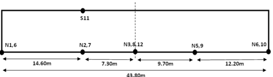
The Dowling Hall footbridge has a total length of 43.80m and a width of 3.20m, with two symmetric spans. The bridge is equipped with a heated deck system in order to avoid the snow accumulation during the winter months.
19
1.2 Instrumentation
The instrumentation employed during the dynamic tests included 12 accelerometers, a data acquisition device and a laptop, which allowed us to measure the bridge’s ambient acceleration response.
PCB Piezotronics 393B04 model accelerometers, which are shown in Figure 1.2, were used to measure the bridge acceleration response. The sensors’ characteristics are shown in Table 1.
Table 1 PCB accelerometers properties
Flexural ICP acceleration 1000 mV/g
Sensitivity ±10%
Broadband resolution (1 to 10000 Hz) 0.000003 g rms
Measurement range ±5 g
Frequency range (±5%) 0.06 to 450 Hz Electrical connector 10-32 coaxial jack
Weight 1.8 oz (50 gm)
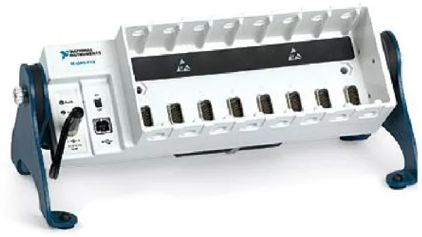
The data acquisition system consisted of two parts: the National Instruments (NI) USB-9234 modules, which are shown on the right side of Figure 1.2 and the National Instruments cDAQ 9172 chassis, which is shown in Figure 1.3.
Figure 1.2 PCB Piezotronics 393B04 accelerometer (left), NI USB-9234 module (right)
20
NI USB-9234 is a 4-Channel, ±5 V, 24-Bit software-selectable IEPE and AC/DC analog input module which provides the accelerometers connection. The NI USB-9234 includes an internal master timebase with a frequency of 13.1072 MHz. The frequency of a master timebase ( fM)
controls the data rate ( fs) of the NI USB-9234. The following Equation (1.1) provides the available device data rates:
256 = M s f f n (1.1)
where n is an integer between 1 and 31. According to Equation (1.1), the acceptable sampling frequency rates are 51.2 kHz, 25.6 kHz, 17.067 kHz, and so on down to 1.652 kHz, depending on the value of n. A manageable 2.048 kHz sampling rate was selected for data acquisition.
21
The NI cDAQ-9172, shown in Figure 1.3, is an eight-slot USB chassis designed for use with I/O modules. The NI cDAQ-9172 chassis is capable of measuring a broad range of analog and digital I/O signals and sensors using a Hi-Speed USB 2.0 interface. Labview Signal Express 3.0 software was used to record the data.
1.3 Dynamic tests performed
1.3.1 April test
On April 4 2009, a set of five dynamic tests were performed on the Dowling Hall footbridge in order to identify its modal parameters (natural frequencies, damping ratios and mode shapes). Figure 1.6 shows the instrumentation employed during the tests.
Twelve accelerometers were placed in different positions on the north and the south sides of the bridge, symmetrically about the centre of the structure as shown in Figure 1.5. The arrangement of sensors has been chosen referring to the mode shapes proposed by the theory of structures dynamic. In order to obtain the measurements for each sensor on at least the first three vibration modes, accelerometers position have been referred to the theoretical framework of the deformation in the dynamic field of a symmetrical beam on three supports, so as to avoid the nodes, where the displacements are zero and therefore the accelerations. Figure 1.4 shows the first two theoretical dynamic deflections for a continuous beam and the sensors locations, selected in order to provide significant results during the dynamic tests.
22
Figure 1.4 Sensors locations showing dynamic deformations
Sensors placement on the structure's deck was preceded by the study of the dynamic characteristics of plates that make up the concrete slab. This analysis is necessary to identify the natural frequencies of concrete elements and avoid the mistake with the results relative to the whole structure. The study was conducted on a plate type, since all elements have the same size and subject to the same degree of restraint. The frequencies were found to be higher than that of the steel structure of the bridge, with the first natural frequency around 16 Hz and higher frequencies greater than 30 Hz. This observation has led to correctly identify the natural frequencies of the bridge without interference by concrete elements.
The accelerometers were set as close as possible to the steel trusses, on the outer sides of the slabs of concrete, so that they do not affect the detection frequencies of the steel structure. Furthermore, the sensors were placed in correspondence of the horizontal steal currents, near the junction with the main structure, to improve the detection of the steal frame frequencies.
In order to provide a tight connection between the sensors and the concrete slabs, aluminum angular brackets were firmly fixed to the concrete deck using a fast-setting two-part epoxy cement. The brackets were machined to accept the mounting stud of the accelerometer. Then, the accelerometers were screwed into the brackets.
23
Figure 1.5 April test sensors layout along the bridge deck
The five tests have been performed by exciting the structure with pedestrian traffic and people jumping in various positions along the bridge deck, together with wind excitation. Two sensors configurations were selected in order to measure both vertical and horizontal components of the bridge acceleration response:
1. The vertical configuration, consisting of all the twelve sensors measuring vertical accelerations
2. The horizontal-vertical configuration, employing the six south side (S) sensors measuring vertical accelerations and the six north side (N) sensors measuring horizontal accelerations. The five tests were performed in succession, using a sampling rate of 2.048 kHz imposed by instrumentation, and an acquisition time of 300 seconds, maximum time allowed by the acquisition software used, resulting in 614,400 samples per channel. A high acquisition time was required to achieve high definition signal in the frequency domain, resulting in the distance between two points in the frequency domain (df) is inversely proportional to the total time of acquisition.
Preparation for the test began on the afternoon of April 3rd with cementing of the steel brackets to the bridge deck. This was done to allow overnight curing of the epoxy and avoid setting up in the rain which was predicted for the following morning.
Final preparations for the test were finished on the morning of June 4th, including installation of all sensors, cable connections, and data acquisition hardware. The actual test was conducted between 12:00 and 14:30. Weather conditions at the time of the test were cloudy and quite raining, with moderate wind and a temperature of 10° to 13° C.
24
The description of the five tests is presented:
1. Test 1 consisted of recording the accelerations of the structure caused by wind and pedestrian excitation, using the vertical accelerometers configuration.
2. During Test 2, the bridge was excited by wind, pedestrian traffic and people jumping in different locations along the bridge deck. The test was performed using vertical accelerometers configuration.
3. Test 3 was conducted in the same excitation conditions as Test 1, still using vertical accelerometers configuration.
4. Test 4 consisted of recording the accelerations of the structure caused by wind and pedestrian excitation, using the vertical-horizontal accelerometers configuration.
5. During Test 5, the bridge was excited by wind, pedestrian traffic and people jumping in different locations along the bridge deck. The test was performed using vertical-horizontal accelerometers configuration.
25 1.3.2 June test
On June 4 2009, a second set of five dynamic tests were performed on the Dowling Hall footbridge, starting from the results of April test.
The objectives of this second test were to: 1) quantify motion at the supporting piers; 2) gather more data on the horizontal motion of the bridge; 3) detect any significant axial motion. Accelerometers were laid out as shown in Figure 1.7.
Figure 1.7 June test sensors layout along the bridge deck
Twelve accelerometers were placed in different positions on the north and the south sides of the bridge. The arrangement of sensors has been chosen in order to provide accelerations at the three supports location. A reference sensor (N5,9) has been placed in the same position of the April test, so that a comparison and calibration of the data from the two tests was possible.
The accelerometers were set as close as possible to the steel trusses, on the outer sides of the slabs of concrete, so that they do not affect the detection frequencies of the steel structure. Furthermore, the sensors were placed in correspondence of the horizontal steal currents, near the junction with the main structure, to improve the detection of the steal frame frequencies.
In order to provide a tight connection between the sensors and the concrete slabs, aluminum angular brackets were firmly fixed to the concrete deck using a fast-setting two-part epoxy cement. The brackets
26
were machined to accept the mounting stud of the accelerometer. Then, the accelerometers were screwed into the brackets.
The five tests have been performed by exciting the structure with pedestrian traffic and people jumping in various positions along the bridge deck, together with wind excitation. Sensors configurations were selected in order to measure both vertical and horizontal components of the bridge acceleration response for all the accelerometers locations. An axial component configuration accelerometer (N12) was places at the center pier. Finally, one accelerometer (S11) was fixed with the vertical configuration on the south side, corresponding to the N2,7 sensors on the north side, in order to get the acceleration at the same horizontal coordinates of the bridge.
The five tests were performed in succession, using a sampling rate of 2.048 kHz imposed by instrumentation, and an acquisition time of 300 seconds, maximum time allowed by the acquisition software used, resulting in 614,400 samples per channel. A high acquisition time was required to achieve high definition signal in the frequency domain, resulting in the distance between two points in the frequency domain (df) is inversely proportional to the total time of acquisition.
Preparation for the test began on the afternoon of June 3rd with cementing of the steel brackets to the bridge deck. This was done to allow overnight curing of the epoxy and avoid setting up in the rain which was predicted for the following morning.
Final preparations for the test were finished on the morning of June 4th, including installation of all sensors, cable connections, and data acquisition hardware. The actual test was conducted between 11:00 and 12:30. Weather conditions at the time of the test were sunny and dry, with low wind and a temperature of 25° to 27° C.
The description of the five tests is presented:
1. Test 1 consisted of recording the accelerations of the structure caused by 3 minutes with five persons running and jumping across the bridge and 2 minutes with no excitation.
2. During Test 2, the bridge was excited by:
1 minute: with five persons jumping at the midpoint between the center pier and Dowling Hall;
27
1 minute: with five persons standing at the midpoint between the center pier and Dowling Hall;
1 minute: five persons moving to the midpoint between the center pier and main campus;
1 minute: five persons jumping at the midpoint between the center pier and main campus;
1 minute: five persons standing at the midpoint between the center pier and main campus;
3. Test 3 was conducted with one person walking/lightly jumping across the bridge for 5 minutes
4. Test 4 consisted of recording the accelerations of the structure caused by:
1 minute: hammer impacts at 8m from center on campus side (vertical hammer)
1 minute: hammer impacts at 8m from center on campus side (horizontal hammer)
1 minute: hammer impacts at 2,5m from center on campus side (vertical hammer)
1 minute: hammer impacts at 5m from center on Dowling Hall side (vertical hammer)
1 minute: hammer impacts at 5m from center on Dowling Hall side (horizontal hammer)
5. During Test 5, the bridge was excited with similar conditions employed performing Test 4, with input data from impact hammer added to record as Channel 13.
28
29
2. ROW
PROCESSING
OF
EXPERIMETAL DATA
Before the system identification methods were applied to the measured data, they were filtered and down-sampled.
The down-sampling process allows decreasing the signal’s number of samples maintaining the original signal quality. The down-sampled signal is obtained by selecting one sample for every N sample in the signal’s time history, where N is the integer number that defines the down-sampling factor. The down-sampling process is performed in order to improve the computational efficiency of data analysis process.
Increasing the integer N, the computation becomes lighter but, at the same time, the sampled signal is less accurate. The down-sampling factor has to be determined based on the frequencies of interest.
The sampling frequency, according to the NI 9234 timebase frequency, was assumed equal to 2048 Hz. The highest identifiable frequency is the Nyquist frequency, equivalent to half the sampling rate used. Given the large number of samples collected during each phase of testing, analysis may be computationally expensive. To make the calculation less demanding, a downsampling was performed on data sampled in the time domain, thus reducing significantly the number of samples that make up the single signal and lowering the sampling frequency to values more compatible with the natural frequencies are seeking.
In fact, the maximum frequency detectable in the frequency domain, corresponding to the Nyquist frequency, is assumed to be: fd ≤
2B , where where fp is the pulse frequency (in pulses per second) and B is the bandwidth (in hertz). The quantity 2B later came to be called the Nyquist rate.
30
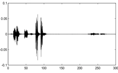
Figure 2.1. Acceleration time history of Channel S2 Test 2
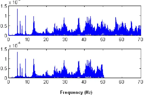
Figure 2.1 shows the acceleration time history at Channel S2 during Test 2, before filtering and down-sampling.
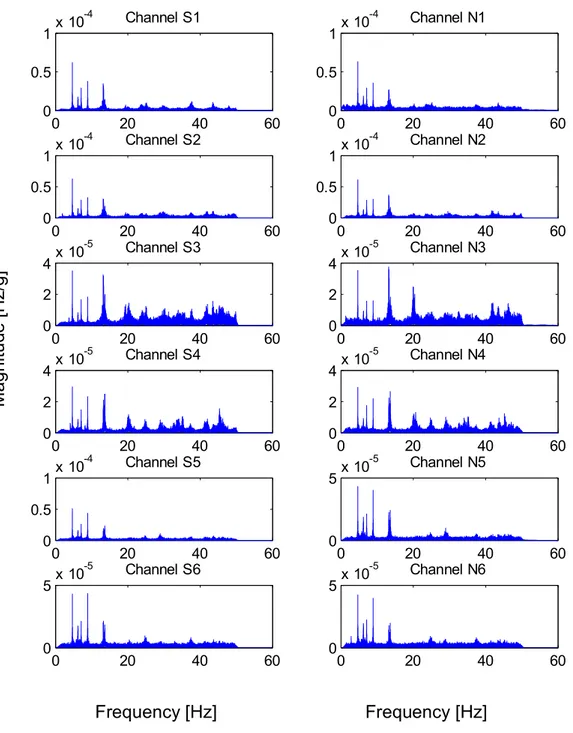
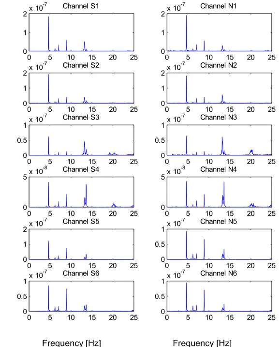
Appendix A presents plots of the time history, Fourier spectra and power spectral density for all the channels and the five tests performed.
2.1 Filtering
Signal filtering is often used in eddy current testing to eliminate unwanted frequencies from the receiver signal. While the correct filter settings can significantly improve the visibility of a defect signal, incorrect settings can distort the signal presentation and even eliminate the defect signal completely. Therefore, it is important to understand the concept of signal filtering.
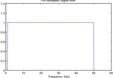
Figure 2.2 shows the finite impulse response (FIR) band-pass digital filter designed and applied for data filtering. The data filtering process allows selecting the frequency range of interest by designing and applying a digital filter. The three standard filters found in most impedance plane display instruments are:
the ‘High Pass Filter (HPF); the‘Low Pass Filter (LPF);
0 50 100 150 200 250 300 -0.1 -0.05 0 0.05 0.1
31
the Band Pass Filter’ (BPF), which is an high and low pass filter combination.
The HPF allows high frequencies to pass and filters out the low frequencies. The HPF is basically filtering out changes in the signal that occur over a significant period of time. The LPF allows low frequency to pass and filters out the high frequency. In other words, all portions of the signal that change rapidly (have a high slope) are filtered, such as electronic noise.
The main function of the LPF is to remove high frequency interference noise. This noise can come from a variety of sources including the instrumentation and/or the probe itself. The noise appears as an unstable dot that produces jagged lines on the display as seen in the signal from a surface notch shown in the left image below. Lowering the LPF frequency will remove more of the higher frequencies from the signal and produce a cleaner signal as shown in the center image below. When using a LPF, it should be set to the highest frequency that produces a usable signal. The HPF is used to eliminate low frequencies which are produced by slow changes, such as conductivity shift within a material, varying distance to an edge while scanning parallel to it, or out-of-round holes in fastener hole inspection. The BPF is typically used to isolate the component of a time series that lies within a particular band of frequencies.
Low-pass or band-pass filters with low frequencies ranges are typically used in studying bridges, which are flexible structures characterized by low natural frequencies. A band-pass digital filter with a 2-50 Hz range has been designed for the Dowling Hall footbridge analysis.
FIR, Finite Impulse Response, filters are one of the primary types of filters used in Digital Signal Processing. FIR filters are said to be finite because they do not have any feedback. Therefore, if you send an impulse through the system (a single spike) then the output will invariably become zero as soon as the impulse runs through the filter.
There are a few terms used to describe the behavior and performance of FIR filter including the following:
Filter Coefficients - The set of constants, also called tap weights, used to multiply against delayed sample values. For an FIR filter,
32
the filter coefficients are, by definition, the impulse response of the filter.
Impulse Response – A filter’s time domain output sequence when the input is an impulse. An impulse is a single unity-valued sample followed and preceded by zero-valued samples. For an FIR filter the impulse response of a FIR filter is the set of filter coefficients. Tap – The number of FIR taps, typically N, tells us a couple things
about the filter. Most importantly it tells us the amount of memory needed, the number of calculations required, and the amount of "filtering" that it can do. Basically, the more taps in a filter results in better stopband attenuation (less of the part we want filtered out), less rippling (less variations in the passband), and steeper rolloff (a shorter transition between the passband and the stopband).
Multiply-Accumulate (MAC) – In the context of FIR Filters, a "MAC" is the operation of multiplying a coefficient by the corresponding delayed data sample and accumulating the result. There is usually one MAC per tap.
Reducing the number of taps used in the filter will reduce the number of calculations to process in the signal, however, the quality of the filtering will suffer. Rippling will become more sever, the rolloff will be less steep, and the passband will be less accurate.
The designed FIR filter is characterized by the 2-50 Hz band-pass range frequencies and by the 4096 N-th order, as shown in Figure 2.2.
Figure 2.2 FIR band-pass digital filter
0 10 20 30 40 50 60 0 0.2 0.4 0.6 0.8 1 1.2 1.4
FIR bandpass digital filter
33
The impulse response, the filter's response to a Kronecker delta input, is finite because it settles to zero in a finite number of sample intervals. This is in contrast to infinite impulse response (IIR) filters, which have internal feedback and may continue to respond indefinitely. The impulse response of an Nth-order FIR filter lasts for N+1 samples and then dies to zero. The FIR digital filter is real and has linear phase.
Figure 2.3 shows the effect of the digital filter on a Fourier amplitude spectrum.
Figure 2.3 Fourier amplitude spectra of Channel S2 during Test 2, before and after filtering
Figure 2.3 shows a Fourier spectrum sample before and after the FIR digital filter application.
2.2 Down-Sampling
The data down-sampling process allows the number of samples reduction in signal’s time history by picking one sample from every N, where N is a real integer usually called sampling factor. The down-sampling factor N is selected such that the down-sampled Nyquist
34
Frequency is still larger than the frequency range of interest. In addition, low-pass filters should be applied to the data before down-sampling in order to avoid aliasing. In this work the down-sampling factor has been selected equal to 8, corresponding to a down-sampled signal eight times smaller than the original one. However, the quality of the “new” signal is still acceptable as shown in Figure 2.4. The down-sampling process allows working with less data without compromising the signal quality.
According with the N value, sampling rate has been reduced from 2.048 kHz to 256 Hz, corresponding to a samples decreasing from 614,400 to 78,600 samples for each channel.
Figure 2.4 Original and the down-sampled signal.
If the sampling condition given by the Nyquist-Shannon sampling theorem is not satisfied, adjacent copies overlap, and it is not possible in general to discern an unambiguous signal. Any frequency component above is indistinguishable from a lower-frequency component, called an alias, associated with one of the copies. Aliasing refers to an effect that causes different signals to become indistinguishable (or aliases of one another) when sampled.
For a sinusoidal component of exactly half the sampling frequency, the component will in general alias to another sinusoid of the same frequency, but with a different phase and amplitude.
16.3 16.31 16.32 16.33 16.34 16.35 -0.02 -0.015 -0.01 -0.005 0 0.005 0.01 0.015 Original Downsampled
35
To prevent or reduce aliasing, two things can be done:
Increase the sampling rate, to above twice some or all of the frequencies that are aliasing.
Introduce an anti-aliasing filter or make the anti-aliasing filter more stringent.
2.3 Fourier transform and Power Spectral Density
Non-sinusoidal periodic signals are made up of many discrete sinusoidal frequency components (see applet Fourier Synthesis of Periodic Waveforms). The process of obtaining the spectrum of frequencies H(f) comprising a time-dependent signal h(t) is called Fourier Analysis and it is realized by the so-called Fourier Transform (FT). A single square pulse or an exponentially decaying sinusoidal signal are typical examples of non-periodic signals, of finite duration. Even these signals are composed of sinusoidal components but not discrete in nature, i.e. the corresponding H(f) is a continuous function of frequency rather than a series of discrete sinusoidal components
The traditional approach to a modal parameters identification process consists of detecting the natural frequencies directly from peaks in the signal’s Fourier amplitude spectra. The signal is generally acquired in time domain (signal time history) and then transformed into its corresponding frequency domain. The Fourier transform (FT) is a widely used mathematical tool to get this transformation.
The periodic signals, i.e. if x (t) = x (t + T0) for each instant of
time t, since T0 is the period, can be written as a sum, usually finite, of harmonic functions through the Fourier series:
( ) jk t k k x t X e
(2.1)where the coefficients Xk are derived from the following expression (2.2):
36
0 0 0 2 2 0 2 1 ( ) d T jk t T k T X x t e t T
(2.2)The Fourier transform is a generalization of the Fourier series to the case where the function x(t) is not periodic (i.e. infinite period). The Fourier transform of a function x(t) is given by the (2.3):
( ) j td k X x t e t
(2.3)To calculate the Fourier coefficient corresponding to the k-th harmony through discrete steps Δt, should approximate formula (2.2) as follows: 2 1 0 1 ( ) N jk n t N t k n X x n t e N t
(2.4)where the summation term is the fast Fourier transform (FFT) or discrete transform. The discrete Transforms produce Fourier spectra consist of values in which each can be thought as the output of a filter centered at frequency ω.
The autocorrelation function for a generic signal x(t) is:
0 1 lim ( ) ( )d T xx T R x t x t t T
(2.5)showing the correlation of a signal to itself. The autocorrelation of a periodic function is periodic, while the autocorrelation of a random signal tends to zero for nonzero τ. The Fourier transform of the autocorrelation function Rxx(τ) is that power spectral density (PSD), or autospettrum,
defined as:
2
j xx xx S R e d (2.5)37
Function Sxx(ω) is related to the Fourier transform X(ω) of x(t) by
report:
xxS X X (2.6)
where X(ω)* indicates the complex conjugate of X(ω). It is a real function and contains information on the frequencies present in x (t) but not those on the phases, as obtained from the only form. X(ω). The cross-correlation (or cross-cross-correlation) function of two signals x(t) and y(t) is defined as:
T T xy x t y t t T R 0 d ) ( ) ( 1 lim (2.7)and indicates how the two signals are correlated. Fourier transform function of cross-correlation Rxy is called cross-spectrum (CSD) and is usually indicated by Sxy(ω):
j2 d xy xy S R e
(2.8)Function Sxy(ω) is related to the Fourier transform of x(t) and y(t) by the
expression:
xyS X Y (2.9)
that is a complex function containing information both on frequencies and phases.
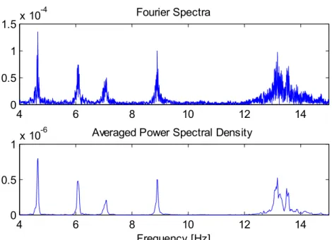
Through the FFT, the frequency domain shows the signal’s frequency content, allowing the direct natural frequencies detection. The signal can also be analyzed into its frequency domain by using the power spectral density (PSD), providing the representation of the frequencies power content. Using PSD, the signal can be averaged through the
38
windowing process in order to provide smoother plots as shown in Figure 2.6
.
Figure 2.5 Fourier spectra and averaged PSD. of Channel S2 during Test 2.
The purpose of the window function is to reduce side-lobe level in the spectral density estimate, at the expense of frequency resolution, exactly as in the case of sinusoidal spectrum analysis.
Welch's method is based on the concept of using periodograms, which converts a signal from the time domain to the frequency domain.
The Welch method develops in the following steps:
The signal is split up into overlapping segments. The original data segment is split up into L data segments of length M, overlapping by D points.
If D = M/2, the overlap is said to be 50% If D = 0, the overlap is said to be 0%.
The overlapping segments are then windowed. After the data is split up into overlapping segments, the individual L data segments have a window applied to them (in the time domain). Most window functions afford more influence to the data at the center of the set than to data at the edges, which represents a loss of information. To mitigate that loss, the individual data sets are commonly overlapped in time (as in the above step).
4 6 8 10 12 14 0 0.5 1 1.5x 10 -4 Fourier Spectra 4 6 8 10 12 14 0 0.5 1x 10
-6 Averaged Power Spectral Density
39
The windowing of the segments is what makes the Welch method a "modified" periodogram.
The periodogram is calculated by computing the discrete Fourier transform, and then computing the squared magnitude of the result. The individual periodograms are then time-averaged, which reduces the variance of the individual power measurements.
A window function is a function that is zero-valued outside of some chosen interval. For instance, a function that is constant inside the interval and zero elsewhere is called a rectangular window, which describes the shape of its graphical representation. When another function or a signal (data) is multiplied by a window function, the product is also zero-valued outside the interval: all that is left is the view through the window.
The generalized Hamming family of windows is constructed by adding one period of a cosine function to the rectangular window. The benefit of adding the cosine segment is lower side lobes. An example of Hamming window representation in time domain is shown in Figure 2.6.
Figure 2.6 Hamming window
In this work the power spectral density has been computed using Welch's method. Windowing is applied by 9600 points (N) Hamming windows with 50% overlap resulting in a frequency resolution of
0.016
f
41
3. MODAL ANALYSIS
System identification using output-only ambient response was originally performed in frequency domain. The method of selecting peaks in frequency domain of spectral density is generally called the Peak Picking method (Bernat & Piersol, 1993) and has been used extensively in classical modal analysis based on ambient excitation. Several techniques were later developed to facilitate an automatic ‘picking’ procedure, such as frequency domain decomposition using singular value decomposition of power spectral density. However, in practice the classical identification techniques that use spectral analysis give reasonable estimates of natural frequencies and mode shapes only if the modes are well separated. Natural Excitation Technique (NExT) (James et al. 1993) combined with Eigensystem Realization Algorithm (ERA) (Juang and Pappa 1985) have been frequently used for modal identification of structures. NExT-ERA has been successfully applied to structural identification based on ambient excitation (He et al. 2009; Farrar and James 1997). In this section the Peak Picking method and the NExT-ERA are briefly reviewed and their modal identification results are presented.
3.1 Peak Picking
Ambient excitation testing does not directly lend itself to FRFs or IRFs calculations because the input forces are not measured. In the paper two modal parameter identification methods that can deal with ambient vibration measurements are implemented. The first is a rather simple Peak-Picking (PP) method. Though it has some theoretical drawbacks,
42
the Peak-Picking method is probably the most widely used method in civil engineering because of its simplicity.
3.1.1 Method
The Peak-Picking method (Bendat and Piersol 1993) is the simplest known method for identifying the modal parameters of civil engineering structures subjected to ambient vibration loading.
The method leads to reliable results provided that the basic assumptions of low damping and well-separated modes are satisfied. In fact, when a lightly damped structure is subjected to a random excitation, the output ASD at any response point (and the CSD amplitude between any two measurement points) will reach a maximum at frequencies where either the excitation spectrum peaks or the frequency response function of the structure peaks. Since narrow-band peaks in the frequency response function of lightly damped mechanical systems occur at the frequencies corresponding to system normal modes (resonance frequencies), peaks in the ASDs and CSDs can be generally assumed to represent either peaks in the excitation spectrum or normal modes of the structure. In order to identify the output spectral peaks which are due to vibration modes, it has to be recalled that all points on a structure responding in a lightly damped normal mode of vibration will be either in phase or 180° out of phase with one another; hence, for well-separated modes, the spectral matrix can be approximated in the neighbourhood of a resonant frequency fr as a rank-one matrix:
(3.1)
where αr is a scale factor depending on the damping ratio, the natural frequency, the modal participation factor and the excitation spectra.
Equation (3.1) highlights that:
1. each row or column of the spectral matrix at a resonant frequency
fr can be considered as an estimate of the mode shape φr at that frequency;
43
2. the square-root of the diagonal terms of the spectral matrix at a resonant frequency fr can be considered as an estimate of the mode shape φr at that frequency.
Figure 3.1 Complex modes representation
The corresponding modal damping ratios can be estimated based on half-power bandwith as shown in Equation (3.2).
2,i 1,i i n,i ω + ω ξ = 2ω (3.2)
where n i, is the i-th natural frequency, 1,i and 2,i are the frequencies corresponding to magnitude of H/ 2, where H is the value of the peak Fourier amplitude spectra at the i-th natural frequency. Identified damping from Equation (3.2) depends on the shape of the Fourier spectrum plot (i.e. the sharper the peak is, the smaller is the structure’s damping).
In the present application of the PP method, natural frequencies were identified from resonant peaks in the ASDs and in the amplitude of CSDs, for which the cross-spectral phases are 0 or π. The mode shapes were obtained from the amplitude of square-root ASD curves while CSD phases were used to determine directions of relative motion. Drawbacks
44
of the PP method (Abdel-Ghaffar and Housner 1978) are related to the difficulties in identifying closely spaced modes and damping ratios.
Figure 3.2 Power Spectra example
In the context of ambient vibration measurements the FRF is only replaced by the auto spectra of the ambient outputs. In such a way the natural frequencies are simply determined from the observation of the peaks on the graphs of the averaged normalized power spectral densities (ANPSDs). The ANPSDs are basically obtained by converting the measured accelerations to the frequency domain by a discrete Fourier transform (DFT).
Although the input forces are not measured in ambient vibration testing, this problem has often been circumvented by adopting a derived modal parameter identification technique where the reference sensor (base station) signal is used as an “input” and the FRFs and coherence functions are computed for each measurement point with respect to this reference sensor. It not only helps in the identification of the resonances, but also yields the operational shapes that are not the mode shapes, but almost always correspond to them. The coherence function computed for two simultaneously recorded output signals has values close to one at the resonance frequencies because of the high signal-to-noise ratio at these frequencies. Consequently inspecting the coherence function may assist
45
to select the frequencies. In current Peak-Picking method, the components of the mode shapes are determined by the values of the transfer functions at the natural frequencies. Note that in the context of ambient testing, transfer function does not mean the ratio of response over input force, but rather the ratio of response measured by a roving sensor over response measured by a reference sensor. So every transfer function yields a mode shape component relative to the reference sensor. Here it is assumed that the dynamic response at resonance is only dominated by one mode. The validity of this assumption increases as the modes are better separated and as the damping in the structure is lower.
The Peak-Picking is a kind of frequency domain based technique. Frequency domain algorithms are most popular, mainly due to their simplicity and processing speed, and also for historical reasons. These algorithms, however, involve averaging temporal information, thus discarding most of their details.
Peak-picking technique has some theoretical drawbacks: • Picking the peaks is always a subjective task;
• Operational deflection shapes are obtained instead of mode shapes; • Only real modes or proportionally damped structures can be
deduced by the method;
• Damping estimates are unreliable.
In spite of these drawbacks many civil engineering cases exist where the eak-picking technique is successfully applied. The popularity of the method is due to its implementation simplicity and its speed.
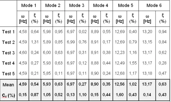
3.1.2 Identification results
Table 3.1 and Table 3.2 present the natural frequencies and the damping ratios of the six identified modes for each of the 4 April and 4 June five tests, respectively. The modes frequencies have been compared using the coefficient of variation (Cv), defined as: Cv=σ/μ. It is a normalized measure of dispersion of a probability distribution. The small coefficient of variation (Cv) for the identified natural frequencies indicates the accuracy of these estimates. However, the same accuracy is not found for the damping ratios. The Cv of the natural frequency estimates are in the range of 0,13-1,6%, while the corresponding
46
coefficient for damping ratios are in the range 0,42-1,09%. However, these identified damping values provide an estimation of the structure’s damping. Table 3.1 put in evidence the accuracy of the system identification method, showing precise results especially for Mode 1 and Mode 3, the first vertical deflection and torsional modes respectively.
Table 3.1 April tests Peak Picking identification results
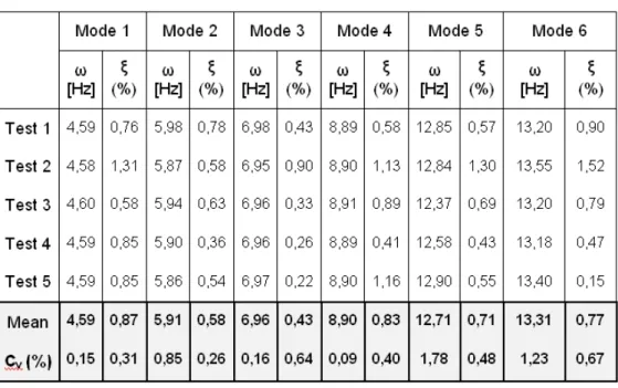
Results from 4 June test are collected in Table 3.2. Data show a good correlation between the six modes identified, with best results for Mode 1 and Mode 3 as the 4 April test results. The influence of the ambient factor can be recognize, in particular the temperature effect on the structure’s stiffness variation. The natural frequencies identified on the 4 June test are smaller than the natural frequencies identified on the 4 April test. This fact is due to a warmer temperature on the June test day that provides a less structure’s stiffness and so smaller natural frequencies. However, both results from the two tests are really close one to the other, showing the good efficiency of the instrumentation and of the system identification process employed.
47
Table 3.2 June tests Peak Picking identification results
Figure 3.2 presents the identified mode shapes corresponding to the six identified modes reported in Table 3.2
48
3.2 Natural Excitation Technique combined with
Eigensystem Realization Algorithm (NExT-ERA)
NExT-ERA is the second method used for system identification of the Dowling Hall footbridge. In the following sections, a brief review of the theoretical bases is provided both for Natural Excitation Technique and Eigensystem Realization Algorithm together with the presentation of system identification result.
3.2.1 Natural Excitation Technique (NExT)
Conventional modal analysis utilizes frequency response functions (FRFs) which require measurements of both input force and the resulting response. However, ambient wind excitation does not lend itself to FRF calculations because the input force cannot be measured. NExT is a four-step process designed to estimate modal parameters of structures excited in their operating environment.
The first step is to acquire response data from the operating structure. Sensors that can measure strain, displacement, velocity, or acceleration response are required. Long time histories of continuous data are desired, provided the operating conditions are relatively stationary.
The second step is to calculate auto- and cross-correlation functions from these time histories using standard techniques. Correlation functions are commonly used to analyze randomly excited systems. As the following section will show, the correlation functions can be expressed as summations of decaying sinusoids. Each decaying sinusoid has a damped natural frequency and damping ratio that is identical to that of a corresponding structural mode.
The third step of NExT uses a time-domain modal identification scheme to estimate the modal parameters by treating the correlation functions as though they were free vibration responses that is, sums of decaying sinusoids. The Eigensystem Realization Algorithm (ERA)
49
have been used as the time-domain modal identification schemes to extract modal frequencies and damping ratios.
The final step of NExT estimates mode shape using the identified modal frequencies and modal damping ratios. An activity closely related to mode shape extraction uses the identified modal parameters to synthesize the auto spectrum from each sensor. This provides a means of visually verifying the accuracy of the estimated modal frequencies and damping ratios.
A theoretical justification of NExT entails proving that a MIMO (multiple input, multiple output), multiple-mode system excited by random inputs produces autocorrelation and cross-correlation functions that are sums of decaying sinusoids.
Furthermore, these decaying sinusoids must have the same damped frequencies and damping ratios as the modes of the system. Consequently, the correlation functions will have the same form as impulse response functions and thus can be used in standard modal analysis algorithms.
The approach is to develop a general solution for a structure with a discrete spatial representation; define the cross-correlation function between two outputs; and solve for the case of random inputs. The theoretical justification of NExT can be developed for a general class of random inputs, fully complex modes, and the presence of known harmonic inputs. However, this development will be limited to the case of white-noise inputs, real modes, and no harmonics, thus allowing the reader to obtain an appreciation for the theoretical background of NExT without the added complexities of the most general case.
The derivation begins by assuming the standard matrix equations of motion:
[M] { x(t)}+ [C] { x(t)}+ [K] { X(t)}= { f(t)} (3.3)
Where:
[M] Is the mass matrix [C] Is the damping matrix [K] Is the stiffness matrix
50
{X} is the vector of random displacements.
Equation (3.3) can be expressed in modal coordinates using a standard modal transformation:
(3.4)
Where:
[Ф] Is the modal matrix
{q(t)} is a vector of modal coordinates {ФT} is the rth mode shape.
A premultiplication of Equation (3.4) by [Ф]T is also performed. Since real normal modes are assumed, [M], [C], and [K] are simultaneously diagonalized. A set of scalar equations in the modal coordinates result:
(3.5)
where:
ωr is the rth modal frequency
ζr is the rth modal damping ratio
mr is the rth modal mass.
The solution of Equation (3.5), assuming a general {f} and zero initial conditions, is obtained from the convolution or Duharnel integral:
(3.6)