1D fluid dynamic modeling of a natural gas light-duty IC engine: predicted results VS measured data

School of Industrial and Information Engineering

Master of science in Energy Engineering – Power Production

1D FLUID DYNAMIC MODELLING OF A

NATURAL GAS LIGHT-DUTY IC ENGINE:

PREDICTED RESULTS vs MEASURED DATA

Supervisor:

Prof. Ing. Angelo ONORATI

Master graduation thesis of:

Luca CASTELLI

Registration number 863557

Quando qualcuno ti chiede: “Chi sei?”

e tu rispondi: “Sono un ingegnere”,

dal punto di vista esistenziale la tua risposta è errata.

Come potresti mai essere un ingegnere?

L’ingegnere è ciò che fai, non è ciò che sei.

Non chiuderti troppo nell’idea della funzione che svolgi

perché vorrebbe dire chiudersi in una prigione.

1

3

Sommario

Lo scopo di questa tesi è stata la creazione e la validazione di un modello termo fluido dinamico per un motore a quattro cilindri in linea alimentato a Gas Naturale, SI, turbocompresso, per veicoli leggeri dedicati al settore dei trasporti. Il motore in analisi, ancora in fase di sviluppo, è l’F1C CNG realizzato da FPT (Fiat Power Train) e testato su un banco prova dedicato presso EMPA – Swiss Federal Laboratories for Materials Science and Technology, che ci fornisce i dati sperimentali necessari per un confronto completo con i risultati delle simulazioni. Inoltre, è stato creato un modello, da parte di EMPA, che utilizza un software commerciale già affermato ed utilizzato di nome GT-Power e da esso è stato possibile estrarre alcune importanti informazioni relative al sistema motore e in particolar modo tutte le dimensioni di ogni componente che deve essere utilizzato durante il processo di costruzione del nostro modello. Altri dati fondamentali per il modello sono stati forniti, in seguito ad alcune richieste di chiarimento, attraverso dei file Excel dedicati.

Il software utilizzato per le simulazioni numeriche è Gasdyn, un codice di calcolo scritto dal gruppo “Internal Combustion Engine” (ICE) del Politecnico di Milano con la collaborazione di Exothermia SA. Esso è accoppiato con una interfaccia grafica (GUI), che, nella sua ultima versione, è chiamata GASDYNPRE3. Attraverso essa lo schema del motore può essere disegnato in tutti i suoi componenti al fine di creare dei file di input necessari per svolgere le simulazioni termo-fluido dinamiche. Alcuni problemi di vario genere sono stati messi in luce durante il periodo di tesi, così da rendere possibile un continuo miglioramento del software.

L’analisi dei risultati delle simulazioni è svolta utilizzando alcuni file Excel creati, gradualmente, durante il periodo di tesi, appositamente per permettere una rapida comprensione degli output ed un confronto esaustivo tra i valori simulati e quelli misurati.

Parole chiavi: 1D CFD, Gasdyn, Motore SI Sovralimentato, Gas Naturale,

5

Abstract

The aim of this thesis has been the creation and validation of a thermo-fluid dynamic model dedicated to a four cylinder in line, turbocharged, light-duty, Spark Ignition, Natural Gas engine dedicated to the truck transportation. The analysed engine, still in the developing phase, is the F1C CNG. It is built by FPT (Fiat Power Train) and it is tested on a dedicated test bench at EMPA – Swiss Federal Laboratories for Materials Science and Technology, which provides the experimental data necessary for a complete comparison procedure with respect to the simulated results. Moreover, this engine is also modelled, by EMPA, using a more affirmed and tested commercial software named GT-Power and from that scheme it is possible to obtain some important informations relative to the engine system and in particular way all the geometric dimensions which have to be used during the building process of our model. Other fundamentals data are provided, after some request of clarifications, through dedicated excel files.

The software used for the calculations is Gasdyn, a computational research code made by the “Internal Combustion Engine” (ICE) group of the “Politecnico di Milano” in cooperation with Exothermia SA. It is coupled with a Graphical User Interface (GUI), that, in its last version, is called GASDYNPRE3. Through it the scheme of the engine is drawn in all its main components to create the input files necessary to perform the thermo-fluid dynamic simulations. Some problems of various kind have been highlighted during the thesis work period and in this way has been possible to continuously adjust and improve the software.

The post processing analysis of the simulation results is carried out with some excel files created, step by step, during the thesis period, specifically to allow a quick comprehension of the outputs and a good and exhaustive comparison between the simulated and measured values.

Keywords: 1D CFD, Gasdyn, Turbocharged SI engine, Natural Gas, Engine

7

Index

1

Governing equations ... 1

1.1 Introduction ... 1

1.2 Governing equations ... 1

1.2.1 Mass conservation equations ... 2

1.2.2 Momentum conservation equation ... 3

1.2.3 Energy conservation equation ... 4

2

Numerical methods and models ... 7

2.1 Shock-Capturing Methods ... 8 2.2 Lax-Wendroff Scheme ... 10 2.3 MacCormack Method ... 13 2.4 Spurious Oscillations ... 14 2.4.1 FCT techniques ... 15 2.4.2 Flux limiters ... 16

2.5 Heat exchange models ... 17

2.5.1 Annand model ... 18

2.5.2 Woschini model ... 18

3

1D Gasdyn Model ... 20

3.1 Real engine data ... 21

3.2 GT-Power scheme from EMPA ... 22

3.3 Cylinders ... 24 3.4 Valves ... 25 3.5 Turbocharger ... 28 3.5.1 Compressor map ... 29 3.5.2 Turbine map ... 33 3.5.3 Turbocharger matching ... 34 3.6 Intercooler ... 37 3.7 Throttle valve ... 39

viii

3.8 Injection ... 40

3.9 Gasdyn scheme ... 41

3.9.1 Processing of the results ... 44

4

Full load engine results ... 45

4.1 Experimental data ... 45 4.2 Transducer position ... 47 4.3 Model validation ... 49 4.3.1 Performances ... 49 4.3.2 Cylinder pressure ... 56 4.3.3 Injection check ... 60

4.3.4 Turbocharger convergence criteria and shaft velocity ... 63

4.3.5 Intake pressure waves... 69

4.3.6 Exhaust pressure waves ... 71

4.3.7 Wave effect ... 74

4.3.8 Ram effect ... 82

5

Conclusions ... 84

5.1 Future engine improvements... 84

5.2 Possible model developments ... 85

9

Introduction

Nowadays the world of the transportations is searching to new types of sources for the automotive vehicle and in particular for heavy and light-duty trucks. Over the traditional engines, Gasoline and Diesel, and electric vehicles (full electric, hybrid), the natural gas engine are more and more adopted in these years, due to the big availability of the fuel, good pollutants emissions and presence of a wide and consolidated distribution grid already built.

The internal combustion engine operates in very different conditions and so it is important to analyze the engine performances in a lot of rotational speeds and at different loads, to simulate a lot of real operating points. The study of the fluid-dynamic processes in internal combustion engines is particularly challenging due to cyclic substitution of the charge inside the cylinders, which makes the phenomenon strongly unstable both in the intake and exhaust systems. In the past, research activities were based only on experimentation in laboratories through test bench, even if this methodology was onerous in terms of costs and time. Thanks to the numerical codes, it is now possible to create models that are able to simulate the behaviour of an engine, thus reducing the use of experimental campaigns. The 1D and multi-D approaches allow to predict different quantities that are not easily measurable through the experiments and to understand which variables have a greater influence on the different phenomena. Also the pollutants emissions can be predicted by using Gasdyn, and this is a key point nowadays, due to the environmental limits imposed by different countries on the new engines. A big distinction has to be made between 1D and 3D simulation approaches. At the beginning has to be clarified the purpose of the simulation, because if we are interested to study in depth a single process or a certain engine zone it is preferable to use a complex and onerous, but precise 3D model. On the other hand, if the target is to model the entire engine to evaluate performances and global parameters, a 1D model is adopted. Obviously, it is not possible to pretend a high accuracy level in certain complex processes due time and cost reason. In relation to our target we use a 1D computational code (Gasdyn).

The thesis work is divided into 5 chapters:

1st _{In the first chapter, a review of the governing equations of the fluid motion in a} duct is provided under some assumptions, which make faster and easier the computational processes. Conservations equations are obtained and then a vectorization process produce a system written in a matrix form which in required by the numerical methods explained in the next chapter.

x

2nd _{In the second chapter, the numerical methods and models implemented in} Gasdyn are explained. Starting from the Method of Characteristics subsequently two second order, space centered, finite differences methods are introduced: Lax-Wendroff and MacCormack methods. They are shock capturing methods which can find discontinuities in spatial and temporal domain, but obviously being second order accurate generates spurious oscillations according to the Godunov theorem, that can be eliminated with soma techniques. Then the Heat transfer models are presented.

3rd _{In the third chapter the engine, all its parts and the equipments used, are} introduced and analyzed one by one in order to obtain the values required by Gasdyn as input. Starting from the real engine characteristics and using the GT-Power engine scheme as guide line has been possible to create a reliable model which faithfully represent the real operating points. A complete engine Gasdyn model is presented and so the simulations can start.

4th _{In the fourth chapter an initial study of the available measured data, provided} by the EMPA test bench, is made and subsequently the transducers positions are decided, in order to obtain comparable simulated results. The simulation outputs are analyzed and collated with the experimental data in order to validate the engine Gasdyn model. In addition to the performances also other parameters and phenomena are analyzed such as: turbocharger functioning, air mass flow rate and fuel injection, cylinder pressure, ram and waves effects. 5th _{In the last one the conclusions are summarized and some possible}

improvements both on the engine model and also on the real motor are proposed and illustrated. Moreover, the future Gasdyn model developments have been briefly introduced for the next student which will be interested by this type of thesis work.

1

1 Governing equations

1.1 Introduction

Internal combustion engine is classified as reciprocating fluid-dynamic machine, characterized by a non-stationary fluid motion due to the engine cyclic behaviour (steady-state hypothesis is not valid). In the intake and exhaust engine ducts the moving gas can be defined as:

- Unsteady - Compressible - Viscous - 3-Dimensional

- Heat fluxes across wall

- High temperatures and pressure gradients - High Reynold’s numbers

Numerical simulation of this kind of machine has to be done with appropriate numerical codes that take in to account the complexity of the system and can correctly reconstruct pressure waves in the engine ducts. Using a DNS methods which study Navier-Stokes equations in the 3D domain, it is possible to achieve quite precise outcomes, but the computational complexity and the time expenditure is too much in relation to the accuracy obtainable using faster approaches.

1.2 Governing equations

To study an internal combustion engine is more adequate to rewrite the N-S equations under a 1 D point of view and introducing some approximations, obtaining others governing equations which define in a good way the gas motion in the ducts. In this way we are able to simplify the system and use faster computational approaches, keep accuracy above a certain reasonable limit and drastically reduce the necessary amount of time.

Governing equations

2

- Unsteady gas flow

- 1-D motion inside the engine ducts. The directions different from the curvilinear abscissa are negligible

- Compressible flow - Non-adiabatic process

- Non-isentropic process (Inviscid fluid) - Heat fluxes and friction exist only at the wall - Negligible variation of the duct section

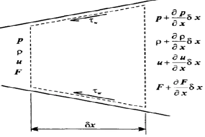
Applying an Eulerian approach and considering the previous assumptions I can consider this control volume and analyze these quantities:

Figure 1: Duct control volume for balance equations

1.2.1 Mass conservation equations

The net rate of change of mass within the control volume, has to be equal to the mass flow rate variation between the inlet and the outlet. Considering F, the variable cross-sectional area, it is possible to write the continuity equation:

Making some reasonable simplifications and neglecting the infinitesimals of the second and higher order we can rewrite the continuity equations as:

3

1.2.2 Momentum conservation equation

The variation, during the time unit, of the momentum of the mass contained into the volume to which we add its net flow, must coincide with the sum of the pressure and shear forces acting on the surface of the control volume. The resulting force on the control volume is given by the pressure differential between the terminal sections and components along x of the pressure acting on the lateral surface of the volume.

The various components can be divided into:

- the contribution of pressure field in x-direction is represented by:

The first two terms take into account the whole pressure on the boundary sections, since the curvilinear abscissa of pipe parallel to the normal versor of pressure. The third term represent force in x-direction produces by the pressure on the sides of control volume.

- The shear force on the control volume is due to the friction between moving fluid and the surface of the duct. Starting from shear stress definition it is possible to write the equation for the friction force on the lateral surfaces:

Usually in 1-D model of internal combustion engine this term is the only that include the fluid viscosity and the character of the governing equation remains essentially inviscid.

The rate of change of momentum within the volume is expressed as follows:

The net flux of momentum through the control volume, is:

So, the whole momentum conservation equation becomes:

Governing equations

4

The equation can be rewritten as:

1.2.3 Energy conservation equation

The energy equation can be derived by applying the First Law of Thermodynamics to the control volume:

The first term represents the variation in time of the total stagnation internal energy, while the second term represents the net flux of enthalpy through the control surface. The summation of these two contributes is equal to the difference of heat entering the system and mechanical work exiting the system.

The two terms at the left-hand side can be rewritten using the specific stagnation quantity:

The work exchanged in the intake and exhaust ducts is null and the energy equation can be rewritten:

For the gases, in an internal combustion engine manifolds and cylinders, it is usually sufficiently accurate a perfect gas with constant specific heat state equation; this refers to a gas that respects the ideal gas state equation and has an internal energy defined as the product of the specific heat at constant volume and the actual temperature. These properties are translated in these relationships:

5

The energy equation can be written eliminating the specific internal energy:

1.16 From the expansion of equation, combined with the conservation of mass equation and with momentum equation the non-conservative formulation of the equation of energy is reached:

The hyperbolic system of governing equations is in the non-conservative form and it is:

The system is now written in a form suitable for the resolution with the Method of Characteristics.

The evolution of CFD and the need to capture in a accurate way all the phenomena that characterise the fluid flow has led to a conservative formulation of the non-linear hyperbolic system. This formulation, solved with Shock-Capturing numerical methods, allows to take into account and describe in a correct way possible discontinuity in the studied flow. The system written in strong conservative form is:

Governing equations

6

To apply the Shock Capturing numerical method, the system is rewritten as a matrix, identifying four vectors:

 Vector of conserved independent variables, whose fluxes remain unchanged through the shockwaves:

 Vector of conserved variables fluxes:

 Vector of the source terms due to pressure force derived from the pipe cross sectional change:

 Vector of source terms related to the fluid friction and heat transfer:

The system, rewritten in the matrix form, will look as follows:

The problem has still three equations and four unknowns; so, to be solved, it is necessary to introduce a relationship that describes the gas behaviour. As done above, it is possible to apply the simplifying hypothesis of perfect gas at specific constant temperatures or adopt a more generic model describing a mix of ideal gasses.

7

2 Numerical methods and models

It is not usually possible to determine an analytical solution of the partial differential hyperbolic system described above. It is necessary to discretize the governing equations to form an algebraic set of relationships that can be solved with the use of a computer. Historically, the first step to find the solution of similar problems was made by Riemann when he developed the Methodology of Characteristics, introducing new computational perspectives, that brought to new numerical methods. The approach is quasi-linear in determining fundamentals between two nodes of the mesh. The main limitations of this method are substantially three:

- Assumption of the perfect gas at specific constant temperatures

- Linear approximation: the space-time domain has been meshed by a calculation grid on the plain (x, t) and the solution is determined between subsequent nodes with accuracy to the first order

- Discontinuity in the solution: the method is not capable to properly detect possible discontinuities in the resolution, as the typical case of shock waves, distributing the phenomenon over the several nodes of the calculation grid. Hence, besides the Method of Characteristics, that remains the most diffused one (because of its simplicity and its physical approach to solve the hyperbolic problem), there are other computational techniques: the shock-capturing finite difference methods. The ability of these techniques is to get the possible shock waves automatically, without the knowledge of the discontinuity position.

There are two groups of these methods. In the first one, “upwind” methods are classified, or “characteristic based”, that give the best results in terms of discontinuity resolution, with high computational burden, since they solve the Riemann problem in each mesh. In the second group, there are the “non-upwinded” methods, also called symmetrical or centered, that apply in each node the same scheme of finite difference, to express partial derivative terms. The Lax-Wendroff, MacCormack and Conservation Element - Solution Element methods enter this class.

Shock-Capturing Methods

8

2.1 Shock-Capturing Methods

The main advantage of the Shock capturing methods is to correctly perceive possible discontinuities in the solution, such as: shock waves, contact discontinuity due to temperature or chemical composition. Within this family the symmetrical finite differentials methods resulted as the most efficient, representing a good compromise between: accuracy, validity of solution, simplicity and length of calculation. The symmetry of the method consists in applying at each node of the grid the same finite differentials scheme to express the terms of the space derivatives, independently from the type of the flow field. The following methods are explicit and have a 2nd order accuracy in the space-time domain. Unfortunately, as it is known from Godunov’s Theorem, accuracy of a higher order than the first leads to spurious oscillations problems in the solution; so, it is necessary the use of particular algorithms in order to mitigate this effect.

Previously, we have seen all the passages bringing to the definition of the vector W(x,t), that allows us to characterize completely the motion of the compressible fluid. Now this vector is considered under the hypothesis of constant cross-sectional area and becomes:

In order to proceed in the numerical modelling, we have to substitute the vector W(x, t) with the equivalent , approximation to , where the subscript i defines the spatial coordinate, while the apex n indicates the considered instant of time. In this way, we obtain a computational grid, characterized by the steps Δx and Δt.

9 Shock-Capturing methods are applied to the hyperbolic system written in conservative and matrix form, with the additional hypothesis about the evolving gas model. Referring to equation 1.24 and deleting the source term vectors, it is possible to obtain Euler Equations, which describe a homentropic flow:

Integrating and applying the Gauss Divergence theorem:

A discretization process of the space-time domain is necessary to apply the finite differences methods. The vector becomes:

Introducing that in the integral:

Where the terms W and F are obtained by making the average in the space and time of the relative vectors:

Equation 2.3 permits to disengage from the condition of derivability, requested by the Euler Equations, even in the presence of discontinuity, furthermore integral formulation has the advantage of treating discontinuities even without prior knowledge of their location. Rearranging properly the terms of equation 2.4 we can write:

By summing the differences along x is obtained:

Lax-Wendroff Scheme

10 In detail:

• the first term on the left-hand side represents the total mass, momentum and energy at time level n + 1.

• the first term on the right-hand side represents the total mass, momentum and energy at time level n

• the second term on the right-hand side represents the flux of conserved quantities through the pipe ends.

The equations so defined, represent a conservative discretization scheme, which guarantees the preservation of integral property of the governing equations.

In the following steps, the Lax Wendroff and MacCormack Shock-Capturing methods will be introduced, both used in Gasdyn and belonging to the finite differentials methods, non-upwind, explicit and with an accuracy of the II° order.

2.2 Lax-Wendroff Scheme

This scheme is based on Taylor series expansions of solution vector W(x,t) and it is developed in two variants: one-step scheme, two step scheme. The version one-step effort requires the calculation of a Jacobian matrix A in each node for all time steps of the simulation, so requires a high computational. The two-step scheme instead removed the need to calculate the Jacobian matrix, while retaining second-order accuracy, by solving the equations in a two-step procedure, inserting an intermediate step in the calculation of the solution vector in the node and at the desired time.

1 Step Scheme

Let's now consider Taylor's series expansion of the state vector in the discretized domain at time n+1 and at node i:

11 The Jacobian Matrix A [3x3] is composed of elements defined by:

The equation 2.2 becomes:

The spatial differences can be approximated by central differences and the series is truncated at second-order terms, giving:

Terms in the square brackets can be discretized as:

So, the Lax-Wendroff equation becomes:

2.16 The Jacobian matrix can be evaluated as:

Due to the necessity of calculating the Jacobian Matrix at each step, the single step Lax Wendroff method ends up being very resource intensive.

2 Step Scheme

Such method avoids calculating the Jacobian matrix, introducing an intermediate step into the calculation of the solution vector, and therefore it is particularly suited for implementing the calculation codes.

 The 1st _{step is based on space-centered differences. Knowing vectors W and F at} nodes i-1, i+1 and at time n, we obtain solution vector W, using a Taylor's series expansion halted at the first order, at intermediate time n+1/2 in intermediate nodes i+1/2. Introducing the approximation at the finite centred differentials, we obtain:

Lax-Wendroff Scheme 12

 2nd _{step: calculate flow vector F at intermediate time n+1/2 in intermediate} nodes i+1/2 and i-1/2, after which it is possible to determine solution vector W at time n in node i:

The general case of non homentropic flow is expressed by introducing the appropriate discretized source terms:

We remind that, in order to establish the dimension of the temporal step, it is used the Courant-Friedrichs-Lewy stability criterion, according to which the max temporal step is equal to:

with , u and a taken from the node, where their sum is maximum.

13

2.3 MacCormack Method

The MacCormack method is another second-order accurate scheme that becomes identical to the Lax-Wendroff scheme for the linear case. The scheme uses alternative forward and backward spatial differences for the two steps in space. Consider the system of equations in conservative and matricial form, with the hypothesis of homentropic flux and constant cross-section duct.

 Predictor step: once the vectors and are known in each node at time n, applying forward differencing, the value of the solution vector * is evaluated at time t*:

interval of :

Forward discretization in space used in the first step is unstable when all the eigenvalues of the Jacobian matrix, A, are positive, and this indicates that the flow is supersonic. The backward discretization in space is unstable for negative eigenvalues, but the overall scheme is stable and has second-order accuracy because the truncation errors for each step cancel out. The following scheme represents the two phases of the MacCormack method:

Spurious Oscillations

14

The stability of the scheme in the case of discontinuities is influenced by the direction of the spatial differencing used in each of the steps. The “forward predictor/backward corrector” arrangement is best suited for discontinuities traveling from left to right, while the opposite is true for the “backward predictor/forward” corrector scheme. Since the propagation of discontinuities is usually not known at any instant, it is usual to reverse the order of spatial differencing at each time step.

Also for this method, the stability condition derives from the application of the CFL criterion:

2.4 Spurious Oscillations

The two methods exposed above are affected by spurious oscillations when the solution is close to a discontinuity (like shock waves and contact discontinuity). This is related to the Godunov’s theorem, which demonstrate that if a numerical solution method is higher than first order of accuracy introduces not-physic oscillations in the solution. Some criterion is required to establish if schemes suffer or not from spurious oscillation. A very tested criterion is the total variation diminishing (TVD) principle. The total variation of solution at the time n is defined by:

If the total variation of the solution doesn’t increase from one-time step to the next one the data are said to be total variation diminishing and so the considered numerical scheme will not produce spurious oscillations at discontinuities.

15 There are essentially two classes of numerical methods for achieving the total variation diminishing condition with high order accuracy:

- Pre-processing schemes: characterized by the fact that the totality of data is modified before updating the solution.

- Post-processing schemes: the solution is updated each time using the chosen numerical scheme and subsequently modified to fulfil the prerequisites of TVD schemes. In this group we find FCT techniques and the flux limiters, which are implemented in the Gasdyn code.

2.4.1 FCT techniques

It uses a high order difference scheme for the initial stage, allowing spurious oscillations to appear, and subsequently applies a global diffusion process to eliminate them. A limited anti-diffusive flux is then applied in order to restore the accuracy of the initial high order stage.

Thus, the general approach consists of three distinct stages:

 Transport stage: first attempt solution is obtained by two-step Lax-Wendroff or

MacCormack methods.

 Diffusion stage: The purpose is to eliminate any spurious oscillation

introduced by the linear second-order transport scheme. A diffusive flux , is calculated as:

For which can be defined the diffusion operator:

There are two possibilities for the diffusion operation:

- Diffusion via damping:

- Diffusion via smoothing:

Spurious Oscillations

16

 Counter-diffusion stage: we introduce the non-linear counter-diffusion agent

A which removes, where not necessary, the diffusion introduced in a uniform way during the preceding phase. A is given by:

2.35

Where ψ, called flux limiter, is defined as by Ikeda and Nakagawa. The final solution can be calculated by:

(a) Damping case:

(b) Smoothing case:

The Smoothing algorithm though is stable but is not able to delete all the spurious oscillations.

2.4.2 Flux limiters

The general philosophy behind Flux Limiters is into the application of an anti-diffusive flow, only in the areas interested by discontinuities, this way we can prevent possible non-physical numeric oscillations. It can be shown that the Lax-Wendroff scheme for the linear advection equation, with a > 0, can be rewritten in the form:

Van Leer introduced parameter , called flux limiter, able to control the numeric oscillations of the solution. This parameter monitors the smoothness of the data and it is a function of the ratio of consecutive solutions gradients and it is defined as:

17 Where:

So, the scheme becomes:

The functionality principle of the algorithms for the application of the flux limiters is based on the following concept: when solutions of adjacent points are similar we maintain the accuracy of the II° order in the numeric method used, whereas in the presence of a discontinuity the accuracy of the method is degraded to the I° order to avoid the spurious oscillations problem.

2.5 Heat exchange models

In the Gasdyn code are present two heat exchange models which compute the net power exchanged between gases and walls. Numerical models that are used to study the evolution of the fluid in the cylinder needs a thermal sub-model able to calculate the instantaneous heat flux between the fluid in the chamber and the walls. The main processes that occurs during the heat transfer are:

 Thermal convection: It represent the main contribute of the total amount exchanged, and it is computed as:

 Thermal radiation: This amount is described by the Stefan Boltzmann law:

where is the Black-body radiation coefficient, ε is emissivity factor, and are the temperatures of the hot gas and the walls. In the cylinder exhaust gas mixture, after combustion completion, only water and carbon dioxide molecules are able to radiate a significant amount of energy, their radiated energy is estimated in a 1% - 2% of total radiated energy on an entire cycle, exhaust product gas radiation is consequently negligible.

Heat exchange models

18

2.5.1 Annand model

Both the convective and the radiative contributes are taken into account using experimental coefficients. The instantaneous and space averaged exchanged heat flux results:

The convective coefficient is related to physic characteristic and cinematic conditions of the gas:

With: - is the averaged piston velocity - D is the cylinder bore

-

-

-

2.5.2 Woschini model

This model neglects the radiative heat flux component, which is considered by overestimating convective contribution. The governing equation of this model is:

Where represent the convective and radiative contributes, and is defined according the following physic relation:

2.49

All variables used in the Woschini model are assumed as functions of the gas temperature:

19 An important parameter, which has to be well defined and calculated, is the reference velocity which includes a contribute related to the density variation during combustion and to the gas exchange process:

With:

Heat exchange models

20

3 1D Gasdyn Model

In the present chapter, with particular attention, we will describe the procedure followed for the modelling of the engine developed in Gasdyn, a simulation software internally developed at Energy department of “Politecnico di Milano”, and more in detail by ICE Group and Exothermia SA. It is a 1D computational thermo-fluid dynamics code, able to simulate the operating conditions of an internal combustion engines, providing an important aid in the setting procedure of each part in order to optimize the interest’s parameters such as torque, power, fuel consumption, noise and emissions, providing also the possibility to predict the gas pressure and temperature in each point of the system.

An internal combustion engine is a complex cyclical machine characterized by an important non-stationariness. Starting from the piston movements until pressure and mass flow variations, a relevant oscillation around an average value is present. Moreover, some gas behaviours are quite difficult to analyse and simulate due to the strong turbulence or complex reactions which occur. Some examples are combustion and gas exchange processes. In these cases, an accurate 3D model would be necessary to simulate with precision how the gas (air, fuel and their mixture) properties evolve in time and space. Obviously, the time expenditure and computational power required by the software to analyse one of these processes, in a certain fixed condition, is largely more onerous with respect to that one necessary for a 1D simulation.

Gasdyn works with a simplified computational code which analyse the situations mentioned above exploiting some models based on reasonable assumptions and approximations, obtaining reliable results quite closed to the experimental results and also to the 3D simulation outputs.

This type of analysis is a key point during the engine design procedure, because allow to study the intake and exhaust processes, which strongly influence the overall efficiency, but also to dimension all the other mechanicals parts which constitute the engine system. The waves and ram effects can be estimated with good accuracy and

21 continuously improved step by step, exploiting an easy 1D approach, saving time and money. Another advantage is the knowledge of the operating condition (temperature and pressure) of each pipe, which facilitate the material choice and dimensioning. In the past decades these analyses were carried out through a lot of tests at some significant rotating speeds and loads, made on the real engine, with the purpose to try as better as possible the real conditions in which the engine works.

3.1 Real engine data

The engine under investigation is the F1C CNG, produced by FPT, and it is intended to equip a light duty vehicle, which need to achieve high values of torque, rather than high peaks of power, for drivability reasons. The version fed with natural gas is obviously derived from its precursor, the Diesel engine, from which the analyzed engine get the main structure and a lot of mechanical parts. An exclusive design would be too expensive, without having a relevant improvement of performances and costs.

GT-Power scheme from EMPA

22

Some technical data:

Table 1: Engine's technical data

3.2 GT-Power scheme from EMPA

The F1C CNG Engine is actually studied and tested at EMPA – Swiss Federal Laboratories for Materials Science and Technology, with which “Politecnico di Milano” cooperate since few years. It provides the engine scheme used in GT-Power simulations, a validated software used for the modelling process and also experimental data measured from own test bench, useful during our validation process. All data related to the engine structure and setting of others mechanical parts are provided through a big text file, which contain the main part of the necessary values referred to all engine’s component, and where necessary it is explained in deep with some additional excel files. Others necessary data, initially missing or encrypted, have been provided after a request of clarification to EMPA on some values which GT-Power sees as default and so cannot be extracted by the text file. In some rare particular situations, no data was available and so some realistic values which produce the attended results has been found through a trial and error procedure.

In the Figure 6 the engine scheme used by EMPA into the GT-Power for the simulations is printed.

Engine name F1C CNG

Cycle Otto cycle – 4 Stroke

Turbocharged with Intercooler Fuel Methane gas

Injection Multiple point – Port Fuel Injection Structure 4 Cylinders in line

4 Valves per cylinder Combustion chamber shape Cylindrical

23

Cylinders

24

3.3 Cylinders

Dimensioning of the combustion chamber and definition of the combustion process parameters has a fundamental importance into the model building procedure. They are responsible for the conversion of the chemical energy into thermal one and finally into mechanical power. The reactions which occur, heavily influence pressure and temperature both in the cylinder and in the exhaust manifold, and so obviously also the performances can be modified. Geometry and combustion have effects on the entire engine operating point and, indirectly, also on the intake side, by changing the rotational speed of the turbocharger shaft, and consequently changing the delivery pressure.

Unfortunately, the combustion process cannot be detailed studied using a 1D approach, but a more complex 3D model is required. This because chemical reactions, air-fuel mixing process and turbulence flow are very difficult to simulate, and the time and computational power required are quite heavy in comparison to our logic. Gasdyn has the purpose to predict pressure, heat release and some pollutants concentration exploiting an easy and fast engine model and so an simplified combustion model is chosen (usually zero-dimensional).

The cylinder geometry has already been defined few pages above during the real engine characteristic presentation and the values used into the simulations are obviously the same. Regarding to the combustion parameters assumed, the combination reported in the Errore. L'origine riferimento non è stata trovata. is chosen at the beginning with the purpose to fit better as possible the measured cylinder pressure curve with respect to the crank angle for the whole engine speed range.

25 During the thesis work has been necessary to vary these values, keeping the starting point as reference, otherwise could not be possible to reach a good combustion process using a unique set of parameters for the whole engine speed range. The first step is represented by the research of the parameters which mainly influence the in-cylinder pressure and temperature. After that a dedicated setting procedure for each regime is necessary to find the final combination of combustion parameters.

3.4 Valves

A right representation of the valve train is a key point of the model building process, because they play an important role in the engine performances which are strongly affected by the gas exchange process. It influences both the combustion, through a more or less efficient scavenging process, and the turbocharger functioning. Intake and exhaust valves are complex equipments which moves unsteadily and so must be well designed, taking into account also the strong accelerations that they have to support. Dimensioning and motion control are key concepts to promote the cylinder gas exchange process and so also the global engine performance. It is necessary to examine both direct and reverse gas flow, in order to calculate the discharge coefficients and consequently the effective flow areas.

In the ideal cycles, valves open and close instantaneously at piston dead center. In practice, they open and close in finite time (to maintain acceptable accelerations and velocities) and often quite far from the piston dead center, for fluid and/or thermo-dynamic reasons.

Each cylinder uses 2 valves to introduce fresh charge and others 2 to discharge the exhaust gases. The valves constitutive parameters as diameter, EVO, IVO, clearance and others cannot be written due to confidentiality reasons.

Flow discharge coefficients are calculated experimentally both for the intake and exhaust valves, and obviously the worst flow condition coincide with the second one. The available data coming from EMPA are expressed in a different scale with respect to the format required as input for Gasdyn and so they have to be rearranged. The measured values start from 0,9 when the lift is null and decrease during the valve opening period and are referred to the valve seat area which is always constant. On the other hand, the values required as input by Gasdyn have to be expressed starting from 0 when the valve is closed and increasing with the lift during the opening period; In this case the reference area is the curtain one which clearly vary. So, to pass from the first to the second reference system, it is necessary to divide by the valve seat area and multiply for the curtain area.

Valves

26

The rearranged discharge coefficients are plotted in the Figure 8.

Figure 8: Direct and Inverse flow discharge coefficient

Valve lifts are provided by EMPA, and looking at the Figure 9 it is possible to note that the lower flow discharge coefficient and seat area of the exhaust valve is partially compensated by a greater lift.

Figure 9: Intake and Exhaust valve lift

So, combining valve lifts and discharge coefficients, the effective flow area for exhaust (inverse) and intake (direct) valves can be computed and plotted in Figure 10.

F low d isc h ar ge coe ff ici en t [-] L/D Direct Inverse L if t [mm ]

Cam shaft degree Intake valve lift Exhaust valve lift

27

Figure 10: Intake and Exhaust effective flow area

Since the data shown above, the overlap period is obviously present and can be plotted both for cams and valves. The significant difference between the 2 overlap periods is due to the clearance which is not null due to space present between the cam and the head valve. E ff . F low a re a [mm 2]

Cam shaft degree Intake effective area Exhaust effective area

Turbocharger

28

This phenomenon is fundamental to have a good gas exchange process exploiting the ram and waves effects which make the gas motions possible, also at crank angle degrees characterized by an opposite motion between piston and gas motion direction. The overlap period allows also to promote the scavenging process: the introduced fresh charge push out the burned exhaust gases.

At the moment a fixed valve timing system is used, but also the variable timing techniques might be applied, with the purpose of optimize the ram and waves effects at different engine speed.

3.5 Turbocharger

During the past decade, turbocharging has become the dominant trend in the automotive engine design, due to the large number of advantages with respect to the negligible drawbacks. It has been thought initially to boost up engine performances (Torque and Power) keeping unchanged all the other parts, but the global engine size reduction which includes lower costs,

weight, space required and a fuel consumption reduction are the main reasons that have promoted the turbocharger use in the last years. Obviously, the required torque and power levels are achieved to guarantee a good drivability, but with a general saving in terms of pollution and costs. This goal can be reached by an increasing of the fresh charge density, exploiting a compression and a usual following cooling processes.

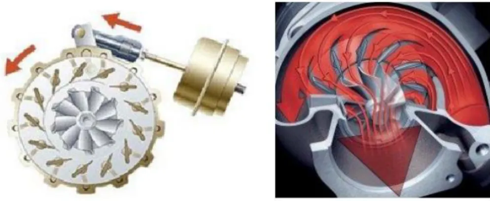
The F1C CNG uses a Mitsubishi TD04HL-F6.0 turbocharger group, composed of a fixed geometry radial turbine and compressor splined on the same shaft, characterized by a pulse system arrangement. Pulse system turbochargers are an evolution of the constant pressure systems, that tries to exploit the high kinetic energy contained in the exhaust gases without transform it in pressure energy. It is possible using narrow pipes which directly connect the exhaust port with the turbine enter section. In this way turbine works with lower efficiency due to the wide flow oscillations, but with an increased available enthalpy drop which produce a greater amount of energy recovered and transmitted to the compressor shaft.

With careful choice of cylinders exhaust ducts grouping in a common duct, combined with a good exhaust pipes design, it is possible to obtain reasonably high turbine

29 operating efficiencies (although rarely as high as values of the constant pressure system). This is particularly critical in a 4-cylinder engine like the F1C where the distance between pressure peaks is 180 CAD. It is inevitable the presence of a certain degree of interference between cylinder exhaust phases, but a multiple turbine entry could be even worse due to the too wide period between consecutive pressure peaks (360 CAD).

To describe the turbocharger behaviour, it is necessary to define characteristics curves both for the compressor and for the turbine, functions of parameters which can be calculated depending on the real operating condition. In this way, it is possible to handle turbocharger with different sizes, using the same process exploiting the similarity theory. All calculations use values expressed in the S.I. system.

3.5.1 Compressor map

The compressor characteristic curve can be drawn with the following parameters defined as: 

All these values are calculated at each speed parameter value, defined as:

Speed parameter

3.4

Turbocharger

30

The turbocharger manufacturer provides the compressor map curves function of these parameters, expressed in a reference system which is different from that one necessary as Gasdyn input and so some calculations are required. Each curve is referred to a speed parameter and can be used, with the others, to predict the shaft behaviour, and as consequence the engine operating points.

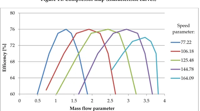
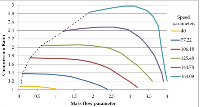
Figure 14: Compressor map (characteristic curves)

Figure 15: Compressor efficiency map

1 1.2 1.4 1.6 1.8 2 2.2 2.4 2.6 2.8 3 0 0.5 1 1.5 2 2.5 3 3.5 4 Comp re ss ion R at io

Mass flow parameter

77.22 106.18 125.48 144.78 164.09 60 64 68 72 76 80 0 0.5 1 1.5 2 2.5 3 3.5 4 E ff ice n cy [%]

Mass flow parameter

77.22 106.18 125.48 144.78 164.09 Speed parameter: Speed parameter:

31 During simulation we have note that at 800 rpm and 1200 rpm, turbocharger works in non-real conditions because the curves arrives until efficiency of 60% as lowest value and also the compression ratio cannot be decrease below 1,4 for low mass flow parameters. At these engine speeds the compressor stabilises in an operating condition which doesn’t represent the reality both for the efficiency and for the compression ratio, and indeed in the simulation the target boost pressure is not achieved.

At these regimes the efficiency decreases also below the bottom values, and so the characteristics curves are manually extended, keeping as much as possible a reasonable trend similar to the original ones. The same is made also for the compression ratio graph, introducing a new curve below the others with a lower speed parameter which represent those points with compression ratio closed to 1. In this way the turbocharger can works in a more realistic way, with a lower efficiency and a more correct compression ratio.

Turbocharger

32

Figure 17: Extended compressor map

Figure 18: Extended compressor efficiency map

The extended compressor characteristic curves contribute significantly only at 800 rpm and 1200 rpm solving the non-real functioning problem. At higher regimes the compressor operating points remain in the zone defined by the standard curves and so using only manufacturer certified data.

1 1.2 1.4 1.6 1.8 2 2.2 2.4 2.6 2.8 3 0 0.5 1 1.5 2 2.5 3 3.5 4 Comp re ss ion R at io

Mass flow parameter

40 77.22 106.18 125.48 144.78 164.09 Speed parameter: 10 20 30 40 50 60 70 80 0 0.5 1 1.5 2 2.5 3 3.5 4 E ff ice n cy [%]

Mass flow parameter

40 77.22 106.18 125.48 144.78 164.09 Speed parameter:

33

3.5.2 Turbine map

Also turbine can be treated in the same way of the compressor using a little bit different parameters, but with the same meaning, defined in the following way:



Where is the isentropic velocity, that is the velocity of an ideal gas during an isentropic expansion process given by:



All these values are calculated at each speed parameter value, defined as:

Speed parameter

Figure 19: Turbine map

1 1.5 2 2.5 3 3.5 4 0 0.5 1 1.5 2 E xp an si on R at io

Mass flow parameter

7.16 14.32 21.48 28.63 35.79 42.95 50.11 57.27 64.43 71.59 78.75 85.9 Speed parameter:

Turbocharger

34

Figure 20: Turbine efficency map

In this case it is not necessary to modify or extend the characteristic curves, because the operating points remain, at each regime, in a defined zone and the simulation well represent the reality.

3.5.3 Turbocharger matching

In steady state condition the power produced by the turbine has to coincide with the power absorbed by the compressor, and the shaft reach the equilibrium condition. This phenomenon is called turbo-matching, and if it doesn’t occur there is a shaft velocity variation until reaching a new equilibrium velocity. The scheme is:

0 20 40 60 80 0 0.2 0.4 0.6 0.8 1 1.2 E ff ice n cy [%]

Blade speed ratio

7.16 14.32 21.48 28.63 35.79 42.95 50.11 57.27 64.43 71.59 78.75 85.9 Speed parameter:

35 Gasdyn consider also the frictional losses generated on the bearings and compute the right rotational speed to reach the imposed boost pressure, keeping, if it is possible, the shaft in equilibrium from the power point of view. The torques drawn in the previous diagram which characterized the system are:

Note that the turbocharger acceleration is proportional to the instantaneous net torque and inversely proportional to the polar moment of inertia of the moving parts.

Now, recalling the definitions of instantaneous turbine work and hence the instantaneous torque :

_3.16

and the same for the compressor through the equation:

- turbine isentropic speed

- , adiabatic compressor and turbine efficiencies

At the following time step, the turbocharger speed can be calculated as:

Turbocharger

36

The power balance at the turbocharger shaft is solved for every crank angle and it is therefore fluctuating through the engine cycle, due to the unsteady characteristics of the flow. This is obviously linked with the design choice of the impulse turbocharging system, rather than use a wide exhaust manifold which would lead to a steady flow with the drawback of lower available enthalpy drop. For this reason, it is required the adoption of a convergence criteria that considers the average speed of the turbocharger throughout the engine cycle.

It is also adopted an automatically controlled wastegate valve, which opens in case of too high pressure levels reached after the compressor, reducing the power produced by the turbine and wasting a part of the available exhaust mass flow rate. Indirectly, also the rotational shaft speed is reduced and the pressure in the intake manifold too, until reaching the target boost pressure. It is regulated using a PID control procedure. It is a strong, but necessary, dissipative process due to the fact that it is not possible to have a turbine with the optimal dimension for each engine speed and load. In the Figure 22 is reported a mechanical scheme representing the wastegate valve system structure and its working method.

A possible improvement is to use a VGT (Variable Geometry Turbine), able to fit better all the real operating points. It is possible to regulate the load without using a dissipative valve, and so recovery a bigger amount of energy from the exhaust flow. With a rotation of the statoric blades a change in the shape of the velocity triangles and also on the magnitude of the vectors occur and consequently there is a variation of the flow area which modify the mass flow rate. In this process there is no waste of the available enthalpy contained in the hot exhaust gases and no pressure drops occur. A schematic draft is represented in the Figure 23.

37

Figure 23: Representation of a variable inlet section position of a VGT turbine

3.6 Intercooler

As said previously, a turbocharger is chosen in this engine to reducing the structure size, increase performances and reduce the fuel consumption. Its target is to increase the density of the fresh charge drawn into the engine at each cycle and this can be reach increasing pressure and reducing the temperature. During the compression process some losses occur, due to the non isentropicity of the process, and it is followed by an increase of temperature which obviously reduce the air density. This increment can be computed according:

The density ratio is obviously linked with the compression ratio, but strongly depends also on the final gas temperature. This relation is represented in the Figure 24.