Information Geometry Tools for Shape Analysis
Angela De Sanctis∗ and Stefano Antonio Gattone†
University "G. d’Annunzio"of Chieti-Pescara, ITALY (Received 20 November, 2019)
In this work, the use of Information Geometry tools in Shape Analysis is investigated. Landmarks of complex shapes are represented as probability distributions in a statistical manifold where geodesics with respect to different Riemannian metrics could be defined. Geodesics are considered both for studying the shape evolution in time and for deriving shape distances to be used in shape clustering.
AMS Subject Classification: 53B12, 94A17
Keywords: information geometry, Riemannian metric, complex shape
DOI: https://doi.org/10.33581/1561-4085-2020-23-2-243-250
1. Introduction
In this paper a review of some recent results, obtained in the field of Shape Analysis by using Information Geometry tools, is presented [1–3].
Shape Analysis is of interest in various fields such as morphological-metrics, computer vision and medical imaging. Objects whose shapes are described by landmarks [4–7] are considered. These objects can be obtained from medical imaging procedures, curves defined by manually or automatically assigned feature points or by a discrete sampling of the object contours. For a planar shape, it is assumed that each landmark is modeled via a bivariate Gaussian density, where the means are the geometric coordinates and capture uncertainties that arise in landmark placement while the variances derive from the natural variability across the population of shapes. According to Information Geometry, the space of bivariate Gaussian densities represents a statistical manifold [8, 9] with the local coordinates given by the model parameters. We consider different Riemannian metrics, mostly the Fisher-Rao metric but also that inducing the Wasserstein distance. These will give different kinds of geodesics. In the first case the geodesics are related with the minimization of information in the Fisher sense, while in the second case with the minimal transportation cost. Geodesics can be
∗
E-mail: [email protected]
†
E-mail: [email protected]
used to reconstruct the evolution of the landmarks of the shape in time. Next, distances between landmarks induced by the geodesics (geodesic distances) are defined. These distances are then assumed for shapes clustering.
2. Mathematical tools:
geometri-cal structures for manifolds of
probability distributions
A "manifold" is a geometric object which is locally Euclidean, i.e. described by local coordinates. The dimension of the manifold coincides with the dimension of the Euclidean space defined to identify it locally. Such Euclidean space represents also the tangent space of the manifold at any point. If the changes of local coordinates are differentiable we say that the manifold is a differential manifold. For example, a sphere is a bi-dimensional differential manifold because locally it is identifiable with a piece of plane then we can locally represent every point by a couple of real numbers.
From Differential Geometry we know that a Riemannian metric on a differential manifold X is induced by a metric matrix g, which defines an inner product at any tangent space of the manifold as follows: hu, vi = uTgijv with
associated norm kuk = phu, ui. The length of a path γ between two points P, Q of the manifold is calculated by using the inner product:
Length of γ = Z
Then the distance d between two points P, Q of X is given by the minimum of the lengths of all the smooth paths γ joining these two points
d(P, Q) = minγ{Length of γ}.
A curve that encompasses this shortest path is called a Riemannian geodesic and the previous distance is named geodesic distance. We remark that in general the concept of geodesic is related to connections defined on a manifold. If a connection is not Riemannian then a geodesic is different from a shortest path.
Let P a family of probability density functions p(x | θ) parameterized by θ ∈ Rk. It is well known that we can endowed it of a structure of manifold, called statistical manifold, whose local coordinates are the parameters of the family. As an example we consider the family of p-variate Gaussian densities:
f (x | θ = (µ, Σ)) = (2π)−p2(det Σ)− 1 2 exp{−1 2(x − µ) TΣ−1 (x − µ)} where x = (x1, x2, . . . , xp)T, µ = (µ1, µ2, . . . µp)T
is the mean vector and Σ the covariance matrix. Note that the covariance matrix is symmetric and positive defined then the parameter space has dimension k = p + p(p+1)2 . In particular we are interested in the case p = 2.
Two geometrical structures have been extensively studied for a manifold of probability distributions. The most famous is induced by the Fisher information matrix
hij(θ) = Z p(x | θ) ∂ ∂θi ln p(x | θ) ∂ ∂θj ln p(x | θ)dx
and it is called the Fisher–Rao metric. The other one is based on the Wasserstein distance of optimal transportation. In the statistical manifold of bivariate Gaussian densities, we will consider these two different Riemannian metrics which in turn induce two types of geodesic distances.
As regard to the Fisher–Rao metric gF, the closed form of the geodesic distance between two densities with diagonal covariance matrices is the following [10]: dF(θ, θ0) = v u u u t2 2 X i=1 ln |(√µi 2, σi) − ( µ0 i √ 2, −σ 0 i)| + |( µi √ 2, σi) − ( µ0 i √ 2, σ 0 i)| |(√µi 2, σi) − ( µ0 i √ 2, −σ 0 i)| − |( µi √ 2, σi) − ( µ0 i √ 2, σ 0 i)| 2 (1)
where θ = (µ, Σ) with µ = (µ1, µ2) and Σ =
diag(σ12, σ22), θ0 = (µ0, Σ0) with µ0 = (µ01, µ02) and Σ0= diag(σ102, σ202).
For general Gaussian densities, where Σ could be any symmetric positive defined covariance matrix, a closed form for the associated geodesic distance is not available. Thus, unless one makes use of numerical approximations, there is the need to diagonalize first the covariance matrix. As regard to the Riemannian metric gW
which induces the Wasserstein distance [11], for Gaussian densities the explicit expression of the
distance is the following:
dW(θ, θ0) = kµ − µ0k +tr(Σ) + tr(Σ0) − 2tr( q Σ12Σ0Σ 1 2) (2)
where k.k is the Euclidean norm and Σ12 is defined
for a symmetric positive definite matrix Σ so that Σ12 · Σ
1
2 = Σ. It is important to remark that, if
Σ = Σ0, the Wasserstein distance reduces to the Euclidean distance.
Otto proved that, with respect to the Riemannian metric which induces the Wasserstein distance, the manifold of Gaussian densities has non-negative sectional curvature. It follows
that the Wasserstein metric is different from the Fisher-Rao metric. Indeed, for example in the univariate case, the statistical manifold of Gaussian densities with the Fisher-Rao metric is equivalent to the upper half plane Θ = {θ = (µ, σ) : σ > 0} with the hyperbolic metric g11 =
g22= σ12 and g12= g21= 0. It is well known that
this manifold has constant negative curvature, the geodesics are semicircles with the center on the µ-axes or vertical lines and its isometries are conformal maps.
3. Modeling complex shapes
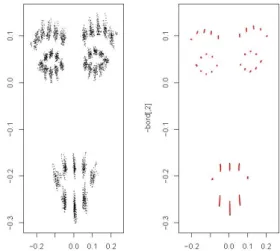
Consider a geometric object, as for example a flat fish or a skull. The "shape" of the object is defined as the class of equivalence obtained under similarity transformations, which are translations, rotations and scaling [12]. The main aims in order to study shapes are to reconstruct their evolution in time and to classify them. For example we can be interested in the shape of a particular species along its growth or to classify the shapes in different groups. Data from a shape are often realized as a set of points, as you can see on the left side of figure 1. In medical imaging, shadows and noise make the contour of the object not clear. Usually, experts identify a finite number of points, called landmarks. The landmark coordinates depend on the registration of the object in a coordinate system. [5, 13]. A realistic drawing of a cross-sectional rat cranium with eight landmarks is represented in figure 2.
Suppose to have a population of n planar objects Sj, j = 1, . . . , n, consisting of a fixed number K of landmarks labeled on some common coordinate system. Denote the landmarks Euclidean coordinates of the j-th object Sj with µj = (µj1, µj2, ..., µjK) where
µjk = (µjk1, µjk2), k = 1, . . . , K. The mean shape
is defined as ¯µ = 1nPn
j=1µj. For the k-landmark,
an estimate of the coordinates covariance matrix Σk is given by Σk= 1 n n X j=1 (µjk− ¯µk)(µjk− ¯µk)T
where ¯µk denotes the k-th landmark coordinates
FIG. 1. (color online) On the left side, Real data; on the right side, Geodesics from the model.
FIG. 2. (color online) Realistic drawing of a cross section of a rat cranium with the eight landmarks used in the analysis.
of the mean shape. Let S be a given shape from the population:
S = {µ1, µ2, . . . , µK} (3)
with generic element µk = (µk1, µk2) for k =
1, . . . , K. Assuming a diagonal covariance matrix [2], the k-th landmark may be represented by a bivariate Gaussian density as follows:
f (x | θk= (µk, Σk)) = (2π)−1
×(det Σk)−12exp{−1
2(x − µk)
TΣ−1
with x being a generic 2-dimensional vector and Σk given by
Σk= diag(σk12 , σ2k2) (5)
where σ2k = (σ2k1, σk22 ) is the vector of the variances of µk.
In the previous representation, the means represent the geometric coordinates of the landmark, which capture uncertainties that arise in landmark placement due to measurement errors. The variances are hidden coordinates reflecting natural variability across the population of shapes. Equation (4) assigns to the k-th landmark both the coordinates θk = (µk, σk) on
the 4-dimensional manifold which is the product of two upper half planes. Then, Riemannian metrics may be defined on the Gaussian densities manifold, where we are modelling the shapes. The induced geodesics may be used to reconstruct the intermediate shapes from those at two different times and also to predict, for a short time, the evolution of the shape from its past. In [1], the geodesics are determined by the Fisher-Rao metric. They minimize the information in the Fisher sense and are obtained as product of two geodesics in the hyperbolic plane. As an application, the rat calvarial data set [4] was used. It corresponds to 8 landmarks digitized in two dimensions on the skull midsagittal section of 21 rats, which have been collected at ages of 7, 14, 21, 30, 40, 60, 90, 150 days. In figure 3, the geodesic paths (solid lines) are displayed from the mean shape at time t = 14 days (dash-dotted line) to the mean shape at time t = 21 days (dashed line).
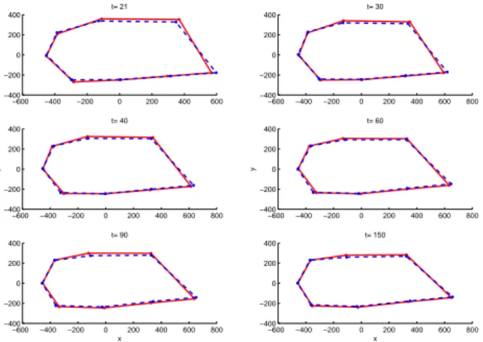
Besides, in figure 4, the observed (dashed lines) and estimated (solid lines) mean shapes from day 21 to day 150 are displayed.
The model works also starting from "non-geometrical" coordinates of an object, as we showed for Keratoconus which is a pathology affecting the corneal shape, producing serious problems to the vision. Corneal tomography gives numerical data of the axial and tangential algorithms which we can use as coordinates of cornea points. Therefore we proposed to apply our model in order to reconstruct the intermediate steps from an initial situation to the outbreak of the disease. −600 −400 −200 0 200 400 600 800 −300 −200 −100 0 100 200 300 400 x y 7 3 2 1 8 5 4 6
FIG. 3. (color online) Mean shape at time t = 14 days (dash-dotted line); mean shape at time t = 21 days (dashed line); geodesic paths (solid lines) from t = 14 to t = 21. −600 −400 −200 0 200 400 600 −400 −200 0 200 400 t= 21 −600 −400 −200 0 200 400 600 800 −400 −200 0 200 400 t= 30 −600 −400 −200 0 200 400 600 800 −400 −200 0 200 400 t= 40 y −600 −400 −200 0 200 400 600 800 −400 −200 0 200 400 t= 60 y −600 −400 −200 0 200 400 600 800 −400 −200 0 200 400 t= 90 x −600 −400 −200 0 200 400 600 800 −400 −200 0 200 400 t= 150 x
FIG. 4. (color online) Rat data set: observed (dashed lines) and estimated (solid lines) mean shapes from time t = 21 to day t = 150 days.
The geodesic distances can be used for cluster analysis of shapes, as it will be shown in the following section.
4. Clustering of shapes
In classical Shape Analysis, Procrustes methods [14] are used to compare shapes of different objects. Precisely on some common coordinates system, two objects are scaled, rotated and translated so that their landmarks
0 1 2 3 4 5 6 0 1 2 3 4 5 6 unregistered -3 -2 -1 0 1 2 3 -1.5 -1 -0.5 0 0.5 1 1.5 registered
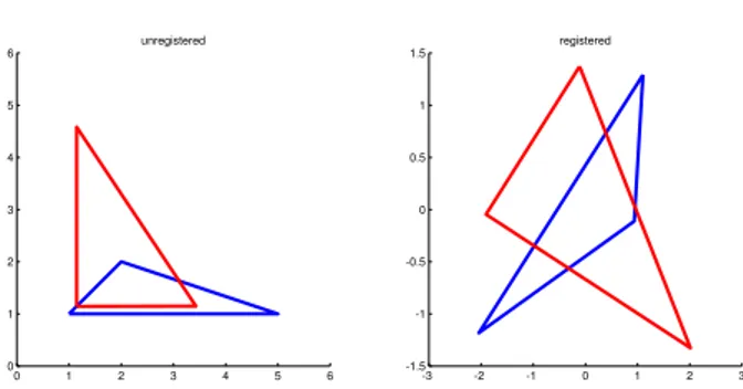
FIG. 5. (color online)The left panel shows original configurations of two triangle classes, while the right panel shows the two shapes registered with Ordinary Procrustes Analysis
lie as close as possible to each other with respect to the Euclidean distance. In other words, the minimization problem regarding the sum of the Euclidean distances of the corresponding landmarks of the two objects has to be solved. Such minimum is called the Procrustes distance of the two shapes. For example, the left panel of figure (5) shows the original configurations of triangles while in the right panel there are the two triangles obtained using ordinary Procrustes Analysis. Let S and S0 two planar shapes registered on a common coordinate system and parameterized as follows: S = (θ1, . . . , θK) and
S0= (θ01, . . . , θ0K). The geodesic distances between landmarks allow to define a distance of the two shapes S and S0. Precisely a shape metric, for measuring the difference between S and S0, can be obtained by taking the sum of the geodesic distances between the corresponding landmarks of the two shapes, according to the following definition: D(S, S0) = K X k=1 d(θk, θk0). (6)
Then a clustering of shapes, using in turn, as distance d, the distance dF induced from Fisher-Rao metric and the Wasserstein distance dW, can be done following the standard methodology. In [2], the proposed methodology has been applied for clustering shapes of a series of specimens belonging to three different flatfishes species. For
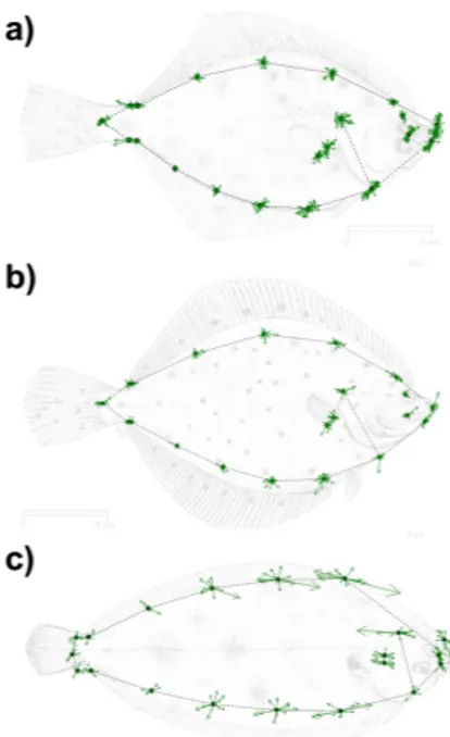
the experiment, the scheme of 21 landmarks was digitized for each individual of the three species, as in figure 6.
FIG. 6. (color online) Landmark configuration collected on (a) Platichthys flesus, (b) Pleuronectes platessa, and (c) Solea solea. 1, snout tip; 2, 3 and 4, points of maximum curvature of the peduncle; 5, insertion of the operculum on the lateral profile; 6, posterior extremity of premaxillar; 7 and 8, centers of the eyes; 9, beginning of the lateral line; 10 and 11, superior and inferior insertion of the pectoral fin; 12-16, semi- landmarks collected on dorsal fin; 17-20, semi-landmarks collected on anal fin; 21, insertion of first ray of the pelvic fin.
Pairwise distances of all shapes were computed with respect to different metrics: Procrustes distance dP and Fisher-Rao geodesic distances using isotropic covariance matrix, dR,
and diagonal covariance matrix, dF. The isotropic
case requires the choice of the free parameter σ2. In order to test the sensitiveness of the final clustering with respect to changes in the value of σ2, three different values of σ2 were considered
and given by the first (dR1), the second (dR2) and
the third quartile (dR3) of the variances of the
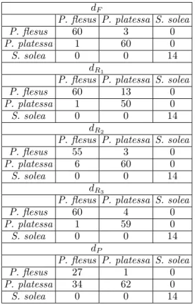
landmarks. The obtained distance matrices were then used in a hierarchical clustering algorithm and results, for each distance considered in the paper, are reported in terms of confusion matrices (Table 1). The results show that the specimens of S. solea, which represent the out-group, were
correctly identified by the clustering procedure independently of the selected distance measure. In contrast, a variable number of miss-classified specimens of P. flesus and P. platessa was always present. Some specimens of P. flesus were preferentially classified as P. platessa when the Fisher-Rao distance with σ2 given by the second quartile (dR2) was used, while the opposite miss classification (specimens of P. platessa classified as P. flesus) was more rare.
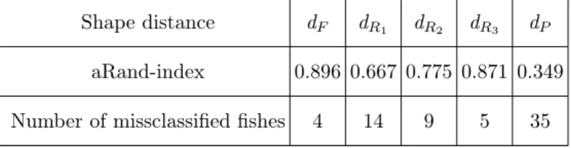
The behaviour of the clustering has been further evaluated by the aRand index [15] and classification error. Results for the solutions with three clusters are reported in Table 2 and show that the shape metric with the varying variance representation leads to the best performance in recovering the true cluster structure. Only 4 fishes were miss-classified with the Fisher-Rao distance dF which takes into account the variances of
the landmarks coordinates. Indeed, figure 7 gives evidence of some differences in the landmarks variability both along the horizontal axis and the vertical axis. For example, a larger variability is observed at landmarks n. 9, 13, 14, 15, 18, 19 and 20 of the S. solea species. The distance dR
assumes an isotropic covariance matrix and could be regarded as a fixed variance model. It does not consider these differences since it assumes the same variability for each landmark both in the horizontal and the vertical directions. This distance results in a worse cluster recovery with different behaviours depending on the value of the free parameter σ2. In particular, as the value of the free parameter σ2 increases, the ability to recognize the true cluster structure increases. For this particular data set, the Procrustes distance turns out to have a very poor performance in terms of cluster recovery.
5. K-means clustering algorithm In [3] the shape distances derived from Fisher-Rao metric and Wasserstein distance are implemented in two different generalized K-means algorithms, Type 1 and Type 2. While in the Type
FIG. 7. (color online) The full Procrustes mean shapes: (a) Platichthys flesus, (b) Pleuronectes platessa, and (c) S. solea. Vectors drawn from the mean to the full Procrustes coordinate of each landmark.
1 algorithm the landmark coordinates variances are assumed isotropic across the clusters, in Type 2 the variances are allowed to vary among the clusters. The task is clustering a set of n shapes, S1, S2, . . . , Sninto G different clusters, denoted as
C1, C2, . . . , CG.
5.1. Type 1 algorithm
1 Initial step:
Compute the variability of the k-th landmark coordinates σk2 = (σk12 , σk22 ), for k = 1, . . . , K.
Randomly assign the n shapes,
S1, S2, . . . , Sn into G clusters,
C1, C2, . . . , CG.
For g = 1, . . . , G calculate the cluster center cg = (θg1, . . . , θ
g
component θgk = (µgk, σk2) obtained as
θkg = ng1 P
i∈Cgθik, where ng is the number
of elements in the cluster Cg and θik
is the k-th coordinate of Si given by
θki = (µik, σ2k).
2 Classification:
For each shape Si, compute the distances
to the G cluster centers c1, c2, . . . , cG.
The generic distance between the shape Si and the cluster center cg is given by:
D(Si, cg) = K
X
k=1
d(θik, θkg).
Assign Si to cluster h that minimizes the
Table 1. Confusion matrices returned by the clustering algorithm based on the different distances. The outputs of the clustering procedure are in rows, the reference in columns.
dF
P. flesus P. platessa S. solea
P. flesus 60 3 0
P. platessa 1 60 0
S. solea 0 0 14
dR1
P. flesus P. platessa S. solea
P. flesus 60 13 0
P. platessa 1 50 0
S. solea 0 0 14
dR2
P. flesus P. platessa S. solea
P. flesus 55 3 0
P. platessa 6 60 0
S. solea 0 0 14
dR3
P. flesus P. platessa S. solea
P. flesus 60 4 0
P. platessa 1 59 0
S. solea 0 0 14
dP
P. flesus P. platessa S. solea
P. flesus 27 1 0 P. platessa 34 62 0 S. solea 0 0 14 distance: D(Si, ch) = min g D(Si, cg). 3 Renewal step:
Compute the new cluster centers of the renewed clusters c1, . . . , cG.
The k-th component of the g-th cluster center cg is defined as θkg = ng1 P
i∈Cgθki.
4 Repeat 2 and 3 until convergence.
5.2. Type 2 algorithm
1 Initial step:
Randomly assign the n shapes,
S1, S2, . . . , Sn into G clusters,
C1, C2, . . . , CG.
In each cluster compute the variability of the k-th landmark coordinates σgk2 = (σgk12 , σgk22 ), for k = 1, . . . , K and g = 1, . . . , G.
Calculate the cluster center cg =
(θ1g, . . . , θgK) with k-th component θkg = (µgk, σgk2 ) obtained as θ g k = ng1 P i∈Cgθki
for g = 1, . . . , G, where ng is the
number of elements in the cluster Cg
and θik= (µik, σgk2 ) for i ∈ Cg.
2 Classification:
For each shape Si, compute the distances
to the G cluster centers c1, c2, . . . , cG.
The generic distance between the shape Si and the cluster center cg is given by:
D(Si, cg) = K
X
k=1
d(θki, θgk).
Assign Si to cluster h that minimizes the distance:
D(Si, ch) = min
Table 2: a-Rand index and number of miss-classified fishes. Shape distance dF dR1 dR2 dR3 dP
aRand-index 0.896 0.667 0.775 0.871 0.349 Number of missclassified fishes 4 14 9 5 35
3 Renewal step:
Update the variability of the k-th landmark coordinates in each cluster by computing σ2gk = (σ2gk1, σgk22 ), for k = 1, . . . , K and for g = 1, . . . , G.
Calculate the new cluster centers of the renewed clusters c1, . . . , cG.
The k-th component of the g-th cluster center cg is defined as θgk= ng1 Pi∈Cgθik.
4 Repeat 2 and 3 until convergence.
6. Conclusions
In this paper, Information Geometry tools are used to study complex shapes described
by a finite number of landmarks. In particular shape distances derived from the Fisher-Rao and Wasserstein metrics are defined. The aim is to cluster shapes and compare the discriminative power of such distances with respect to a K-means algorithms. More general shape measures, for example induced by α-divergences, will be object of a future work.
References
[1] A. De Sanctis and S. A. Gattone, European Physical Journal, Special Topics 225, 1271 (2016).
[2] S. A. Gattone, A. De Sanctis, T. Russo, and D. Pulcini, Phisica A Statistical Mechanics and its Applications 487, 93 (2017).
[3] S. A. Gattone, A. De Sanctis, S. Puechmorel, and F. Nicol, Entropy 20 (9), 647 (2018).
[4] F. L. Bookstein, Morphometric Tools for Landmark Data: Geometry and Biology (Cambridge University Press, 1991).
[5] D. Kendall, Bulletin of the London Mathematical Society 16, 81 (1984).
[6] T. Cootes, C. Taylor, D. Cooper, and J. Graham, Computer Vision and Image Understanding 61, 38 (1995).
[7] C. J. Brignell, I. L. Dryden, S. A. Gattone, B. Park, S. Leask, W. J. Browne, and S. Flynn,
Biostatistics 11(4), 609 (2010).
[8] S. Amari and H. Nagaoka, Translations of mathematical monographs 191, AMS & Oxford University Press, Providence (2000).
[9] M. K. Murray and J. W. Rice, Differential Geometry and Statistics (Chapman & Hall, 1984).
[10] S. Costa, S. Santos, and J. Strapasson, Discrete Applied Mathematics 197, 59 (2015).
[11] A. Takatsu, Osaka Journal of Mathematics 48, 1005 (2011).
[12] I. L. Dryden and K. V. Mardia, Statistical Shape Analysis (John Wiley & Sons, London, 1998). [13] F. Bookstein, Statistical Science 1, 181 (1986). [14] C. R. Goodall, Journal of the Royal Statistical
Society, Series B 53, 285 (1991).
[15] L. Hubert and P. Arabie, Journal of Classification 2, 193 (1985).