© Author(s) 2017. This work is distributed under the Creative Commons Attribution 3.0 License.
Integrating faults and past earthquakes into a probabilistic
seismic hazard model for peninsular Italy
Alessandro Valentini1, Francesco Visini2, and Bruno Pace1
1DiSPUTer, Università degli Studi “Gabriele d’Annunzio” Chieti-Pescara, Chieti, Italy 2Istituto Nazionale di Geofisica e Vulcanologia, L’Aquila, Italy
Correspondence to: Alessandro Valentini ([email protected]) Received: 27 January 2017 – Discussion started: 6 February 2017
Revised: 6 October 2017 – Accepted: 17 October 2017 – Published: 22 November 2017
Abstract. Italy is one of the most seismically active countries in Europe. Moderate to strong earthquakes, with magnitudes of up to ⇠ 7, have been historically recorded for many active faults. Currently, probabilistic seismic hazard assessments in Italy are mainly based on area source models, in which seis-micity is modelled using a number of seismotectonic zones and the occurrence of earthquakes is assumed uniform. How-ever, in the past decade, efforts have increasingly been di-rected towards using fault sources in seismic hazard models to obtain more detailed and potentially more realistic patterns of ground motion. In our model, we used two categories of earthquake sources. The first involves active faults, and us-ing geological slip rates to quantify the seismic activity rate. We produced an inventory of all fault sources with details of their geometric, kinematic, and energetic properties. The associated parameters were used to compute the total seis-mic moment rate of each fault. We evaluated the magnitude– frequency distribution (MFD) of each fault source using two models: a characteristic Gaussian model centred at the max-imum magnitude and a truncated Gutenberg–Richter model. The second earthquake source category involves grid-point seismicity, with a fixed-radius smoothed approach and a his-torical catalogue were used to evaluate seismic activity. Un-der the assumption that deformation is concentrated along faults, we combined the MFD derived from the geometry and slip rates of active faults with the MFD from the spatially smoothed earthquake sources and assumed that the smoothed seismic activity in the vicinity of an active fault gradually de-creases by a fault-size-driven factor. Additionally, we com-puted horizontal peak ground acceleration (PGA) maps for return periods of 475 and 2475 years. Although the ranges and gross spatial distributions of the expected accelerations
obtained here are comparable to those obtained through methods involving seismic catalogues and classical zonation models, the spatial pattern of the hazard maps obtained with our model is far more detailed. Our model is characterized by areas that are more hazardous and that correspond to mapped active faults, while previous models yield expected acceler-ations that are almost uniformly distributed across large re-gions. In addition, we conducted sensitivity tests to deter-mine the impact on the hazard results of the earthquake rates derived from two MFD models for faults and to determine the relative contributions of faults versus distributed seismic activity. We believe that our model represents advancements in terms of the input data (quantity and quality) and method-ology used in the field of fault-based regional seismic hazard modelling in Italy.
1 Introduction
In this paper, we present the results of an alternative seismo-genic source model for use in a probabilistic seismic hazard assessment (PSHA) for Italy that integrates active fault and seismological data. The use of active faults as an input for seismic hazard analysis is a consolidated approach in many countries characterized by high strain rates and seismic re-leases, as shown, for example, by Field et al. (2015) in Cali-fornia and Stirling et al. (2012) in New Zealand. Moreover, in recent years, active fault data have also been successfully in-tegrated into seismic hazard studies or models in regions with moderate-to-low strain rates, such as SE Spain (e.g. Garcia-Mayordomo et al., 2007), France (e.g. Scotti et al., 2014), and central Italy (e.g. Peruzza et al., 2011).
In Europe, a working group of the European Seismolog-ical Commission, named Fault2SHA, is discussing fault-based seismic hazard modelling (https://sites.google.com/ site/linkingfaultpsha/home). The working group, created to encourage exchange among field geologists, fault modellers, and seismic hazard practitioners, and it is a community initia-tive with long-term vision on studying the acinitia-tive faults. The work we are presenting here stems from the activities of the Fault2SHA working group.
Combining active faults and background sources is one of the key aspects in this type of approach. Although the methodology remains far from identifying a standard proce-dure, common approaches combine active faults and back-ground sources by applying a threshold magnitude, generally between 5.5 and 7, above which seismicity is modelled as oc-curring on faults and below which seismicity is modelled via a smoothed approach (e.g. Akinci et al., 2009; Danciu et al., 2017), area sources (e.g. the so-called FSBG model in the 2013 European Seismic Hazard Model, ESHM13; Woessner et al., 2015), or a combination of the two (Field et al., 2015; Pace et al., 2006).
Another important aspect in the use of active faults to build a seismogenic source model is the use of an appropri-ate magnitude–frequency distribution (MFD) to characterize the temporal model describing the seismic activity of faults. Gutenberg–Richter (GR) and characteristic earthquake mod-els are commonly used, and the choice sometimes depends on the knowledge of the fault and data availability. Often, the choice of the “appropriate” MFD for each fault source is a difficult task because palaeoseismological studies are scarce, and it is often difficult to establish clear relationships between mapped faults and historical seismicity. Recently, Field et al. (2017) discussed the effects and complexity of the choice, highlighting how often the GR model results are not consistent with data; however, in other cases, uncharac-teristic behaviour, with rates smaller than the maximum, are possible. The discussion is open (see for example the dis-cussion by Kagan et al., 2012) and far from being solved with the available observations, including both seismological and/or geological/palaeoseismological observations. In this work, we explore the calculations of these two MFDs, a char-acteristic Gaussian model and a truncated Gutenberg–Richter model, to explore the epistemic uncertainties and to consider a mixed model as a so-called “expert judgment” model. This mixed model approach, in which we assigned one of the two MFDs to each fault source, is useful for comparison analysis. The rationale of the choice of the MFD of each fault source is explained in detail later in this paper. However, this approach obviously does not solve this issue, which can be treated as epistemic uncertainties using logic tree or random sampling, but in any case, the choice of MFD remains an open question in fault-based PSHA.
In Italy, the current national PSH model for building code (Stucchi et al., 2011) is based on area sources and the clas-sical Cornell approach (Cornell, 1968), in which the
oc-currence of earthquakes is assumed uniform in the defined seismotectonic zones. However, we believe that more effort must be directed towards using geological data (e.g. fault sources and palaeoseismological information) in PSHA to use slip rates that describe longer seismic cycles to match the larger magnitudes, extending the observational time re-quired to capture the recurrence of large-magnitude events and therefore improve the reliability of seismic hazard as-sessments. In fact, as highlighted by the 2016–2017 seis-mic sequences in central Italy, a zone-based source model is not able to model local spatial variations in ground mo-tion (Meletti et al., 2016), whereas a fault-based model can provide insights for aftershock time-dependent hazard anal-ysis (Peruzza et al., 2016). In conclusion, even if the main purpose of this work is to integrate active faults into hazard calculations for the Italian territory, this study does not rep-resent an official update of the seismic hazard model of Italy.
2 Source inputs
Two earthquake-source inputs are considered in this work. The first is a fault source input that is based on active faults and uses the geometries and slip rates of known active faults to compute activity rates over a certain range of magnitudes. The second is a classical smoothed approach that accounts for the rates of expected earthquakes with a minimum mo-ment magnitude (Mw) of 4.5 but excludes earthquakes
asso-ciated with known faults based on a modified earthquake cat-alogue. Note that our seismogenic source requires the com-bination of the two source inputs related to the locations of expected seismicity rates into a single source model. There-fore, these two earthquake-source inputs are not independent but complementary, in both the magnitude and frequency tribution, and together account for spatial and temporal dis-tribution of the seismicity in Italy.
In the following subsections, we describe the two source inputs and how they are combined in the seismogenic source model.
2.1 Fault source input
In seismic hazard assessment, an active fault is a struc-ture that exhibits evidence of activity in the late Quater-nary, has a demonstrable or potential capability of gener-ating major earthquakes, and is capable of future reactiva-tion (e.g. Machette, 2000; Danciu et al., 2017). The evi-dence of Quaternary activity can be geomorphological and/or palaeoseismological when activation information from in-strumental seismic sequences and/or association with histor-ical earthquakes is not available. Fault source data and loca-tion are useful for seismic hazard studies, and we compiled a database for Italy via the analysis and synthesis of neotec-tonic and seismotecneotec-tonic data from approximately 90 pub-lished studies of 110 faults across Italy. Our database
in-cluded, but was not limited to, the Database of Individual Seismogenic Sources (DISS vers. 3.2.0, http://diss.rm.ingv. it/diss/), which is already available for Italy. It is impor-tant to highlight that the DISS is currently composed of two main categories of seismogenic sources: individual and com-posite sources. The latter are defined by the DISS’ authors as a “simplified and three-dimensional representation of a crustal fault containing an unspecified number of seismo-genic sources that cannot be singled out. Composite seis-mogenic sources are not associated with a specific set of earthquakes or earthquake distribution”, and therefore are not useful for our PSHA approach; the former is “a sim-plified and three-dimensional representation of a rectangu-lar fault plane. Individual seismogenic sources are assumed to exhibit characteristic behaviour with respect to rupture length/width and expected magnitude” (http://diss.rm.ingv.it/ diss/index.php/about/13-introduction). Even if in agreement with our approach, we note that some of the individual seis-mogenic sources in the DISS are based on geological and palaeoseismological information, and many others used the Boxer code (Gasperini et al., 1999) to calculate the epicentre, moment magnitude, size, and orientation of a seismic source from observed macroseismic intensities. We carefully anal-ysed the individual sources and some related issues: (i) the lack of updates to the geological information of some indi-vidual sources and (ii) the nonconformity between the input data used by DISS in Boxer and the latest historical seismic-ity (CPTI15) and macroseismic intensseismic-ity (DBMI15) publica-tions. Thus, we performed a full review of the fault database. We then compiled a fault source database as a synthesis of works published over the past 20 years, including DISS, us-ing all updated and available geological, palaeoseismologi-cal, and seismological data (see Supplement for a complete list of references). We consider our database as complete as possible in terms of individual seismogenic sources, and it contains all the parameters necessary to construct an input data set for fault-based PSHA.
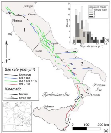
The resulting database of normal and strike-slip active and seismogenic faults in peninsular Italy (Fig. 1, Tables 1 and 2; see Supplement) includes all the available geometric, kine-matic, slip rate, and earthquake source-related information. In the case of missing data regarding the geometric param-eters of dip and rake, we assumed typical dip and rake val-ues of 60 and 90 respectively for normal faults and 90 and 0 or 180 respectively for strike-slip faults. In this paper, only normal and strike-slip faults are used as fault source in-puts. We decided not to include thrust faults in the present study because, with the methodology proposed in this study (as discussed later in the text), the maximum size of a single-rupture segment must be defined, and segmentation criteria have not been established for large thrust zones. Moreover, our method uses long-term geological slip rates to derive ac-tive seismicity rates, and sufficient knowledge of these values is not available for thrust faults in Italy. Because some areas of Italy, such as the NE sector of the Alps, Po Valley, the
Figure 1. (a) Map of normal and strike-slip active faults used in this study. The colour scale indicates the slip rate.(b) Histogram of the slip rate distribution in the entire study area and in three sub-sectors. The numbers 1, 2, and 3 represent the northern Apennines, central–southern Apennines, and Calabrian–Sicilian coast regions respectively. The dotted black lines are the boundaries of the re-gions.
offshore sector of the central Adriatic Sea, and SW Sicily, may be excluded by this limitation, we are considering an update to our approach to include thrust faults and volcanic sources in a future study. The upper and lower boundaries of the seismogenic layer are mainly derived from the analysis of Stucchi et al. (2011) of the Italian national seismic hazard model and locally refined by more detailed studies (Boncio et al., 2011; Peruzza et al., 2011; Ferranti et al., 2014).
Based on the compiled database, we explored three main aspects associated with defining a fault source input: the slip rate evaluation, the segmentation model and the expected seismicity rate calculation.
2.1.1 Slip rates
Slip rates control fault-based seismic hazards (Main, 1996; Roberts et al., 2004; Bull et al., 2006; Visini and Pace, 2014) and reflect the velocities of the mechanisms that operate dur-ing continental deformation (e.g. Cowie et al., 2005). More-over, long-term observations of faults in various tectonic contexts have shown that slip rates vary in space and time (e.g. Bull et al., 2006; Nicol et al., 2006, 2010; McClymont
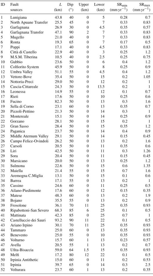
Table 1. Geometric parameters of the fault sources. L, along-strike length; dip, inclination angle of the fault plane; upper and lower, the thickness bounds of the local seismogenic layer; SRminand SRmax, the minimum and maximum slip rates assigned to the sources using the
references available (see Supplement); and ID, the fault number identifier.
ID Fault L Dip Upper Lower SRmin SRmax sources (km) ( ) (km) (km) (mm yr 1) (mm yr 1) 1 Lunigiana 43.8 40 0 5 0.28 0.7 2 North Apuane Transfer 25.5 45 0 7 0.33 0.83 3 Garfagnana 26.9 30 0 4.5 0.35 0.57 4 Garfagnana Transfer 47.1 90 2 7 0.33 0.83 5 Mugello 21.0 40 0 7 0.33 0.83 6 Ronta 19.3 65 0 7 0.17 0.5 7 Poppi 17.1 40 0 4.5 0.33 0.83 8 Città di Castello 22.9 40 0 3 0.25 1.2 9 M.S.M. Tiberina 10.5 40 0 2.5 0.25 0.75 10 Gubbio 23.6 50 0 6 0.4 1.2 11 Colfiorito System 45.9 50 0 8 0.25 0.9 12 Umbra Valley 51.1 55 0 4.5 0.4 1.2 13 Vettore-Bove 35.4 50 0 15 0.2 1.05 14 Nottoria-Preci 29.0 50 0 12 0.2 1 15 Cascia-Cittareale 24.3 50 0 13.5 0.2 1 16 Leonessa 14.9 55 0 12 0.1 0.7 17 Rieti 17.6 50 0 10 0.25 0.6 18 Fucino 82.3 50 0 13 0.3 1.6 19 Sella di Corno 23.1 60 0 13 0.35 0.7 20 Pizzoli-Pettino 21.3 50 0 14 0.3 1 21 Montereale 15.1 50 0 14 0.25 0.9 22 Gorzano 28.1 50 0 15 0.2 1 23 Gran Sasso 28.4 50 0 15 0.35 1.2 24 Paganica 23.7 50 0 14 0.4 0.9 25 Middle Aternum Valley 29.1 50 0 14 0.15 0.45 26 Campo Felice-Ovindoli 26.2 50 0 13 0.2 1.6 27 Carsoli 20.5 50 0 11 0.35 0.6 28 Liri 42.5 50 0 11 0.3 1.26 29 Sora 20.4 50 0 11 0.15 0.45 30 Marsicano 20.0 50 0 13 0.25 1.2 31 Sulmona 22.6 50 0 15 0.6 1.35 32 Maiella 21.4 55 0 15 0.7 1.6 33 Aremogna C.Miglia 13.1 50 0 15 0.1 0.6 34 Barrea 17.1 55 0 13 0.2 1 35 Cassino 24.6 60 0 11 0.25 0.5 36 Ailano-Piedimonte 17.6 60 0 12 0.15 0.35 37 Matese 48.3 60 0 13 0.2 1.9 38 Bojano 35.5 55 0 13 0.2 0.9 39 Frosolone 36.1 70 11 25 0.35 0.93 40 Ripabottoni-San Severo 68.3 85 6 25 0.1 0.5 41 Mattinata 42.3 85 0 25 0.7 1 42 Castelluccio dei Sauri 93.2 90 11 22 0.1 0.5 43 Ariano Irpino 30.1 70 11 25 0.35 0.93 44 Tammaro 25.0 60 0 13 0.35 0.93 45 Benevento 25.0 55 0 10 0.35 0.93 46 Volturno 15.7 60 1 13 0.23 0.57 47 Avella 20.5 55 1 13 0.2 0.7 48 Ufita-Bisaccia 59.0 64 1.5 15 0.35 0.93 49 Melfi 17.2 80 12 22 0.1 0.5 50 Irpinia Antithetic 15.0 60 0 11 0.2 0.53 51 Irpinia 39.7 65 0 14 0.3 2.5 52 Volturara 23.7 60 1 13 0.2 0.35
Table 1. Continued.
ID Fault L Dip Upper Lower SRmin SRmax sources (km) ( ) (km) (km) (mm yr 1) (mm yr 1) 53 Alburni 20.4 60 0 8 0.35 0.7 54 Caggiano–Diano Valley 46.0 60 0 12 0.35 1.15 55 Pergola-Maddalena 50.6 60 0 12 0.20 0.93 56 Agri 34.9 50 5 15 0.8 1.3 57 Potenza 17.8 90 15 21 0.1 0.5 58 Palagianello 73.3 90 13 22 0.1 0.5 59 Monte Alpi 10.9 60 0 13 0.35 0.9 60 Maratea 21.6 60 0 13 0.46 0.7 61 Mercure 25.8 60 0 13 0.2 0.6 62 Pollino 23.8 60 0 15 0.22 0.58 63 Castrovillari 10.3 60 0 15 0.2 1.15 64 Rossano 14.9 60 0 22 0.5 0.6 65 Crati West 49.7 45 0 15 0.84 1.4 66 Crati East 18.4 60 0 8 0.75 1.45 67 Lakes 43.6 60 0 22 0.75 1.45 68 Fuscalto 21.1 60 2 22 0.75 1.45 69 Piano Lago-Decollatura 25.0 60 1 15 0.23 0.57 70 Catanzaro North 29.5 80 3 20 0.75 1.45 71 Catanzaro South 21.3 80 3 20 0.75 1.45 72 Serre 31.6 60 0 15 0.7 1.15 73 Vibo 23.0 80 0 15 0.75 1.45 74 Sant’Eufemia Gulf 24.8 40 1 11 0.11 0.3 75 Capo Vaticano 13.7 60 0 8 0.75 1.45 76 Coccorino 13.3 70 3 11 0.75 1.45 77 Scilla 29.7 60 0 13 0.8 1.5 78 Sant’Eufemia 19.2 60 0 13 0.75 1.45 79 Cittanova-Armo 63.8 60 0 13 0.45 1.45 80 Reggio Calabria 27.2 60 0 13 0.7 2 81 Taormina 38.7 30 3 13 0.9 2.6 82 Acireale 39.4 60 0 15 1.15 2.3 83 Western Ionian 50.1 65 0 15 0.75 1.45 84 Eastern Ionian 39.3 65 0 15 0.75 1.45 85 Climiti 15.7 60 0 15 0.75 1.45 86 Avola 46.9 60 0 16 0.8 1.6
et al., 2009a, b; Gunderson et al., 2013; Benedetti et al., 2013; D’Amato et al., 2016), and numerical simulations (e.g. Robinson et al., 2009; Cowie et al., 2012; Visini and Pace, 2014) suggest that variability mainly occurs in response to interactions between adjacent faults. Therefore, understand-ing the temporal variability in fault slip rates is a key point in understanding the earthquake recurrence rates and their vari-ability.
To evaluate the minimum and maximum slip rates, which we assumed representative of the long-term slip rate variabil-ity over time, we used slip rates determined in different ways and at different timescales (e.g. at the decadal scale based on geodetic data or at longer scales based on the displace-ment of Holocene or Plio-Pleistocene horizons). These val-ues were derived from approximately 65 available neotecton-ics, palaeoseismology, and seismotectonics papers (see Sup-plement). In this work, we used the mean of the minimum
and maximum slip rate values listed in Table 1 and assumed that they are representative of the long-term behaviour (over the past 15 kyr in the Apennines). Because a direct compar-ison of slip rates over different time intervals obtained by different methods may be misleading (Nicol et al., 2009), we cannot exclude the possibility that uncertainties and er-rors compilation could affect the original data in some cases. The discussion of these possible biases and their evaluation via statistically derived approaches (e.g. Gardner et al., 1987; Finnegan et al., 2014; Gallen et al., 2015) is beyond the scope of this paper and will be explored in future work. Moreover, we are assuming that slip rate values used are representative of seismic movements, and aseismic factors are not taken into account. Therefore, we believe that investigating the effect of this assumption could be another issue explored in future work, for example, by differentiating between aseismic slip factors in different tectonic contexts.
Because 28 faults had no measured slip (or throw) rate (Fig. 1a), we proposed a statistically derived approach to as-sign a slip rate to these faults. Based on the slip rate spa-tial distribution shown in Fig. 1b, we subdivided the fault database into three large regions – the northern Apennines, central–southern Apennines, and Calabrian–Sicilian coast – and analysed the slip rate distribution in these three areas. Figure 1b indicates that the slip rates tend to increase from north to south. The fault slip rates in the northern Apennines range from 0.3 to 0.8 mm yr 1, with the most common values
ranging from approximately 0.5–0.6 mm yr 1; the slip rates
in the central–southern Apennines range from 0.3 to 1.0, and the most common rate is approximately 0.3 mm yr 1; the
slip rates in the southern area (Calabria and Sicily) range from 0.9 to 1.8, with the most common being approximately 0.9 mm yr 1.
Keeping in mind that average and minimum–maximum range of slip rate represents two different aspects of the slip rate behaviour of a fault (average long-term slip rate and its variability), we analysed them independently to assign values to active faults without measures.
The first step in assigning an average slip rate and a range of variability to the faults with unknown values is to identify the most representative distribution among known probabil-ity densprobabil-ity functions using the slip rate data from each of the three areas. We test five well-known probability density func-tions (Weibull, normal, exponential, inverse Gaussian, and gamma) against mean slip rate observations. The resulting function with the highest log-likelihood is the normal func-tion in all three areas. Thus, the mean value of the normal distribution is assigned to the faults with unknown values. We assign a value of 0.58 mm yr 1to faults in the northern
area, 0.64 mm yr 1to faults in the central–southern area, and
1.10 mm yr 1to faults in the Calabrian–Sicilian area. To
as-sign a range of slip rate variability to each of the three areas, we test the same probability density functions against slip rate variability observations. Similar to the mean slip rate, the probability density function with the highest log-likelihood is the normal function in all three areas. We assign a vari-ability of 0.25 mm yr 1 to the faults in the northern area,
0.29 mm yr 1to the faults in the central–southern area, and
0.35 mm yr 1to the faults in the Calabrian–Sicilian area.
2.1.2 Segmentation rules for delineating fault sources An important issue in the definition of fault source input is the formulation of segmentation rules. In fact, the question of whether structural segment boundaries along multi-segment active faults act as persistent barriers to a single rupture is critical to defining the maximum seismogenic potential of fault sources. In our case, the rationale behind the definition of a fault source is based on the assumption that the geomet-ric and kinematic features of a fault source are expressions of its seismogenic potential and that its dimensions are compat-ible for hosting major (Mw 5.5) earthquakes. Therefore, a
fault source may consist of a fault or an ensemble of faults that slip together during an individual major earthquake. A fault source is defined by a seismogenic master fault and its surface projection (Fig. 2a). Seismogenic master faults are separated from each other by first-order structural or geo-metrical complexities. Following the suggestions by Boncio et al. (2004) and Field et al. (2015), we imposed the fol-lowing segmentation rules in our case study: (i) 4 km fault gaps among aligned structures; (ii) intersections with cross structures (often transfer faults) extending 4 km along strike and oriented at nearly right angles to the intersecting faults; (iii) overlapping or underlapping en echelon arrangements with separations between faults of 4 km; (iv) bending 60 for more than 4 km; (v) average slip rate variability along a strike greater than or equal to 50 %; and (vi) changes in seis-mogenic thickness greater than 5 km among aligned struc-tures. Example applications of the above rules are illustrated in Fig. 2a.
By applying the above rules to our fault database, the 110 faults yielded 86 fault sources: 9 strike-slip sources and 77 normal-slip sources. The longest fault source is Castelluc-cio dei Sauri (fault number, ID in Table 1, 42, L = 93.2 km), and the shortest is Castrovillari (ID 63, L = 10.3 km). The mean length is 30 km. The dip angle varies from 30 to 90 , and 70 % of the fault sources have dip angles between 50 and 60 . The mean value of seismogenic thickness (ST) is approximately 12 km. The source with the largest ST is Mat-tinata (ID 41, ST = 25 km), and the source with the thinnest ST is Monte Santa Maria Tiberina (ID 9, ST = 2.5 km). This low value is due to the presence of an east-dipping low angle normal fault, the Alto-Tiberina Fault (Boncio et al., 2000), located a few kilometres west of the Monte Santa Maria Tiberina fault. Maximum observed moment magnitude val-ues (MObs) have been assigned to 35 fault sources (based on Table 2), and the values vary from 5.90 to 7.32. The fault source inputs are shown in Fig. 3.
2.1.3 Expected seismicity rates
Each fault source is characterized by data, such as kinematic, geometry, and slip rate information, which we use as inputs for the FiSH code (Pace et al., 2016) to calculate the global budget of the seismic moment rate allowed by the structure. This calculation is based on predefined size–magnitude re-lationships in terms of the maximum magnitude (Mmax) and
the associated mean recurrence time (Tmean). Table 1
sum-marizes the geometric parameters used as FiSH input pa-rameters for each fault source (seismogenic box) shown in Fig. 3. To evaluate Mmaxof each source, according to Pace
et al. (2016), we first computed and then combined up to five Mmax estimates (see example of the Paganica fault source in Fig. 2b, details in Pace et al., 2016). Specifically, these five Mmaxestimates are as follows: MMo based on the
cal-culated scalar seismic moment (Mo) and the application of the standard formula Mw= 2/3 (logMo 9.1); Hanks and
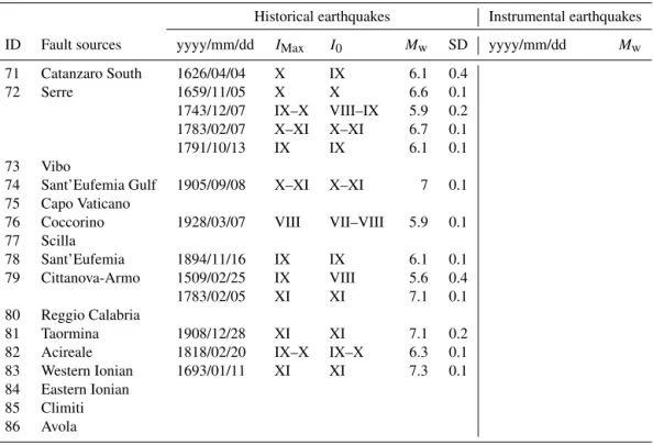
Table 2. Earthquake-source association adopted for fault sources. IMax, maximum intensity; I0, epicentral intensity; Mw, moment magnitude;
and SD, standard deviation of the moment magnitude. For references, see Supplement.
Historical earthquakes Instrumental earthquakes ID Fault sources yyyy/mm/dd IMax I0 Mw SD yyyy/mm/dd Mw 1 Lunigiana 1481/05/07 VIII VIII 5.6 0.4
1834/02/14 IX IX 6.0 0.1 2 North Apuane Transfer 1837/04/11 X IX 5.9 0.1 3 Garfagnana 1740/03/06 VIII VIII 5.6 0.2 1920/09/07 X X 6.5 0.1 4 Garfagnana Transfer 5 Mugello 1542/06/13 IX IX 6.0 0.2 1919/06/29 X X 6.4 0.1 6 Ronta 7 Poppi 8 Città di Castello 1269 IX IX 5.7 0.5 1389/10/18 VIII–IX VIII–IX 6 0.5 1458/04/26 IX IX 5.8 0.1 1789/09/30 5.9 9 M.S.M. Tiberina 1352/12/25 IX IX 6.3 0.2 1917/04/26 IX–X IX–X 6.0 0.1 10 Gubbio 1984/04/29 5.6 11 Colfiorito System 1279/04/30 X IX 6.2 0.2 1997/09/26 5.7 1747/04/17 IX IX 6.1 0.1 1997/09/26 6 1751/07/27 X X 6.4 0.1
12 Umbra Valley 1277 X VIII 5.6 0.5 1832/01/13 VIII X 6.4 0.1 1854/02/12 VIII 5.6 0.3 13 Vettore-Bove 2016/10/30 6.5 14 Nottoria-Preci 1328/12/01 X X 6.5 0.3 1979/09/19 5.8 1703/01/14 XI XI 6.9 0.1 1719/06/27 VIII VIII 5.6 0.3 1730/05/12 IX IX 6.0 0.1 1859/08/22 VIII–IX VIII–IX 5.7 0.3 1879/02/23 VIII VIII 5.6 0.3 15 Cascia-Cittareale 1599/11/06 IX IX 6.1 0.2 1916/11/16 VIII VIII 5.5 0.1 16 Leonessa 17 Rieti 1298/12/01 X IX–X 6.3 0.5 1785/10/09 VIII–IX VIII–IX 5.8 0.2 18 Fucino 1349/09/09 IX IX 6.3 0.1 1904/02/24 IX VIII–IX 5.7 0.1 1915/01/13 XI XI 7 0.1 19 Sella di Corno 20 Pizzoli-Pettino 1703/02/02 X X 6.7 0.1 21 Montereale 22 Gorzano 1639/10/07 X IX–X 6.2 0.2 1646/04/28 IX IX 5.9 0.4 23 Gran Sasso
24 Paganica 1315/12/03 VIII VIII 5.6 0.5 2009/06/04 6.3 1461/11/27 X X 6.5 0.5
25 Middle Aternum Valley 26 Campo Felice-Ovindoli 27 Carsoli 28 Liri 29 Sora 1654/07/24 X IX–X 6.3 0.2 30 Marsicano 31 Sulmona
Table 2. Continued.
Historical earthquakes Instrumental earthquakes ID Fault sources yyyy/mm/dd IMax I0 Mw SD yyyy/mm/dd Mw 32 Maiella 33 Aremogna C.Miglia 34 Barrea 1984/05/07 5.9 35 Cassino 36 Ailano-Piedimonte 37 Matese 1349/09/09 X–XI X 6.8 0.2 38 Bojano 1805/07/26 X X 6.7 0.1 39 Frosolone 1456/12/05 XI XI 7 0.1 40 Ripabottoni-San Severo 1627/07/30 X X 6.7 0.1 2002/10/31 5.7 1647/05/05 VII–VIII VII–VIII 5.7 0.4 1657/01/29 IX–X VIII–IX 6.0 0.2 41 Mattinata 1875/12/06 VIII VIII 5.9 0.1 1889/12/08 VII VII 5.5 0.1 1948/08/18 VII–VIII VII–VIII 5.6 0.1 42 Castelluccio dei Sauri 1361/07/17 X IX 6 0.5 1560/05/11 VIII VIII 5.7 0.5 1731/03/20 IX IX 6.3 0.1 43 Ariano Irpino 1456/12/05 IX IX 6.9 0.1 1962/08/21 6.2 0.1 44 Tammaro 1688/06/05 XI XI 7 0.1 45 Benevento 46 Volturno
47 Avella 1499/12/05 VIII VIII 5.6 0.5 48 Ufita-Bisaccia 1732/11/29 X–XI X–XI 6.8 0.1 1930/07/23 X X 6.7 0.1 49 Melfi 1851/08/14 X X 6.5 0.1 50 Irpinia Antithetic
51 Irpinia 1466/01/15 VIII–IX VIII–IX 6.0 0.2 1980/11/23 6.8 1692/03/04 VIII VIII 5.9 0.4
1694/09/08 X X 6.7 0.1 1853/04/09 IX VIII 5.6 0.2 52 Volturara
53 Alburni
54 Caggiano–Diano Valley 1561/07/31 IX–X X 6.3 0.1 55 Pergola-Maddalena 1857/12/16 6.5
1857/12/16 6.3 56 Agri
57 Potenza 1273/12/18 VIII–IX VIII–IX 5.8 0.5 1990/05/05 5.8 58 Palagianello
59 Monte Alpi 60 Maratea
61 Mercure 1708/01/26 VIII–IX VIII 5.6 0.6 1998/09/09 5.5 62 Pollino 63 Castrovillari 64 Rossano 1836/04/25 X IX 6.2 0.2 65 Crati West 1184/05/24 IX IX 6.8 0.3 1870/10/04 X IX–X 6.2 0.1 1886/03/06 VII–VIII VII–VIII 5.6 0.3 66 Crati East 1767/07/14 VIII–IX VIII–IX 5.9 0.2 1835/10/12 X IX 5.9 0.3 67 Lakes 1638/06/08 X X 6.8 0.1 68 Fuscalto 1832/03/08 X X 6.6 0.1 69 Piano Lago-Decollatura
Table 2. Continued.
Historical earthquakes Instrumental earthquakes ID Fault sources yyyy/mm/dd IMax I0 Mw SD yyyy/mm/dd Mw 71 Catanzaro South 1626/04/04 X IX 6.1 0.4 72 Serre 1659/11/05 X X 6.6 0.1 1743/12/07 IX–X VIII–IX 5.9 0.2 1783/02/07 X–XI X–XI 6.7 0.1 1791/10/13 IX IX 6.1 0.1 73 Vibo
74 Sant’Eufemia Gulf 1905/09/08 X–XI X–XI 7 0.1 75 Capo Vaticano
76 Coccorino 1928/03/07 VIII VII–VIII 5.9 0.1 77 Scilla 78 Sant’Eufemia 1894/11/16 IX IX 6.1 0.1 79 Cittanova-Armo 1509/02/25 IX VIII 5.6 0.4 1783/02/05 XI XI 7.1 0.1 80 Reggio Calabria 81 Taormina 1908/12/28 XI XI 7.1 0.2 82 Acireale 1818/02/20 IX–X IX–X 6.3 0.1 83 Western Ionian 1693/01/11 XI XI 7.3 0.1 84 Eastern Ionian
85 Climiti 86 Avola
Kanamori, 1979; IASPEI, 2005); two magnitude estimates using the Wells and Coppersmith (1994) empirical relation-ships for the maximum subsurface rupture length (MRLD) and maximum rupture area (MRA); an estimate that corre-sponds to the MObs, if available; and an estimate (MASP, ASP for aspect ratio) computed by reducing the fault length input if the aspect ratio (W / L) is smaller than the value eval-uated by the relation between the aspect ratio and rupture length of observed earthquake ruptures, as derived by Pe-ruzza and Pace (2002; not in the case of Paganica in Fig. 2b). In some cases, the use of MObs was useful to better constrain the seismogenic potential of individual seismogenic sources. For this reason and to take into account MObs in the estima-tion of Mmax, for each source we (i) calculated the maximum
expected magnitude (Mmax1) and the relative uncertainties
using only the scaling relationships and (ii) compared the maximum of observed magnitudes of the earthquakes poten-tially associated with the fault. If MObs was within the range of Mmax± 1 standard deviation, we considered the value and
recalculated a new Mmax(Mmax2) with a new uncertainty. If
MObs was larger than Mmax1+ 1 standard deviation, we
re-viewed the fault geometry and/or the earthquake-source as-sociation. Conversely, if MObs was lower then Mmax1 1
standard deviation we considered a GR behaviour for that source, without using the MObs in the Mmax2calculation. As
an example, for the Irpinia Fault (ID 51 in Tables 1 and 2), the characteristics of the 1980 earthquake (Mw⇠ 6.9) can be
used to evaluate Mmaxvia comparison with the Mmaxderived
from scaling relationships.
Because all the empirical relationships, as well as ob-served historical and recent magnitudes of earthquakes, are affected by uncertainties, the MomentBalance (MB) func-tion of the FiSH code (Pace et al., 2016) was used to account for these uncertainties. MB computes a probability density function (PDF) for each magnitude derived from empirical relationships or observations and summarizes the results as a maximum magnitude value with a standard deviation. The uncertainties in the empirical scaling relationship, in FiSH, are taken from the studies of Wells and Coppersmith (1994), Peruzza and Pace (2002), and Leonard (2010). Currently, the uncertainty in magnitude associated with the seismic mo-ment is fixed and set to 0.3, whereas the catalogue defines the uncertainty in MObs. Moreover, to combine the evaluated maximum magnitudes, MB creates a probability curve for each magnitude by assuming a normal distribution (Fig. 2). We assumed a two-sided un-truncated normal distribution of magnitudes. MB subsequently sums the probability density curves and fits the summed curve to a normal distribution to obtain the mean of the maximum magnitude Mmax and its
standard deviation.
Thus, a unique Mmax with a standard deviation is
com-puted for each source, and this value represents the maxi-mum rupture that is allowed by the fault geometry and the rheological properties.
Finally, to obtain the mean recurrence time of Mmax(i.e.
Tmean), we use the criterion of “segment seismic moment conservation” proposed by Field et al. (1999). This criterion divides the seismic moment that corresponds to Mmaxby the
Figure 2. (a) Conceptual model of active faults and segmentation rules adopted to define a fault source and its planar projection, forming a seismogenic box (modified from Boncio et al., 2004).(b) Example of FiSH code output (see Pace et al., 2016, for details) for the Paganica fault source showing the magnitude estimates from empirical relationships and observations, both of which are affected by uncertainties. In this example, four magnitudes are estimated: MMo (blue line), based on the calculated scalar seismic moment (Mo), is from the standard formula (IASPEI, 2005); MRLD (red line) and MRA (cyan line) correspond to estimates based on the maximum subsurface fault length and maximum rupture area from the empirical relationships of Wells and Coppersmith (1994) for length and area respectively; and MObs (magenta line) is the largest observed moment magnitude. The black dashed line represents the summed probability density curve (SumD), the vertical black line represents the central value of the Gaussian fit of the summed probability density curve (Mmax), and the horizontal
black dashed line represents its standard deviation ( Mmax). The input values that were used to obtain this output are provided in Table 1.
(c) Comparison of the magnitude–frequency distributions of the Paganica source, which were obtained using the CHG model (red line) and the TGR model (black line).
moment rate for given a slip rate:
Tmean=Char_Rate =1 10
(1.5Mmax+9.1)
µVLW , (1)
where Tmeanis the mean recurrence time in years, Char_Rate
is the annual mean rate of occurrence, Mmaxis the computed
mean maximum magnitude, µ is the shear modulus, V is the average long-term slip rate, and L and W are along-strike rupture length and down-dip width respectively. Finally, we calculated the seismic moment rate corresponding to Mmax
and the MFDs of expected seismicity. For each fault source, we use two endmember MFD models: (i) a characteristic Gaussian (CHG) model, a symmetric Gaussian curve (ap-plied to the incremental MFD values) centred on the Mmax
value of each fault with a range of magnitudes equal to 1 , and (ii) a truncated Gutenberg–Richter (TGR; Ordaz and Reyes, 1999; Kagan, 2002) model, with Mmaxas the upper
threshold and Mw= 5.5 as the minimum threshold for all
sources. We consider a constant b value equal to 1.0 for all faults, as single-source events are insufficient for calculating the required statistics; this value corresponds to the mean b value determined from the CPTI15 catalogue. The a values were computed with the ActivityRate tool of the FiSH code. ActivityRate calculated activity rates at magnitudes given by
each MFD, balancing the total MFD expected seismic mo-ment rate with the seismic momo-ment rate that was obtained based on Mmaxand Tmean(details in Field et al., 1999, 2015;
Pace et al., 2016; Woessner et al., 2015). In Fig. 2c, we show an example of the expected seismicity rates in terms of the annual cumulative rates for the Paganica source using the two above-described MFD models.
Finally, we create a so-called expert judgement model, called the mixed model, to determine the MFD for each fault source based on the earthquake-source associations. In this case, we decided that if an earthquake assigned to a fault source (see Table 2 for earthquake-source associations) has a magnitude lower than the magnitude range in the curve of the CHG model distribution, the TGR model is applied to that fault source. Otherwise, the CHG model, which peaks at the calculated Mmax, is applied. We decided to not use a
logic tree for every fault to capture the model options be-cause one of the aims of this work is to compare the different MFD choices in terms of results and impact in the hazard curves. Of course, errors in this approach can originate from the misallocation of historical earthquakes, and we cannot exclude the possibility that potentially active faults respon-sible for historical earthquakes have not yet been mapped.
Figure 3. Maps showing the fault source inputs as seismogenic boxes (see Fig. 2a). The colour scale indicates the activity rate. Solid and dashed lines (corresponding to the uppermost edge of the fault) are used to highlight our choice between the two endmembers of the MFD model adopted in the so-called mixed model.
The MFD model assigned to each fault source in our mixed model is shown in Fig. 3.
2.2 Distributed source inputs
Introducing distributed earthquakes into the seismogenic source model is necessary because researchers have not been able to identify a causative source (i.e. a mapped fault) for important earthquakes in the historical catalogue. This lack of correlation between earthquakes and faults may be related to (i) interseismic strain accumulation in areas between ma-jor faults, (ii) earthquakes occurring on unknown or blind faults, (iii) earthquakes occurring on unmapped faults char-acterized by slip rates lower than the rates of erosional pro-cesses, and/or (iv) the general lack of surface ruptures asso-ciated with faults generating Mw<5.5 earthquakes.
We used the historical catalogue of earthquakes (CPTI15; Rovida et al., 2016; Fig. 4) to model the occurrence of moderate-to-large (Mw 4.5) earthquakes. The catalogue
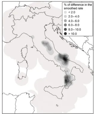
consists of 4427 events and covers approximately the last 1000 years from 1 January 1005 to 28 December 2014. Before using the catalogue, we removed all events not considered main shocks via a declustering filter (Gardner and Knopoff, 1974). This process resulted in a catalogue composed of 1839 independent events, which we denote as the “complete” catalogue. Moreover, to avoid double counting due to the use of two seismicity sources, i.e. the fault sources and the distributed seismicity sources, we re-moved events associated with known active faults from the CPTI15 earthquake catalogue. If the causative fault of an earthquake is known, that particular earthquake does not need to be included in the seismicity smoothing procedure. The earthquake-source association is based on neotecton-ics, palaeoseismology, and seismotectonics papers (see Sup-plement), and in a few cases, macroseismic intensity maps. In Table 2, we listed the earthquakes with known causative fault sources. The differences in the smoothed rates given
Figure 4. Historical earthquakes from the most recent version of the historical parametric Italian catalogue (CPTI15; Rovida et al., 2016), the spatial variations in b values and the polygons defining the five macroseismic areas used to assess the magnitude complete-ness intervals (Stucchi et al., 2011).
by Eq. (2) using the complete and modified catalogues are shown in Fig. 5.
We applied the standard methodology developed by Frankel (1995) to estimate the density of seismicity in a grid with latitudinal and longitudinal spacing of 0.05 . The smoothed rate of events in each cell i is determined as fol-lows: ni= 6jnje 12ij c2 6je 12ij c2 , (2)
where ni is the cumulative rate of earthquakes with
magni-tudes greater than the completeness magnitude Mc in each
cell i of the grid, and 1ij is the distance between the centres of grid cells i and j. The parameter c is the correlation dis-tance. The sum is calculated in cells j within a distance of 3c of cell i.
To compute earthquake rates, we adopted the complete-ness magnitude thresholds over different periods given by Stucchi et al. (2011) for five large zones (Fig. 4).
To optimize the smoothing distance 1 in Eq. (2), we di-vided the earthquake catalogue into four 10-year disjoint learning and target periods from the 1960s to the 1990s. For each pair of learning and target catalogues, we used the prob-ability gain per earthquake to find the optimal smoothing
dis-Figure 5. Differences in percentages between the two smoothed rates computed with Eq. (2) using the complete catalogue and the modified catalogue without events associated with known active faults (TGR model).
tance (Kagan and Knopoff, 1977; Helmstetter et al., 2007). After assuming a spatially uniform earthquake density model as a reference model, the probability gain per earthquake G of a candidate model relative to a reference model is given by the following equation:
G= exp ✓ L L0 N ◆ , (3)
where N is the number of events in the target catalogue and Land L0are the joint log-likelihoods of the candidate model and reference model respectively. Under the assumption of a Poisson earthquake distribution, the joint log-likelihood of a model is given as follows:
L=XNx ix=1 XNy jy=1logp ⇥ (ix, iy), ! ⇤ , (4)
where p is the Poisson probability, is the spatial density, ! is the number of observed events during the target pe-riod, and the parameters ixand iydenote each corresponding
longitude–latitude cell.
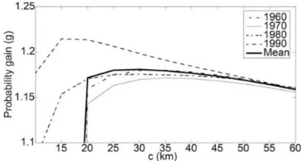
Figure 6 shows that for the four different pairs of learning-target catalogues, the optimal smoothing distance c (the mean curve) ranges from 25 to 40 km. Finally, the mean of all the probability gains per earthquake yields a maximum smoothing distance of 30 km (Fig. 6), which is then used in Eq. (2).
The b value of the GR distribution is calculated on a re-gional basis using the maximum-likelihood method of We-ichert (1980), which allows for multiple periods with varying
Figure 6. Probability gain per earthquake (see Eq. 3) versus corre-lation distance c, used to determine the best radius for use in the smoothed seismicity approach (Eq. 2).
completeness levels to be combined. Following the approach recently proposed by Kamer and Hiemer (2015), we used a penalized likelihood-based method for the spatial estimation of the GR b values based on the Voronoi tessellation of space without tectonic dependency. The entire Italian territory has been divided into a grid with a longitude/latitude spacing of 0.05 , and the centres of the grid cells represent the possible centres of Voronoi polygons. We vary the number of Voronoi polygons, Nv, from 3 to 50, generating 1000 tessellations for each Nv. The summed log-likelihood of each obtained tes-sellation is compared with the log-likelihood given by the simplest model (prior model) obtained using the entire earth-quake data set. We find that 673 random realizations led to better performance than the prior model. Thus, we calculate an ensemble model using these 673 solutions, and the mean bvalue of each grid node is shown in Fig. 4.
The maximum magnitude Mmaxassigned to each node of
the grid, the nodal planes, and the depths have been taken from ESHM13 (Woessner et al., 2015). The ESHM13 project evaluated the maximum magnitudes of large areas of Eu-rope based on a joint procedure involving historical obser-vations and tectonic regionalization. We adopted the lowest value of the maximum magnitude distributions proposed by ESHM13, but evaluating the impact of different maximum magnitudes is beyond the scope of this work.
Finally, the rates of expected seismicity for each node of the grid are assumed to follow the TGR model (Kagan, 2002):
(M)= 0exp( M) exp( Mu)
exp( M0) exp( Mu), (5)
where the magnitude (M) is in the range of M0 (minimum
magnitude) to Mu (upper or maximum magnitude);
other-wise (M) is 0. Additionally, 0 is the smoothed rate of
earthquakes at Mw= 4.5 and = b ln(10).
2.3 Combining fault and distributed sources
To combine the two source inputs, we introduced a distance-dependent linear weighting function, such that the contribu-tion from the distributed sources linearly decreases from 1
to 0 with decreasing distance from the fault. The expected seismicity rates of the distributed sources start at Mw= 4.5,
which is lower than the minimum magnitude of the fault sources, and the weighting function is only applicable in the magnitude range overlapping the MFD of each fault. This weighting function is based on the assumption that faults tend to modify the surrounding deformation field (Fig. 7), and this assumption is explained in detail later in this paper.
During fault system evolution, the increase in the size of a fault through linking with other faults results in an in-crease in displacement that is proportional to the quantity of strain accommodated by the fault (Kostrov, 1974). Un-der a constant regional strain rate, the activity of fault sec-tions arranged across strike must eventually decrease (Nicol et al., 1997; Cowie, 1998; Roberts and Michetti, 2004). Us-ing analogue modellUs-ing, Mansfield and Cartwrigth (2001) showed that faults grow via cycles of overlap, relay forma-tion, breaching, and linkage between neighbouring segments across a wide range of scales. During the evolution of a sys-tem, the merging of neighbour faults, mostly along strike, results in the formation of major faults, which accommo-date the majority of displacement. These major faults are sur-rounded by minor faults, which accommodate lower amounts of displacement. To highlight the spatial patterns of major and minor faults, Fig. 7a and b present diagrams from the Mansfield and Cartwright (2001) experiment in two different stages: the approximate midpoint of the sequence and the end of the sequence. Numerical modelling performed by Cowie et al. (1993) yielded similar evolutionary features for major and minor faults. The numerical fault simulation of Cowie et al. (1993) was able to reproduce the development of a nor-mal fault system from the early nucleation stage, including interactions with adjacent faults, to full linkage and the for-mation of a large thoroughgoing fault. The model also cap-tures the increase in the displacement rate of a large linked fault. In Fig. 7c and d, we focus on two stages of the simu-lation (from Cowie et al., 1993): the stage in which the fault segments have formed and some have become linked and the final stage of the simulation.
Notably, the spatial distributions of major and minor faults are very similar in the experiments of both Mansfield and Cartwrigth (2001) and Cowie et al. (1993), as shown in Fig. 7a–d. Developments during the early stage of major fault formation appear to control the location and evolution of future faults, with some areas where no major faults de-velop. The long-term evolution of a fault system is the conse-quence of the progressive cumulative effects of the slip his-tory, i.e. earthquake occurrence, of each fault. Large earth-quakes are generally thought to produce static and dynamic stress changes in the surrounding areas (King et al., 1994; Stein et al., 1994; Pace et al., 2014; Verdecchia and Carena, 2016). Static stress changes produce areas of negative stress, also known as shadow zones, and positive stress zones. The spatial distributions of decreases (unloading) and increases (loading) in stress during the long-term slip history of faults
Figure 7. Fault system evolution and its implications for our model. (a, b) Diagrams from the Mansfield and Cartwright (2001) analogue experiment in two different stages: the approximate midpoint of the sequence and the end of the sequence. Areas exist around master faults where no more than a single major fault is likely to develop.(c, d) Diagrams from numerical modelling conducted by Cowie et al. (1993) in two different stages. This experiment shows the similar evolutional features of major and minor faults.(e, f) Application of the analogue and numerical modelling of fault system evolution to the fault source input proposed in this paper. A buffer area is drawn around each fault source, where it is unlikely for other major faults to develop, accounting for the length and slip rate of the fault source. This buffer area is useful for reducing or truncating the rates of expected distributed seismicity based on the position of a distributed seismicity point with respect to the buffer zone (see text for details).
likely influence the distance across strikes between major faults. Thus, given a known major active fault geometrically capable of hosting a Mw 5.5 earthquake, the possibility that
a future Mw 5.5 earthquake will occur in the vicinity of the
fault, but is not caused by that fault, should decrease as the distance from the fault decreases. Conversely, earthquakes with magnitudes lower than 5.5 and those due to slip along minor faults are likely to occur everywhere within a fault sys-tem, including in proximity to a major fault.
In Fig. 7e, we illustrate the results of the analogue and nu-merical modelling of fault system evolution and indicate the areas around major faults where it is unlikely that other major faults develop. In Fig. 7f, we show the next step in moving from geologic and structural considerations. In this step, we combine fault sources and distributed seismicity source in-puts, which serve as inputs of the seismogenic model. Fault sources are used to model major faults and are represented by a master fault (i.e. one or more major faults) and its
projec-Figure 8. (a) Annual cumulative MFD and (c) incremental annual MFD computed for the red bounded area in (b). The rates have been computed using (i) the full CPTI15 catalogue; (ii) the declustered and complete catalogue (CPTI15,d, c in the legend) obtained using the completeness magnitude thresholds over different periods of time given by Stucchi et al. (2011) for five large zones; (iii) the distributed sources; (iv) the fault sources; and (v) summing fault and distributed sources (total).
tion at the surface. Distributed seismicity is used to model seismicity associated with minor, unknown, or unmapped faults. Depending on the positions of distributed seismicity points with respect to the buffer zones around major faults, the rates of expected distributed seismicity remain unmodi-fied or decrease and can even reach zero.
Specifically, we introduced a slip rate and a distance-weighted linear function based on the above reasoning. The probability of the occurrence of an earthquake (Pe) with a
Mwgreater than or equal to the minimum magnitude of the fault is as follows: Pe= 8 < : 0, d 1km d/dmax, 1 km < d dmax 1, d > dmax, (6)
where d is the Joyner–Boore distance from a fault source. The maximum value of d (dmax) is assumed to be con-trolled by the slip rate of the fault. For faults with slip rates 1 mm yr 1, we assume d
max= L/2 (L is the length
along the strike, Fig. 2a); for faults with slip rates of 0.3– 1 mm yr 1, d
max= L/3; and for faults with slip rates of
0.3 mm yr 1, d
max= L/4. The rationale for varying dmax
is given by a simple assumption: the higher the slip rate is, the larger the deformation field and the higher the value of dmax. This linear function has been applied around each
fault, without differences between footwall and hanging wall. We applied Eq. (6) to the smoothed occurrence rates of the distributed seismogenic sources. In Fig. 8 we show the an-nual cumulative MFD (Fig. 8a) and incremental anan-nual MFD (Fig. 8c) computed for the red bounded area in Fig. 8b. Because we consider three fault source inputs (red lines in Fig. 8): one using only TGR MFD; one using only CHG MFD; and one using mixed model MFD and because the
MFDs of distributed seismicity grid points in the vicinity of faults are modified with respect to the MFDs of these faults, we obtain three different inputs of distributed seismic-ity (blue lines in Fig. 8). These three distributed seismogenic source inputs differ because the minimum magnitude of the faults is Mw5.5 in the TGR model, but this value depends on
each fault source dimension in the CHG and mixed model. From Mw= 4.5 to Mw= 5.5 the complete CPT15 is fully
described by the MFD of the distributed source input. From Mw= 5.5 to Mw= 6.3 the total MFD (black lines in Fig. 8) computed using only TGR MFD is higher than the MFD computed using only CHG and mixed MFD; this is because the annual rates of occurrences of intermediate-magnitude events obtained with TGR model are higher than the ones obtained with CHG and mixed model, as shown in the incre-mental annual MFD in Fig. 8c. From Mw= 6.4 to Mw= 7.3
the total MFDs computed using only CHG and mixed MFD are higher the total MFD obtained with TGR model.
Our approach allows for incompleteness in the fault database to be bypassed, which is advantageous because all fault databases should be considered incomplete. In our ap-proach, the seismicity is modified only in the vicinity of mapped faults. The remaining areas are fully described by the distributed input. With this approach, we do not define regions with reliable fault information, and the locations of currently unknown faults can be easily included when they are discovered in the future.
3 Results and discussion
To probabilistically obtain ground shaking, we assign the cal-culated seismicity rates, based on the Poisson hypothesis, to
Figure 9. Seismic hazard maps for the TGR and CHG models ex-pressed in terms of peak ground acceleration (PGA) and computed for a latitude–longitude grid spacing of 0.05 . The first and sec-ond rows show the fault source, distributed source, and total maps of the TGR model computed for 10 % probability of exceedance in 50 years and 2 % probability of exceedance in 50 years, correspond-ing to return periods of 475 and 2475 years respectively. The third and fourth rows show the same maps for the CHG model.
their pertinent geometries, i.e. individual 3-D seismogenic sources for the fault input and point sources for the dis-tributed input (Fig. 8). All the computations are performed using the OpenQuake Engine, an open-source software de-veloped recently with the purpose of providing seismic haz-ard and risk assessments (Pagani et al., 2014). Moreover, it is widely recognized within the scientific community for its potential. The ground motion prediction equations (GM-PEs) of Akkar et al. (2013), Chiou and Youngs (2008), Fac-cioli et al. (2010) and Zhao et al. (2006) are used, because these GMPEs were selected in the ESHM13 (Woessner et al., 2015) for active shallow crust. In addition, we used the GMPE proposed by Bindi et al. (2014) and calibrated us-ing Italian data. We combined all GMPEs into a logic tree with the same weight of 0.2 for each branch. Note that these GMPEs use different distance metrics: the Joyner–Boore
dis-Figure 10. An example of the contribution to the total seismic haz-ard level (black line), in terms of hazhaz-ard curves, by the fault (red line), and distributed (blue line) source inputs for one of the 45 602 grid points (L’Aquila, 42.400, 13.400). The dashed lines represent the 2, 10, and 81 % probabilities of exceedance (poe) in 50 years.
tance for Akkar et al. (2013), Bindi et al. (2014), and Chiou and Young (2008) and the closest rupture distance for Facci-oli et al. (2010) and Zhao et al. (2006).
The results of the fault source inputs, distributed source inputs, and aggregated model are expressed in terms of peak ground acceleration (PGA) for exceedance probabilities of 10 and 2 % over 50 years, corresponding to return periods of 475 and 2475 years respectively (Fig. 9).
To explore the epistemic uncertainty associated with the MFDs of fault source inputs, we compared the seismic haz-ard levels obtained based on the TGR and CHG fault source inputs (left column in Fig. 9) using the TGR and CHG MFDs for all the fault sources (details in Sect. 2.1.3). Although both models have the same seismic moment release, the differ-ent MFDs generate clear differences. In fact, for 10 % ex-ceedance probability in 50 years, in the TGR model all faults contribute significantly to the seismic hazard level, whereas in the CHG model, only a few faults located in the cen-tral Apennines and Calabria contribute to the seismic haz-ard level. This difference is due to the different shapes of the MFDs in the two models (Fig. 2c). As shown in Fig. 8, the amount of earthquakes with magnitudes between 5.5 and approximately 6, which are likely the main contributors to these levels of seismic hazard, is generally higher in the TGR model than in the CHG model. At a 2 % probability of ex-ceedance in 50 years, all fault sources in the CHG contribute to the seismic hazard level, but the absolute values are still generally higher in the TGR model.
The distributed input (middle column in Fig. 9) depicts a more uniform shape of the seismic hazard level than that of fault source inputs. A PGA value lower than 0.125 g at a 10 % probability of exceedance over 50 years and lower than 0.225 g at a 2 % probability of exceedance over 50 years
Figure 11. Seismic hazard maps for the mixed model. The first row shows the fault source, distributed source, and total maps com-puted for 10 % probability of exceedance in 50 years, and the sec-ond row shows the same maps but computed for 2 % probability of exceedance in 50 years, corresponding to return periods of 475 and 2475 years respectively. The results are expressed in terms of PGA.
encompass a large part of peninsular Italy and Sicily. Two areas with high levels of ground shaking are located in the central Apennines and northeastern Sicily.
The overall model, which was obtained by combining the fault and distributed source inputs, is shown in the right col-umn of Fig. 9. Areas with comparatively high seismic hazard levels, i.e. hazard levels greater than 0.225 g and greater than 0.45 g at 50-year exceedance probabilities of 10 and 2 % re-spectively are located throughout the Apennines, in Calabria, and in Sicily. The fault source inputs contribute most to the total seismic hazard levels in the Apennines, Calabria, and eastern Sicily, where the highest PGA values are observed.
Figure 10 shows the contribution to the total seismic haz-ard level by the fault and distributed source inputs at a spe-cific site (L’Aquila, 42.400, 13.400). Notably, in Fig. 10, dis-tributed sources dominate the seismic hazard contribution at exceedance probabilities greater than ⇠ 81 % over 50 years, but the contribution of fault sources cannot be neglected. Conversely, at exceedance probabilities of less than ⇠ 10 % in 50 years, the total hazard level is mainly associated with fault source inputs. Moreover, note that the contributions are not based on deaggregation but are computed according to the percentage of each source input in the annual frequency of exceedance (AFOE) value of the combined model.
Figure 11 presents seismic hazard maps for PGA at 10 and 2 % exceedance probabilities in 50 years for fault sources, distributed sources, and a combination of the two. These data were obtained using the above-described mixed model, in which we selected the most appropriate MFD model (TGR or CHG) for each fault (as shown in Fig. 3). The results of
Figure 12. CHG (dotted line), TGR (solid line), and mixed model (dashed line) hazard curves for three sites (see Fig. 13 for the lo-cation): Cesena (red line), L’Aquila (black line), and Crotone (blue line)
this model therefore have values between those of the two endmembers shown in Fig. 9.
Figure 12 shows the CHG, TGR, and mixed model haz-ard curves of three sites (Cesena, L’Aquila, and Crotone, Fig. 13c). As previously noted, the results of the mixed model, due to the structure of the model, are between those of the CHG and TGR models. The relative positions of the haz-ard curves derived from the two endmember models and the mixed model depend on the number of nearby fault sources that have been modelled using one of the MFD models and on the distance of the site from the faults. For example, in the case of the Crotone site, the majority of the fault sources in the mixed model are modelled using the CHG MFD. Thus, the resulting hazard curve is similar to that of the CHG model. For the Cesena site, the three hazard curves overlap. Because the distance between Cesena and the closest fault sources is approximately 60 km, the impact of the fault in-put is less than the impact of the distributed source inin-put. In this case, the choice of a particular MFD model has a limited impact on the modelling of distributed sources. Notably, for an AFOE higher than 10 4, the TGR fault source input
val-ues are generally higher than those of the CHG source input, and the three models converge at AFOE lower than 10 4, as
shown for L’Aquila site. The resulting seismic hazard esti-mates depend on the assumed MFD model (TGR vs. CHG), and for the investigated range of AFOE, especially on the an-nual rates of occurrences of intermediate-magnitude events (5.5 to ⇠ 6.5; see Fig. 8). Therefore, the TGR model leads to the highest hazard values because this range of magnitude (5.5 to ⇠ 6.5) contributes the most to the hazard level.
In Fig. 13, we investigated the influences of the mixed fault source inputs and the mixed distributed source inputs on the total hazard level of the entire study area, as well as the spatial variability. The maps in Fig. 13a show that the
Figure 13. (a) Contribution maps of the mixed fault and distributed source inputs to the total hazard level for three probabilities of exceedance: 2, 10, and 81 %, corresponding to return periods of 2475, 475, and 30 years respectively.(b) Contributions of the mixed fault (solid line), and distributed (dashed line) source inputs along three profiles (A, B, and C inc) for three probabilities of exceedance: 2 % (blue line), 10 % (black line), and 81 % (red line).
contribution of fault inputs to the total hazard level gener-ally decreases as the exceedance probability increases from 2 to 81 % in 50 years. At a 2 % probability of exceedance in 50 years, the total hazard levels in the Apennines and eastern Sicily are mainly related to faults, whereas at an 81 % prob-ability of exceedance in 50 years, the contributions of fault inputs are high in local areas of central Italy and southern Calabria.
Moreover, we examined the contributions of fault and dis-tributed sources along three E–W-oriented profiles in north-ern, central, and southern Italy (Fig. 13b). In areas with faults, the hazard level estimated by fault inputs is generally higher than that estimated by the corresponding distributed source inputs. Notable exceptions are present in areas prox-imal to slow-slipping active faults at an 81 % probability of exceedance in 50 years (profile A), such as those at the east-ern and westeast-ern boundaries of the fault area in central Italy (profile B), and in areas where the contribution of the dis-tributed source input is equal to that of the fault input at a 10 % probability of exceedance in 50 years (eastern part of profile C).
The features depicted by the three profiles result from a combination of the slip rates and spatial distributions of faults for fault source inputs. The proposed approach requires a high level of expertise in active tectonics and cautious expert judgement at many levels in the procedure. First, the seismic hazard estimate is based on the definition of a segmentation model, which requires a series of rules based on observa-tions and empirical regression between earthquakes and the size of the causative fault. New data might make it necessary to revise the rules or reconsider the role of the segmentation. In some cases, expert judgement could permit discrimination among different fault source models. Alternatively, all mod-els should be considered branches in a logic tree approach.
Moreover, we propose a fault seismicity input in which the MFD of each fault source has been chosen based on an anal-ysis of the occurrences of earthquakes that can be tentatively or confidently assigned to a certain fault. To describe the fault activity, we applied a probability density function to the mag-nitude, as commonly performed in the literature: the TGR model, where the maximum magnitude is the upper thresh-old and Mw= 5.5 is the lower threshold for all faults, and
con-Figure 14. Seismic hazard maps expressed in terms of PGA and computed for a latitude–longitude grid spacing of 0.05 based on rock site conditions. The figure shows a comparison of our model (mixed model, left column), the ESHM13 model (FSBG logic tree branch, middle column), and the current Italian national seismic hazard map (MPS04, right column). The same combination of GMPEs (Akkar et al., 2013; Chiou and Youngs, 2008; Faccioli et al., 2010; Zhao et al., 2006; Bindi et al., 2014) were used for all models to obtain and compare the maps.
sists of a truncated normal distribution centred on the maxi-mum magnitude. Other MFDs have been proposed to model the earthquake recurrence of a fault. For example, Youngs and Coppersmith (1985) proposed a modification to the trun-cated exponential model to allow for the increased likelihood of characteristic events. However, we focused only on two models, as we believe that instead of a “blind” or qualita-tive characterization of the MFD of a fault source, future application of statistical tests of the compatibility between expected earthquake rates and observed historical seismic-ity could be used as an objective method of identifying the optimal MFD of expected seismicity. As shown in this anal-yses, fault sources, even if modelled by TGR or CHG MFD, are able to match occurred seismicity for magnitude ⇠ > 5.5 (see for example Fig. 8) and so are complementary to other inputs that model seismicity using area sources or smoothing approaches.
To focus on the general procedure for spatially integrat-ing faults with sources representintegrat-ing distributed (or off-fault) seismicity, we did not investigate the impact of other smooth-ing procedures on the distributed sources, and we used fixed kernels with a constant bandwidth (as in the works of Kagan and Jackson, 1994; Frankel et al., 1997; Zechar and Jordan, 2010). The testing of adaptive bandwidths (e.g. Stock and Smith, 2002a, b; Helmstetter et al., 2006, 2007; Werner et al., 2010; Hiemer et al., 2014) or weighted combinations of both models has been reserved for future studies.
Finally, we compared, as shown in Fig. 14, the 2013 Euro-pean Seismic Hazard Model (ESHM13) developed within the SHARE project, the current Italian national seismic hazard map (MPS04), and the results of our model (mixed model) using the same GMPEs as used in this study. Specifically, for ESHM13, we compared the results to the fault-based haz-ard map (FSBG model) that accounts for fault sources and background seismicity. The figure shows how the impact of our fault sources is more evident than in FSBG-ESHM13, and the comparison with MPS04 confirms a similar pattern, but with some significant differences at the regional to local scales.
The strength of our approach lies in the integration of different levels of information regarding the active faults in Italy, but the final result is unavoidably linked to the quality of the relevant data. Our work focused on presenting and ap-plying a new approach for evaluating seismic hazards based on active faults and intentionally avoided the introduction of uncertainties due to the use of different segmentation rules or other slip rate values of faults. Moreover, the impact of ground motion predictive models is important in seismic haz-ard assessment but beyond the scope of this work. Future steps will be devoted to analysing these uncertainties and evaluating their impacts on seismic hazard estimates.
4 Conclusions
We presented a seismogenic source model for Italy, which summarizes and integrates the fault-based models developed within the last decade (Pace et al., 2006).
The model proposed in this study combines fault source inputs based on over 110 faults grouped into 86 fault sources and distributed source inputs. For each fault source, the maxi-mum magnitude and its uncertainty were derived by applying scaling relationships, and the rates of seismic activity were derived by applying slip rates to seismic moment evaluations and balancing these seismic moments using two MFD mod-els.
To account for unknown faults, a distributed seismicity in-put was applied following the well-known Frankel (1995) methodology to calculate seismicity parameters.
The fault sources and gridded distributed seismicity sources have been integrated via a new approach based on the idea that deformation in the vicinity of an active fault is concentrated along the fault and that the seismic activity in the surrounding region is reduced. In particular, a distance-dependent linear weighting function has been introduced to allow the contribution of distributed sources (in the magni-tude range overlapping the MFD of each fault source) to lin-early decrease from 1 to 0 with decreasing distance from a fault. The strength of our approach lies in the ability to inte-grate different levels of available information for active faults that actually exist in Italy (or elsewhere), but the final result is unavoidably linked to the quality of the relevant data. We think that our seismogenic source model includes significant advances in the use of integrated active fault and seismolog-ical data.
The probabilistically estimated ground shaking maps pro-duced using our model show a hazard pattern similar to that of the current maps at the national scale, but some significant differences in hazard level are present at the regional to local scales (Fig. 13).
Moreover, the impact using different MFD models to de-rive seismic activity rates has on the hazard maps was investi-gated. The PGA values in the hazard maps obtained with the TGR model are higher than those in the hazard maps based on the CHG model. This difference is because the rates of earthquakes with magnitudes from 5.5 to approximately 6 are generally higher in the TGR model than in the CHG model. Moreover, the relative contributions of fault source inputs and distributed source inputs have been identified in maps and profiles in three sectors of the study area. These profiles show that the hazard level is generally higher where fault in-puts are used, and for high probabilities of exceedance, the contribution of distributed inputs equals that of fault inputs.
Finally, the mixed model was created by selecting the most appropriate MFD model for each fault. All data, including the locations and parameters of fault sources, are provided in the Supplement of this paper.
It shall be noted that our new seismogenic source model is not intended to replace, integrate, or assess the current official national seismic hazard model of Italy. While some aspects remain to be implemented in our approach (e.g. the integration of reverse/thrust faults in the database, sensitivity tests for the distance-dependent linear weighting function pa-rameters, sensitivity tests for potential different segmentation models, and fault source inputs that account for fault interac-tions), the proposed model represents advancements in terms of input data (quantity and quality) and methodology based on a decade of research in the field of fault-based approaches to regional seismic hazard modelling.
Data availability. The implementation information of the codes FiSH and OpenQuake is available with the current releases (http:// fish-code.com, last accessed January 2016; https://github.com/gem/ oq-engine, last accessed 30 September 2017). Other details of the fault source input are provided in Valentini et al. (2017) and can be provided on demand.
The Supplement related to this article is available online at https://doi.org/10.5194/nhess-17-2017-2017-supplement.
Competing interests. The authors declare that they have no conflict of interest.
Special issue statement. This article is part of the special issue “Linking faults to seismic hazard assessment in Europe”. It is not associated with a conference.
Acknowledgements. We warmly thank the two reviewers, Lau-rentiu Danciu and Kris Vanneste, and the associated editor, Laura Peruzza, for their detailed and highly instructive reviews. This work was funded by Fondi Dipartimento DiSPUTer (B. Pace, responsible for “ex 60 %” fund) and by the Italian Ministry of Education and Research (MIUR) funded project “High-resolution investigations for the assessment of seismic hazard and risk in the area affected by the earthquake of 6 April 2009” (FIRB-Abruzzo), code: RBAP10ZC8K 006.
Edited by: Laura Peruzza
Reviewed by: Kris Vanneste and Laurentiu Danciu
References
Akinci, A., Galadini, F., Pantosti, D., Petersen, M., Malagnini, L., and Perkins, D.: Effect of Time Dependence on Probabilistic Seismic-Hazard Maps and Deaggregation for the Central Apen-nines, Italy, B. Seismol. Soc. Am., 99, 585–610, 2009.