Lidar observations of mesospheric sodium over Italy (*)
P. DICARLO, V. RIZIand G. VISCONTI Dipartimento di Fisica, Università degli Studi Via Vetoio, Località Coppito, 67010 L’Aquila, Italy (ricevuto il 17 Aprile 1998; approvato il 21 Luglio 1998)
Summary. — We have developed a lidar system for the measurements of the mesospheric atomic sodium (Na) number density profile. The performances and the main characteristics of the system are evaluated showing the first observations: Na number density profiles can be obtained with a resolution of 300 m in altitude and of 200 s in time, the relative uncertainty is between 5% and 10%. These features also allow to discuss the capability of the system to detect the time and space variability of Na density profiles, which is typical of the gravity wave propagation. The preliminary analysis of the sodium profile dynamics along a 7 hours measurement session, started from 19:30UT on 10 April 1997, shows the presence of wave-like perturbations with characteristics typical of propagating gravity waves.
PACS 92.60.Dj – Gravity waves, tides, and compressional waves. PACS 93.85 – Instrumentation and techniques for geophysical research.
1. – Introduction
Meteoric ablations are generally accepted as the dominant source of Na and of the other alkaline metals present in the mesosphere [1]. The Na layer is present at an altitude range from 80 to 110 km and the density peak close to the mesopause (A90 km) is of the order of 103to 104atoms cm23[2].
Since this region is relatively inaccessible to in situ measurements, most studies rely on remote-sensing techniques. One of the most appropriate remote-sensing techniques for the investigation of the mesosphere characteristics is the lidar. The measured backscattered radiation can be discriminated in altitude and on short time periods. For the Na detection, the radiation source of the lidar is a laser with an emission wavelength matching up the frequency of the Na atomic transition from the ground state to the first-excited state. The radiation re-emitted by the Na atoms (resonance scattering) raised at the first-excited state by the laser radiation, is collected with a telescope. The resonance scattering is the most efficient radiation
(*) The authors of this paper have agreed to not receive the proofs for correction.
scattering process in the atmosphere; actually its cross-section is 3 to 4 orders of magnitude larger than the Rayleigh or molecular cross-section. The atomic and molecular densities of the upper atmosphere is so low that the resonance transition linewidth of Na is only Doppler-broadened, therefore the cross-section of the resonance scattering is [3] s(l) 4 2 pe 2 mc f
k
ln ( 2 ) DlD kp exp 2y
2k
ln ( 2 ) (l 2l0) DlDz
2 , (1)where e and m are, respectively, the electron charge and mass, c is the light velocity in vacuum, f (40.655) is the oscillator strength, DlD(41.245 pm) is the Doppler width at half-height and l0(4588.9 nm) is the central wavelength of the transition line. Since resonance scattering is isotropic, the radiation from the Na atoms is emitted with the same probability in all directions, then the differential cross-section can be written:
(
ds (l) OdV)
4 s(l) O4 p .The study of the seasonal, daily and at smaller time scale variations (e.g., sporadic development of very dense narrow layers) of the Na profiles has been investigated with lidar systems [4, 5]. But the Na also is a good tracer to determine mesospheric wave activity, i.e. the perturbations generated by atmospheric tides and gravity waves [6]. The Na atoms are confined in a definite range of altitudes with large densities, and the time scales of the diffusive and chemical processes can be assumed longer than the period of the wave perturbations.
Lidar measurements of the Na layer are conducted in different sites in the world since the late ’60s, but in Southern Europe they are absent. This gap is filled up with the development of the lidar of the University of L’Aquila. In this work we present the features and the capabilities of the system and some preliminary results.
2. – System configuration and performances
This system is situated at 42.35 7N and 13.38 7E, close to L’Aquila (Italy), and is set up in a monostatic configuration. The transmitter part of the system consists of a tunable dye-laser pumped by a frequency-doubled Nd:YAG-laser. The dye-laser uses as dye a solution of Rhodamine 590 and 610 and can be tuned to Na D2 line using a computer-controller grating in the laser cavity. The emitted laser linewidth is 0.05 cm21. The Nd:YAG-laser and dye-laser main characteristics are reported in table I. 1% of laser energy is used to illuminate a hollow cathode Na lamp. The feed-back of the induced opto-Galvanic signal allows to keep the Na D2 line tuning within 0.1 pm during the measurements.
The receiving system uses a Cassegrain telescope coupled via a mechanical chopper and field lens to an interference filter, a photomultiplier and an electronic chain for photon-counting. The characteristics of the receiving system are specified in table II. The electronics allows a sampling frequency of 80 Mhz, but the sampling frequency is kept below 10 Mhz, to be sure that the system is linearly responding. The mechanical chopper, between the telescope and the field lens, prevents saturation effects by the low-altitude molecular backscattering. The chopper is also used to trigger the laser
TABLEI. – Emission system.
Nd: Yang-laser continuum NY80 Repetition rate Energy Divergence Energy stability Pulse width 10 Hz A400 mJ E 0.5 mrad 3.5% 5 ns Dye-laser continuum ND60 Dual grating Precision Divergence Linewidth Stability 2 32400 lines/mm 1 pm E 0.5 mrad 0.05 cm21 0.05 cm21 0C21hours21
TABLEII. – Receiving system. Telescope Primary mirror Total focal length Field of view 50 cm (diameter) 540 cm 0.5 mrad Interferential filter CW FWHM Peak transmission 589.6 nm 2.5 nm A71% PMT Thorn Emi 9202B Spectral response Quantum efficiency Gain S20 21% (peak) 8 Q 104
with the receiving electronics. The data acquisition is performed with an EG&G multi-channel scaler card and a computer. The photon-counting sampling gate is 2 ms large, corresponding to an altitude resolution of 300 m.
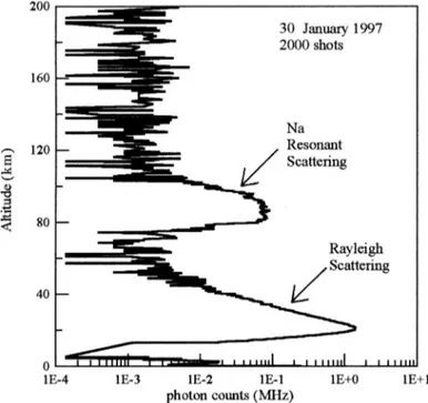
An example of backscattering profile is reported in fig. 1; it has been obtained by accumulating the signal from 2000 laser shots.
Two altitude regions are evident, the lower one (30 to 60 km) is the signature of the molecular backscattering (below 25 km the PMT is obscured by the chopper wheel), while the higher one (between 80 and 110 km) is the resonant signal of Na atoms.
Fig. 1. – Backscattering profile obtained by accumulating the signals from 2000 laser shots.
3. – Data processing
Between 80 km and 110 km, where the Na resonant scattering is dominant, the photons received by the telescope are related to Na density according to [7]
NNa(z) 4hT2(z) seff 4 p A z2an(z)b N0Dz , (2)
where NNa(z) is the photon number coming from the Dz layer which is centred at an altitude z , h is the optical system efficiency, T(z) is the atmospheric transmission factor, seff is the effective cross-section of the resonant backscattering, A is the area of the primary-mirror telescope, N0the photon number emitted by the laser and an(z)b the mean density of the Na atoms in the Dz layer. Accounting the effect of the finite linewidth of the laser, the effective backscattering cross-section is defined:
seff4
s
l s(l) Ne(l) dls
l Ne(l) dl 4 s0DlDk
Dl2 L1 Dl2D!
i 41 6 f expy
24(l02 li) 2ln 2 Dl2 L1 Dl2Dz
, (3)where s04 s(l0) 4pe2fOmc is the peak value of the Na absorption cross-section
(
see eq. (1))
, Ne(l) is the number of photons emitted along the laser line (approximated by a Gaussian shape) at the wavelength l , DlL is the laser linewidth (see table I), DlD is the Doppler width of the Na line, l0 is the central wavelength of Na line, liand fi indicate the wavelengths and the relative strength of the hyperfine structure
of the Na D2 line (i 41, R, 6; l02 li4 20.8476, 20.80513, 20.72881, 1.19498,
1.22031, 1.26275 pm and fi4 0.03125, 0.15625, 0.43750, 0.0625, 0.15625, 0.15625, [8]).
At the lower altitude range, the dominant interaction between laser radiation and atmospheric components is the molecular elastic scattering. Therefore, the lidar equation in this case is [9]
NR(z) 4hT2(z)
g
dsR dVh
p A z2anA(z)b N0Dz , (4)where anA(z)b is the mean density of the atmosphere at z altitude and (dsROdV)pis the
differential cross-section of molecular backscattering.
Coupling eqs. (2) and (4) and scaling the NNa(z) to the NR(z) at an altitude range where the molecular scattering is dominant, it is possible to eliminate the dependence of the detected signals with the laser power fluctuations, the optical transmission of the lower atmosphere and the efficiency of the receiving system
(
i.e. N0, T(z) and h)
. Then, the Na density can be evaluated according toan(z)b 4NNa(z) z2 ( dsROdV)p seffO4 p 1 k i 41
!
k anA(zRi)b NR(zR i) zR i2 . (5)The calibration of the Na resonant backscattering along the zR altitudes is performed between 35 km and 50 km; in this region the aerosol content is negligible, then the contribution of the Mie scattering is neglected; the molecular backscattering signal is
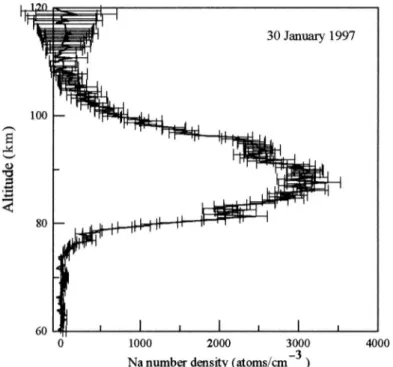
Fig. 2. – The Na number density profile retrieved from the backscattering signal shown in fig. 1. The error bars indicate 3 times the standard deviation.
of the same order as the Na resonant signal and this prevents the possible conse-quences of the signal dynamic; the ratio of the atmospheric transmission functions T2(z
R) OT2(z) is close to one, since both the molecular extinction and the residual absorption between zR and z (the Na layer altitudes) are negligible.
In this sort of measurements the error sources are the uncertainty of the atmospheric density, the statistic fluctuation of the signal and the possible saturation and absorption of the Na atoms. The dominant error is the former and is roughly between 5% and 10% on the relative values of Na number density [10].
In fig. 2 there is an example of a retrieved Na number density profile. It has been obtained from the backscattering signal shown in fig. 1, with an altitude resolution of 300 m, averaging the signals over 200 s time period.
4. – Preliminary analysis
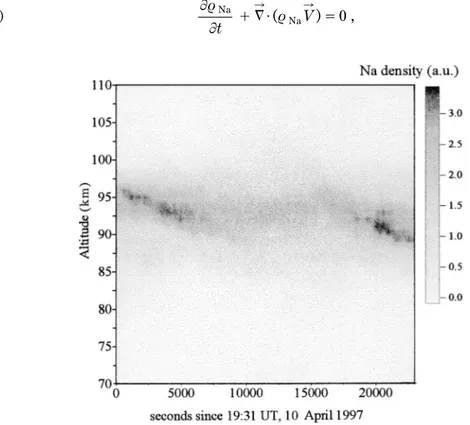
On 10 April 1997 we have collected measurements during a 7 hours long observation session. The time series of the Na density profiles is shown in fig. 3.
Time-dependent perturbations originated by the interaction of the atmospheric wave activity with the Na atoms are quite evident. Actually, at the beginning and the end of this sequence, there is a clear drift of the layer peak. The interaction or response of the Na layer to a wave-like propagating perturbation can be determined solving the continuity equation: ¯rNa ¯t 1 ˜ K Q
(
rNaV K)
4 0 , (6)Fig. 3. – Na number density profiles plotted vs. time, during the 7 hours measurement session. The time and the altitude resolution are, respectively, 200 s and 300 m.
where rNa is Na density and V K
is the velocity field. With the assumption that the diffusion and chemical effect are negligible and the Na layer is horizontal homogeneous, the solution of eq. (6) for a quasi-monochromatic wave disturbance is of the form [6] rNa(z , t) 4 r0 Na
g
z 2gH lnk
1 1 A g 21 expk
z 2 Hl
cos (vt 2kzQ z)l
h
k
1 1 A g 21 expk
z 2 Hl
cos (vt 2kzQ z)l
, (7)where the effect of the perturbation in the argument of r0
Na, which is the function representing the background Na profile, is evident; g is the ratio of the air specific heats, H is the height scale of the atmosphere; A , v and kz are, respectively, the
amplitude, the frequency and the vertical wave number vector of the wave disturbance. If the vertical wavelength of the perturbation is small compared to the full width of the Na layer, eq. (7) can be approximated with the first two terms of a Taylor’s series in power of
[
A Q exp [z/2 H]]
. A simple Fourier transform of this expansion produces a power spectrum that, averaged over a time period t around the time t0for eliminating the v-dependence, looks like [11](8) aNFNa(k) N2b 4NF0Na(k) N21 1
y
gHA 2(g 21)z
2k
g
1 gH 2 1 2 Hh
2 1 (k 2 kz)2l
NF0Na(k 2kz2 iO2 H) N21 2 gHA 2(g 21) sin (vtO2) (vtO2) Re Q Qmk
1 gH 2 1 2 H 1 i(k 2 kz)l
(
F 0 Na(k))
* F 0 Na(k 2kz2 1 O2 H) exp [2ivt0]n
, where FNa(k) and F0Na(k) are the Fourier transforms of the perturbed and unperturbed Na density profiles. This power spectrum is constituted of three terms: the first one gives a low-frequency lobe in the spectrum; the second is the spectral signature of the gravity wave, it is proportional to the square of the wave amplitude and shows a local minimum for k 4kz, i.e., a notch between two peaks; on the other hand,the third term represents the non-linear second-harmonic components of the gravity wave response [11].
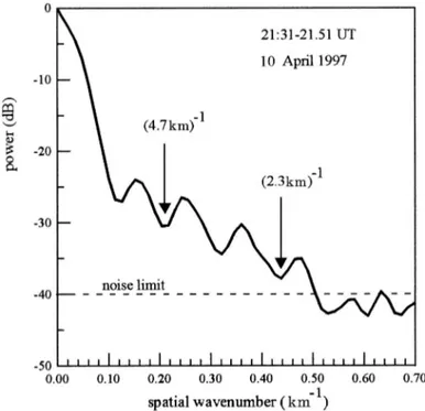
We have applied this analysis in a 20 min time window (between 21:31UT and 21:51UT) of the 10th April 1997 observations. The width of the Na layer (A15 km) sets the maximum vertical wavelength of the wave interacting with Na profiles (i.e. kmin4 0.06 km21); in addition, the altitude resolution (300 m) defines the minimum wavelength (i.e. kmax4 3.3 km21). The obtained mean power spectrum is shown in fig. 4, the features of a wave which interacts with the Na layer are evident: the position of the local minimum between the first two peaks on the side of the low-frequency lobe indicates the gravity wave number (0.21 km21, corresponding to about 4.7 km wavelength). The other notch between the weaker peaks at larger k values corresponds to the local minimum of the third term in eq. (8) (i.e. the non-linear interaction), and its position is at about twice the value of the gravity wave number (0.43 km21).
Fig. 4. – The average spatial power spectra calculated from the Na profiles in a period of 20 min, the wave number corresponding to the first and second harmonic of the interaction between the gravity wave and the Na layer are indicated by the arrows. The dashed line shows the limit set by the noise.
The vertical velocity of the wave can be estimated by looking at the motion of successive peaks in the Na profiles in fig. 3; the apparent phase velocity is 1.7 km/h, thus the wave period (l/c) is about 2.6 hours. This period is Doppler-shifted by the background wind field, and the correction for estimating the intrinsic wave period is not trivial because it depends on mean vertical and horizontal wind velocities.
5. – Conclusions
In this work we report the status and the performances of a lidar system for mesospheric Na sounding. We show that our system, based on standard techniques, has the capabilities for detecting the Na number density profile with an accuracy that allows the study of the small-scale variability of the mesospheric Na content.
Although Gibson-Wilde et al. [12] have well evidenced that there are intrinsic limits on the gravity wave information which can be extracted from Na lidar data, in a preliminary analysis of the 7 hours measurement session, we get the features of wave-like propagating perturbation typical of gravity waves [13]. The system is in routine operation and is now making observation during night. With an extended collection of measurements, we can start a finer data analysis.
R E F E R E N C E S
[1] QIANJ. and Gardner C. S., Simultaneous LIDAR measurements of mesospheric Ca, Na, and temperature profiles at Urbana, Illinois, J. Geophys. Res., 100 (1995) 7453-7461. [2] RICHTERE. S., ROWLETTJ. R., GARDNERC. S. and SECHRISTC. F. jr., LIDAR observation of
the mesospheric Na layer over Urbana, Illinois, J. Atmos. Terr. Phys., 43 (1981) 327-337. [3] ME´GIE G. and BLAMONT J. E., Laser sounding of atmospheric sodium: interpretation in
terms of global atmospheric parameters, Planet. Space Sci., 25 (1977) 1093-1109.
[4] SIMONICHD. M. and CLEMESHAB. R., Resonant extinction of LIDAR returns from the alkali metal layers in the upper atmosphere, Appl. Opt., 22 (1983) 1387-1390.
[5] BEATTY T. J., COLLINS R. L., GARDNER C. S., HOSTETLER C. A. and SECHRIST C. F. jr., Simultaneous RADAR and LIDAR observations of Sporadic E and Na layers at Arecibo, Geophys. Res. Lett., 16 (1989) 1019-1022.
[6] GARDNER C. S. and SHELTON J. D., Density response of neutral atmospheric layers to gravity wave perturbations, J. Geophys. Res., 90 (1985) 1745-1754.
[7] ME´GIE G., BOS F., BLAMONT J. E. and CHANIN M. L., Simultaneous measurements of atmospheric Na and potassium, Planet. Space Sci., 26 (1988) 27-35.
[8] MEASURES M. M. (Editor), Laser Chemical Analysis (John Wiley & Sons, New York) 1988. [9] MEASURES M. M., Laser Remote Sensing-Fundamentals and Applications (John Wiley &
Sons, New York) 1984.
[10] DI CARLO P., Osservazione del sodio nell’alta atmosfera con tecniche LIDAR, Tesi di Laurea, Dipartimento di Fisica, Università degli Studi, L’Aquila, 1997.
[11] GARDNER C. S. and VOELZ D. G., Lidar Studies of Nighttime Na Layer over Urbana, Illinois. Gravity Waves, J. Geophys. Res., 92 (1987) 4673-4694.
[12] GIBSON-WILDE D. E., REID I. M., ECKERMANN S. D. and VINCENT R. A., Simulation of LIDAR measurements of gravity waves in the mesosphere, J. Geophys. Res., 101 (1996) 9509-9522.
[13] LINDZEN R. S., Turbulence and stress owing to gravity wave and tidal breakdown, J. Geophys. Res., 86 (1981) 9707-9714.