Crudu, F., Neri, L., & Tiezzi, S. (2021). Family Ties and Child Obesity in Italy. ECONOMICS AND HUMAN BIOLOGY, 40.
This is the peer reviewd version of the followng article:
Family Ties and Child Obesity in Italy
Published:
DOI:10.1016/j.ehb.2020.100951
Terms of use:
Open Access
(Article begins on next page)
The terms and conditions for the reuse of this version of the manuscript are specified in the publishing policy. Works made available under a Creative Commons license can be used according to the terms and conditions of said license. For all terms of use and more information see the publisher's website.
Availability:
This version is available http://hdl.handle.net/11365/1121496 since 2020-12-02T12:58:09Z
Journal Pre-proof
Family Ties and Child Obesity in Italy<!–<ForCover>Federico Crudu, Laura Neri, Silvia Tiezzi, Family Ties and Child Obesity in Italy,
<![CDATA[Economics and Human Biology]]>,
doi:10.1016/j.ehb.2020.100951</ForCover>–>
Federico Crudu, Laura Neri, Silvia Tiezzi
PII: S1570-677X(20)30221-5
DOI: https://doi.org/10.1016/j.ehb.2020.100951
Reference: EHB 100951
To appear in: Economics and Human Biology
Received Date: 21 January 2020 Revised Date: 25 October 2020 Accepted Date: 16 November 2020
Please cite this article as:{ doi:https://doi.org/
This is a PDF file of an article that has undergone enhancements after acceptance, such as the addition of a cover page and metadata, and formatting for readability, but it is not yet the definitive version of record. This version will undergo additional copyediting, typesetting and review before it is published in its final form, but we are providing this version to give early visibility of the article. Please note that, during the production process, errors may be discovered which could affect the content, and all legal disclaimers that apply to the journal pertain.
Family Ties and Child Obesity in Italy
⇤
1Federico Crudu
† University of Siena and CRENoSLaura Neri
‡ University of SienaSilvia Tiezzi
§ University of Siena 2October 2020
3 Abstract 4This paper examines the impact of overweight family members on weight outcomes
5
of Italian children aged 6 to 14 years. We use an original dataset matching the
6
2012 cross sections of the Italian Multipurpose Household Survey and the
House-7
hold Budget Survey. Since the identification of within-family peer effects is known
8
to be challenging, we implement our analysis on a partially identified model using
9
inferential procedures recently introduced in the literature and based on standard
10
Bayesian computation methods. We find evidence of a strong, positive effect of both
11
overweight peer children in the family and of overweight adults on children weight
12
outcomes. The impact of overweight peer children in the household is larger than
13
the impact of adults. In particular, the estimated confidence sets associated to the
14
peer children variable is positive with upper bound around one or larger, while the
15
confidence sets for the parameter associated to obese adults often include zero and
16
have upper bound that rarely is larger than one.
17
Keywords: child obesity; confidence sets; partial identification; peer effects within the family.
18
⇤We thank three anonymous referees and the Associate Editor Tinna Ásgeirsdóttir, whose comments
greatly improved the paper. Comments from Pamela Giustinelli, Giovanni Mellace, Nicole Hair, and participants at the 2018 Workshop on Institutions, Individual Behavior and Economic Outcomes, Alghero, Italy; the IAAE 2019 Conference, Nicosia, Cyprus; the Nordic Health Economic Study Group (NHESG) 2019, Reykjavik, Iceland; and the 2019 Annual Health Econometrics Workshop, Knoxville TN, USA are gratefully acknowledged.
†Department of Economics and Statistics, University of Siena, Piazza San Francesco, 7/8 53100 Siena,
‡Department of Economics and Statistics, University of Siena, Piazza San Francesco, 7/8 53100 Siena,
§Department of Economics and Statistics, University of Siena, Piazza San Francesco, 7/8 53100 Siena,
1 Introduction
1In the last decades children overweight and obesity prevalence have risen substantially in
2
most countries. According to a new global assessment of child malnutrition by UNICEF
3
(UNICEF, 2019) the most profound increase has been in the 5-19 age group, where the
4
global rate of overweight increased from 10.3% in 2000 to 18.4% in 2018.
5
Identifying the determinants of child obesity is a compelling issue since obesity is not
6
only a direct threat for children’s health and a cost to society, but also has documented
7
consequences for adult life, such as effects on health (Llewellyn et al., 2016), on self-esteem,
8
body image and confidence, and on wages (Schwartz et al., 2011).
9
It is recognised that child consumption decisions are affected by those of their peers
10
(Dishion & Tipsord, 2011) and that peer effects are more pronounced in children than in
11
adolescents (Nie et al., 2015). While classroom or friends peer effects have been found to
12
explain childhood and adolescents obesity (Asirvatham et al., 2014; Gwozdz et al., 2015;
13
Nie et al., 2015), the role of within-the-family peers, e.g. interaction with other overweight
14
and obese peer children in the family, as a determinant of child overweight and obesity has
15
not yet been investigated.1 16
In fact, within-the-family social interaction could be an important determinant of child
17
obesity, because children spend most of their time in the family environment. A likely
18
driving mechanism is imitation. Research in experimental psychology (Zmyj, Ascherslebel
19
et al., 2012; Zmyj, N. Daum et al., 2012; Zmyj & Seehagen, 2013) postulates that prolonged
20
individual experience with peers leads children to imitate peers more than adults. Children
21
imitate familiar behaviour for social reasons, such as identification with the role model or
22
to communicate likeness. Adults are the natural model on which children rely in unfamiliar
23
situations while age is an important indicator of likeness. With prolonged contact with
24
peers (i.e. children in the same age group), children are more likely to imitate behaviour
25
1An exception is the famous study by Christakis & Fowler (2007) focusing on adults. One of their main
findings was that, among pairs of adult siblings, if one sibling became obese, the chance that the other would become obese increased by 40% and that if one spouse became obese, the likelihood that the other spouse would also become obese increased by 37%.
from them than from adults, because they learn to trust their peers and to refer to them
1
for learning also in unfamiliar situations. In this case imitation serves a cognitive function:
2
prolonged contact with peers leads children to believe that peers are as competent as
3
adults, i.e. a reliable model. Since children plausibly spend extended periods of time with
4
family members, such prolonged contact is reflected in increased levels of peers imitation.
5
If imitation is the driving mechanism through which within-the-family social interaction
6
affects child obesity, then the impact of peer children in the family should be larger than
7
the impact of adults.
8
The purpose of this paper is to investigate whether the presence of other overweight/obese
9
family members, i.e. children in the same age group and adults, has a positive and
signi-10
ficant effect on the probability of a child being overweight/obese. To address this research
11
question we use a unique cross-section of Italian households containing detailed
inform-12
ation on families’ structure, composition, habits, and weight outcomes. We estimate a
13
binary choice model where the dependent variable is a binary indicator for each child
be-14
ing overweight or obese or not. The main explanatory variables of interest are the share
15
of other overweight or obese children in the same age group in the family, and the share of
16
overweight or obese adults in the family.
17
To assess the impact of children in the same age group and family (our peer effect), we
18
use a narrow peer-group definition that includes all children aged 6 to 14 years belonging
19
to the same family whether siblings or not. While assessing the impact of adults does not
20
pose particular challenges, within-the-family peer effects are particularly difficult to identify.
21
Narrow definitions of the peer group, such as ours, have been found to be more endogenous
22
than broad ones, because of shared common traits, habits and environments that may cause
23
simultaneity effects (Black et al., 2017; Trogdon et al., 2008). A shared environment also
24
complicates the problem of controlling for unobserved fixed effects, because the latent
25
heterogeneity that may affect the weight outcome of each child is likely to affect the weight
26
outcome of the other children in the same family and age group.
27
In order to provide some further intuition on the mechanics of our problem and on
28
the potential causal interpretation of the model, let us consider a simple directed acyclic
1
graph (DAG) (see Figure 1) to represent the relationship among the main variables of
2
our model. Our main problem is to study the relationship of the peer effect variable
3
(P eer) on the obesity score (Obesity) of a given child in the family. We may reasonably
4
conjecture that Obesity would depend on Exogenous and Contextual variables as well
5
as other Unobserved characteristics. Identifying peer effects may be complicated for a
6
number of reasons. First, in the context of a group of siblings the assignment to a given
7
family is nonrandom and it would reasonably depend on the characteristics of the parents.2 8
Second, genetic and behavioral characteristics may be important to determine whether an
9
individual is obese or not. The former set of characteristics more than the latter may
10
be difficult to observe. However, there may exist some suitable proxy variables that may
11
work as mediators between the Unobserved variables and P eer, these may be physical
12
characteristics such as adults’ weight and height (or BMI) and history of chronic diseases.
13
If this is the case, by controlling for the Exogenous effects and the Contextual effects in
14
Figure 1 we may be able to identify the causal relation between P eer and Obesity. The
15
assumption that Unobserved does not affect P eer may be difficult to maintain in some
16
applications. In the analysis of peer effects in the classroom context, for example, one would
17
reasonably assume that such unobserved factors may be related to family characteristics
18
and in particular to teacher quality. In this case, i.e. if Unobserved affects P eer, identifying
19
the causal effect of P eer on Obesity may be impossible.
20
2The implicit assumption here is that family members are consanguineous.
Figure 1: This DAG shows the causal relationship between Obesity and the peer effect variable P eer. In this model, controlling for Exogenous and Contextual allows one to identify the causal effect of P eer on Obesity.
Due to the narrow peer group and to the structure of the data, however, our
identific-1
ation problem remains hard to solve. We resort to a binary choice model and to partial
2
identification results for such models (see Section 4 for further details on the identification
3
problem and, e.g., Blume et al., 2011; Brock & Durlauf, 2001, 2007).
4
Inferential procedures for partially identified models are often rather complicated.
How-5
ever, the method we use in this paper, introduced by Chen et al. (2018), is computationally
6
rather simple and boils down to calculating confidence sets for the parameters of interest
7
by means of standard Bayesian computation methods. Consistently with the hypothesised
8
driving mechanism, we find evidence of a strong, positive and statistically significant effect
9
of overweight and obese peer children and a smaller positive and generally statistically
10
significant effect of overweight and obese adults in the family on children’s obesity.
11
Our contribution to the existing literature is threefold. First, to our knowledge this is
12
the only paper studying the causal role of within-family peer effects on obesity as a relevant
13
health outcome. If peers in the family have important influences on child weight outcomes,
1
policies affecting one child in the family may have beneficial effects on the other children
2
as well as a social multiplier effect.
3
Second, as stressed by Blume et al. (2011), the literature on partial identification for
4
social interaction models has evolved separately from that on the estimation of partially
5
identified models via bounds initiated by Tamer (2003) and used in industrial organization.
6
This paper is an attempt to integrate these two bodies of literature in a very specific
7
context.
8
Finally, this is the only study on social interaction and child obesity in Italy. Obesity
9
rates are low in Italy compared to most OECD countries, but the picture is different for
10
children. According to the fifth wave of the Italian Surveillance System Okkio alla
Sa-11
lute, in 2016 the prevalence rates of overweight (including obese) and obese primary school
12
children were 30.6% and 9.3%, respectively, with southern regions displaying higher rates
13
than northern regions (Lauria et al., 2019). The Surveillance System Okkio alla Salute
14
(http://www.epicentro.iss.it/okkioallasalute/) monitors overweight and obesity of
15
Italian children in primary schools (6-11 years of age). The System, promoted and financed
16
by the Italian Ministry of Health, was started in 2007 and participates in the World Health
17
Organization (WHO) European Childhood Obesity Surveillance Initiative (COSI). In
ad-18
dition, family ties are culturally strong in Italy which makes social interaction within the
19
family a particularly interesting issue to explore.
20
The remainder of the paper unfolds as follows. Section 2 summarizes the literature.
21
Section 3 describes the data. Section 4 discusses our identification strategy. Section 5
22
presents the estimation methods and main results. Section 6 concludes. Finally, the
Ap-23
pendix contains a description of statistical matching, results for the full sets of parameters
24
and the results of the robustness checks.
2 Child Obesity and Peer Effects
1The main recognized cause of the rise in child obesity is an imbalance between calorie intake
2
and calorie expenditure. There is a vast literature on the factors driving this imbalance.
3
One strand has addressed the relationship between maternal employment and child obesity
4
in many developed countries. Maternal employment is usually associated with higher child
5
weight outcomes, because employed mothers may have less time to pay attention to their
6
children’s diet (Cawley & Liu, 2012; Champion et al., 2012; Fertig et al., 2009; Gaina et al.,
7
2009; García et al., 2006; Greve, 2011; Gwozdz et al., 2013; Liu et al., 2009; Morrill, 2011,
8
to cite only a few). Overall, these studies find empirical evidence of a positive relationship
9
between maternal employment and childhood obesity. However, there is no evidence of such
10
positive relationship in Italy. In Italy there is a female labor force participation divide and
11
a child obesity divide. The South has a very low female labor force participation compared
12
to the North, but child obesity prevalence is much higher in the South compared to the
13
North (Brilli et al., 2016).
14
A related factor is the increasing use of non-parental child care (informal care by a
15
relative, care by a baby-sitter and centre-based care) which may increase the likelihood
16
of obesity (Herbst & Tekin, 2011; Hubbard, 2008). The growing use of non-parental care
17
may play a crucial role in shaping children’s habits through the quality of the food offered
18
and the level of physical activity. Herbst & Tekin (2011) find that centre-based care is
19
associated with large and stable increases in BMI throughout its distribution, while the
20
impact of other non-parental arrangements appears to be concentrated at the tails of the
21
distribution.
22
A strand of literature, initiated by Christakis & Fowler (2007), has emerged in health
23
economics that addresses the influence of social interaction, particularly of peers, on health
24
status. In their seminal paper Christakis & Fowler (2007) conducted a study to determine
25
whether adult obesity might spread from person to person. Their starting point was that
26
people embedded in social networks are influenced by the behaviours of those around
27
them such that weight gain in one person might influence weight gain in others. That
1
study focused on social interaction among adults. A follow up study by the same authors
2
(Fowler & Christakis, 2008) produced evidence of person-to-person spread of obesity also
3
in adolescents.
4
Powell et al. (2015) has identified social contagion, i.e. the phenomenon whereby the
5
network in which people are embedded influences their weight over time, as one of the
6
social processes explaining the rise of adult overweight and obesity. The general finding
7
is that weight-related behaviours of adolescents are affected by peer contacts (Fowler &
8
Christakis, 2008; Halliday & Kwak, 2009; Mora & Gil, 2013; Renna et al., 2008; Trogdon
9
et al., 2008). These studies take adolescents as the relevant age group and the classroom
10
or friends as the relevant network. Much less is known about children as the relevant age
11
group and the family as the relevant network.3 12
To the best of our knowledge only four studies, besides ours, analyse peer effects among
13
children as the relevant population, and child obesity as the relevant outcome. Asirvatham
14
et al. (2014) study peer effects in elementary schools using measured obesity prevalence
15
for children cohorts within schools and using a panel dataset at grade level from Arkansas
16
public schools. They found that changes in the obesity prevalence at the highest level
17
are associated with changes in obesity prevalence at lower grades and the magnitude of
18
the effect is greater in kindergarten to fourth-grade schools than in kindergarten to
sixth-19
grade schools. Nie et al. (2015) analyse peer effects on obesity in a sample of 3 to 18
20
years old children and adolescents in China. Peer effects are found to be stronger in rural
21
areas, among females and among individuals in the upper end of the BMI distribution.
22
Gwozdz et al. (2015) analyse peer effects on childhood obesity using a panel of children
23
aged 2 to 9 from eight European countries. They show that, compared to the other
24
European countries in the sample, peer effects are larger in Spain, Italy and Cyprus. These
25
studies adopt a fairly broad definition of peer effects, either peers at the same grade level
26
3Nie et al. (2015) report that most of the empirical literature on peer effects and obesity refers to
adolescents or adults and uses US data.
within a school or children in a similar age group within a specific community. Finally,
1
Yajuan et al. (2016) estimate peer effects on third grade students’ BMI from a childhood
2
obesity intervention program targeted at elementary schools students in Texas. Peer effects
3
were found for students aged 8-11, with gender differences in the psychological and social
4
behavioral motivations.
5
None of the above studies focuses on the family as the relevant peer group.
6
The literature on the causal role of siblings on children’s outcomes is recent and growing.
7
This literature has focused on the effects of sibling health status on educational outcomes
8
(Black et al., 2017; Fletcher et al., 2012), on the effect of early health shocks on child
9
human capital formation (Yi et al., 2015), on the effects of teen motherhood on their
10
siblings’ short and medium term human capital development (Heissel, 2017, 2019), on the
11
effect of siblings on educational choices and early career earnings (Dustan, 2018; Joensen &
12
Nielsen, 2018; Nicoletti & Rabe, 2019; Qureshi, 2018), and on the effects of health shocks
13
to individuals on their family members consumption of preventive care (Fadlon & Nielsen,
14
2019).
15
Our study contributes to the latter strand of literature considering children as the
16
relevant population and obesity as the relevant health outcome. We conjecture that the
17
mechanism through which the peer effect plausibly operates is via imitation of good and
18
bad behaviours such as eating habits.
19
3 Data and Matching
20The choice of the family as the relevant network to analyse peer effects complicates the
21
problem of controlling for unobserved fixed effects. Thus, the amount of available
inform-22
ation is a crucial issue in our case. Studies of peer effects and childhood obesity usually
23
include information on economic characteristics of the household, such as income, in
ad-24
dition to personal and socio-demographic information, because low-income individuals are
25
more likely to be obese than those with high-income (Trogdon et al., 2008). Moreover, the
26
relationship between income and weight is reported to vary by gender, race/ethnicity and
1
age.4 Lacking a single Italian cross section containing individual weight outcomes, detailed 2
family characteristics and socio-economic variables, we used statistical matching (SM) to
3
match two datasets. The first is the 2012 cross section of the Multipurpose Survey on
4
Households: Aspects of Daily Life (MSH) containing detailed information on family
char-5
acteristics and the weight outcome of each member. The second is the 2012 cross section of
6
The Household Budget Survey (HBS) covering details of current and durable expenditures.
7
Both surveys are conducted by the Italian National Statistical Institute (ISTAT).
8
The MSH for the year 2012 is a large nationally representative sample survey covering
9
19,330 households and 46,463 family members, including children aged 6 to 14 years.5 10
The questionnaire, administered by paper and pencil, contains three blocks of questions: a
11
general questionnaire on individual characteristics of the first six members of the household;
12
a family questionnaire collecting information about household habits and lifestyles; a diary
13
of health and nutritional information for each member of the household. For children and
14
adolescents aged 6-17 a binary indicator for whether the child is overweight or obese is also
15
included. Identification of a child as overweight or obese is based on BMI threshold values
16
for children aged 6 to 17 developed by Cole et al. (2000) and adopted by the International
17
Obesity Task Force (IOTF). The MSH does not contain information on expenditures that
18
could be important covariates in our empirical model. We obtain this information from
19
the 2012 cross section of the HBS which includes monthly consumption expenditures of
20
22,933 Italian households. ISTAT uses a weekly diary to collect expenditure data on
21
frequently purchased items and a face-to-face interview to collect data on large and durable
22
expenditures. Current expenditures are classified into about 200 elementary goods and
23
services.
24
The survey also includes detailed information on household structure and socio-demographic
25
4Food Research and Action Center: http://frac.org/obesity-health/relationship-poverty
-obesity.
5According to both the HBS and the MSH a family or household is defined as the set of cohabiting
persons linked by marriage or kinship ties, affinity, adoption, guardianship or affection.
characteristics (such as regional location, household size, gender, age, education and
em-1
ployment condition of each household member). For both surveys, annual samples are
2
drawn independently according to a two-stage design.6 In addition to having a large set 3
of variables in common, the two surveys share many characteristics such as the target
4
population, sampling method, geographic frame and data collection procedure. These
5
common characteristics allow us to use SM as an ideal method for combining information
6
on households’ quality of life and child weight outcomes with information on households’
7
consumption expenditures.7 8
The sample under analysis includes 3,906 observations. The unit of analysis is defined
9
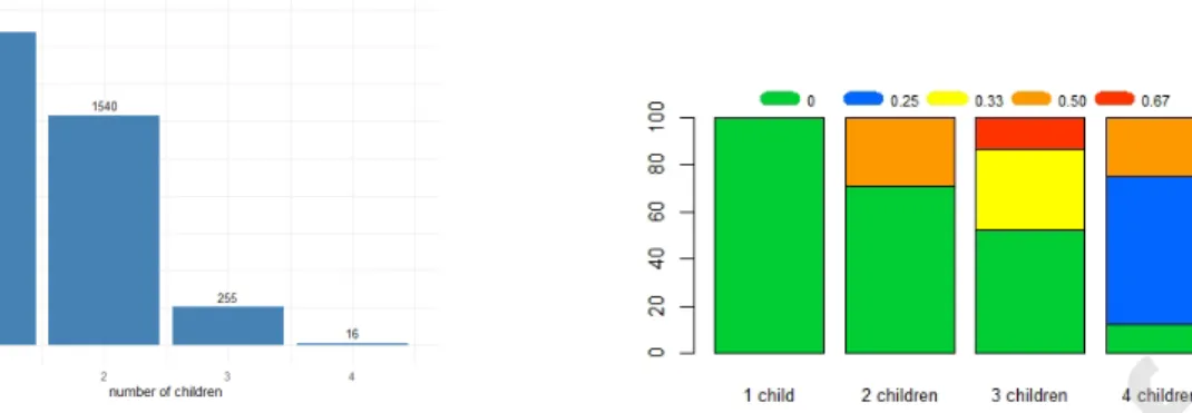
as child aged between 6 and 14 years: the barplot in Figure 2 panel (a) displays how
10
children are distributed across households. The 3,906 children involved in the analysis are
11
distributed across 2,954 households. As shown in Figure 2 panel (a), 2,095 children have
12
no siblings in the target age group: 6 to 14 years; 770 households have two children in
13
the same age group, for a total number of children equal to 1,540; 85 households have
14
three children in the same age group, thus the total number of children is 255; finally, 4
15
households have four children in the target age group, for a total amount of children equal
16
to 16.
17
For each individual, a rich set of covariates is available. Table 1 shows summary
stat-18
istics of the relevant variables in the final SM dataset. We distinguish five sets of variables:
19
individual characteristics of children (panel A), household characteristics (panel B), in some
20
cases related to the household’s reference person (RP), behavioural variables (panel C),
21
proxies for genetic characteristics (panel D), regional variables (panel E). More specifically,
22
the individual characteristics are the child overweight/obesity indicator (our dependent
23
variable), gender and age for each child in the household. There are 1,141 overweight/obese
24
children out of 3,906, thus overweight/obese children account for 29% of children aged 6-14
25
6Details on the sampling procedure used to collect data in both surveys can be found in: ISTAT (2012)
Indagine Multiscopo sulle Famiglie, aspetti della Vita quotidiana, Anno 2012, for the MSH survey; and in ISTAT (2012) File Standard-Indagine sui Consumi delle Famiglie-Manuale d’uso, anno 2012, for the HBS survey. Downloadable at http://www.istat.it/it/archivio/4021.
7SM of the two data sets is detailed in Appendix A.
Table 1: Summary statistics.†
Mean S.d. Min. Max. Obs.
A. Individual characteristics
Child obesity 0.292 0.455 0 1 3,906
Age 9.987 2.595 6 14 3,906
Gender (male) 0.495 0.500 0 1 3,906
B. Household characteristics
Share of other overweight/obese children 0.072 0.174 0 0.667 3,906
Share of overweight/obese adults 0.420 0.351 0 1 3,906
Household size 4.120 1.018 2 11 3,906
Children born of previous marriage 0.007 0.086 0 1 3,906
Monthly expenditure (Euro) 2,131 1,346 237 16,998 3,906
Employed RP 0.813 0.390 0 1 3,906
Student or housewife RP 0.053 0.225 0 1 3,906
Retired or other emp. status RP 0.023 0.150 0 1 3,906
Mother’s education (Master) 0.126 0.331 0 1 3,906
Mother’s education (Bachelor) 0.029 0.169 0 1 3,906
Mother’s education (High School) 0.348 0.476 0 1 3,906
Mother’s education (Junior High) 0.412 0.492 0 1 3,906
Mother’s education (Primary School) 0.068 0.252 0 1 3,906
Central or northern region 0.578 0.494 0 1 3,906
C. Behavioral characteristics
Siblings (regularly) practising sport 0.176 0.244 0 0.75 3,906
Siblings lunch at home 0.186 0.246 0 0.75 3,906
Siblings walking to school 0.089 0.193 0 0.75 3,906
Siblings TV watching every day 0.810 0.317 0 1 3,906
Parents soda drinks 0.155 0.362 0 1 3,906
Parents smoking 0.372 0.483 0 1 3,906
Children average fruit portions 1.125 0.754 0 5.5 3,906
Adults average fruit portions 1.147 0.778 0 5.5 3,906
D. Proxies for genetic characteristics
Mean adult weight (kg) 70.676 9.159 35.5 117.5 3,906
Mean adult height (cm) 168.959 5.694 110 193 3,906
Chronic disease 0.251 0.439 0 1 3,906
Diabetes 0.034 0.181 0 1 3,906
E. Other characteristics
CPI (2010=100) 106.022 0.614 104.6 108.1 3,906
% obese adults by region 24.954 5.476 17.7 36.1 3,906
†This table includes summary statistics on individual characteristics of children (panel A), household
characteristics (panel B), in some cases related to the household’s reference person (RP), behavioural variables (panel C), proxies for genetic characteristics (panel D), regional variables (panel E).
years. The children’s mean age is 10 and the percentage of male children is 49.5%.
1
(a) Distribution of children across families (6 age 14). (b) Conditional distribution of obese/overweight children across families (6 age 14).
Figure 2: Children’s distribution and share of obese children
The peer effect variable is defined as the share of other (overweight and obese) children
2
in the family (excluding the child considered). This variable, mg i, is computed as the ratio 3
between the number of obese children in family g excluding the reference child i, nO g i, and 4
the total number of children in the family, ng. Hence, 5
mg i =
nO g i
ng
where, in our data set, 1 ng 4, 0 nOg i 3 and 0 mg i 2
3. The minimum 6
value of the variable corresponds to two different cases. The first case occurs when child i
7
has no siblings and the second occurs when child i has no obese siblings. The maximum
8
value occurs when there are two out of three obese children in the family.
9
Figure 2 (panel b) shows the conditional distribution of the share of other obese/overweight
10
children in the family given the number of children in the target age group within the
fam-11
ily. Of course, if the reference child has no siblings, the share is zero. As to the children
12
having siblings in the age group 6-14, we can observe the following picture: the number
13
of children in families with two children in the target age group is 1,540, 71% of them
14
has a sibling with normal weight (share = 0) and 21% has an obese/overweight sibling
15
(share = 1/2 = 0.5); the number of children in families with three children in the target
1
age group is 255, 52% the of them has siblings with normal weight (share = 0), 33% of
2
them has one obese/overweight sibling (share = 1/3 = 0.33), and the remaining 13% has
3
two obese/overweight siblings (share = 2/3 = 0.67). Finally, the number of children in
4
families with four children in the target age group is 16, 12.5% of them has normal weight
5
siblings (share = 0), 62.5% has 1 obese/overweight sibling (share = 1/4 = 0.25) and 25%
6
of them has two obese/overweight siblings (share = 2/4 = 0.5).
7
Further characteristics shown in Table 1 include the share of overweight and obese adult
8
family members (42%), household size (4 on average) and a dummy for children born from
9
a previous marriage, the employment status of the RP (three dummies for whether the
10
household RP is employed, a student or housewife, retired or in other employment positions
11
(e.g. military, unable to work, detained)), dummies for the level of education of the mother
12
(five dummies for whether the mother holds a Master’s degree, a Bachelor’s degree, has
13
attended High School, Junior High, or only Primary School) and a dummy for whether the
14
household lives in a central or northern Italian region. In addition, we include monthly
15
current expenditure, whose average value is 2,131 Euros. This variable is important as
16
it captures contextual effects and we conjecture that its support (237 - 16,998 Euros) is
17
sufficiently large to ensure that a nonlinear relationship with the share of obese children
18
in the family (the endogenous effect) exists. We also include a set of variables capturing
19
behaviors of siblings in a wider age group (6 to 18 years) compared to the target age group,
20
because older siblings could influence the behaviours of younger ones. Such variables
21
include the share of siblings (excluding the child under consideration) aged between 6
22
and 18 watching TV every day, having lunch at home, practicing physical activities on a
23
regular basis and walking to school, dummies for whether the parents consume soda drinks
24
or smoke. We also include the child’s daily average fruit portions and the adults daily
25
average fruit portions. As proxies for the genetic variables we use the mean height and
26
weight of the adult members of the family and two dummy variables for whether the RP
27
or her spouse suffer from a chronic disease or diabetes. Finally, we use two additional
28
variables at the regional level: the 2012 consumer price index (CPI) (2010=100) and the
1
percentage of obese adults by region in 2012.
2
4 Identification
3Our aim is to assess whether the presence of other overweight/obese family members,
4
i.e. children in the same age group and adults, has a positive and significant effect on
5
the probability of a child being overweight/obese. If imitation behaviour is the driving
6
mechanism we also expect that the impact of overweight/obese peer children in the family
7
is larger than the impact of overweight/obese adults. We use a narrow peer-group definition
8
that includes all children aged 6 to 14 years belonging to the same family (whether siblings
9
or not). Narrow definitions of peer groups have been found to be more endogenous than
10
broad ones. In particular Trogdon et al. (2008) report that broader measures of social
11
networks (e.g. grade-level peer groups) are more exogenous than narrow ones (e.g. children
12
in the same family) as they are likely to be determined by different causal mechanisms.
13
While grade-level peer effects may be driven by BMI related social norms and body image
14
concerns, family-level peer effects may also operate through additional channels such as
15
the influence of diets, habits and physical activities. Christakis & Fowler (2007) showed
16
that the influence of the weight of friends, family members and neighbours decreases with
17
increasing degrees of separation from the person under investigation. Despite the large
18
empirical literature on social interaction in a variety of contexts, identifying such effects
19
remains a formidable challenge.
20
Let us consider the notation and the definitions in Brock & Durlauf (2007). We assume
21
that individual binary weight outcomes are determined by five sets of factors:
22
(i) observable individual-specific characteristics known also as the exogenous effects,
23
measured by an r-vector Xi; 24
(ii) unobservable individual characteristics summarized by a scalar "i; 25
(iii) observable group characteristics, measured by an s-vector Yg; these are known as con-1
textual effects and may directly influence individual decisions: for example, peers’
2
characteristics such as parents’ income, education or occupation may influence
chil-3
dren’s weight;
4
(iv) unobservable (to the econometrician) group characteristics, measured by a scalar
5
↵g that may affect individual outcomes; these are known as correlated effects: for 6
example, genetic characteristics may affect the weight of all children in the same
7
family;
8
(v) the average outcome in the peer group excluding the child under consideration, mg i. 9
It is a measure of the share of obese children in the family that could affect each
10
individual outcome (see Section 3 for the definition of mg i). 11
Thus, our model of social interaction can be described as
!i = k + c0Xi+ d0Yg+ Jmg i + "i+ ↵g (1)
where !i is a binary indicator that takes value one if, according to a BMI score, individual 12
i is overweight/obese and zero otherwise. One important advantage of using a binary
13
choice model is that, under a large support on Yg, the data reveal a non-linear relationship 14
between mg i and Yg. This implies that the so-called reflection problem Manski (1993) 15
does not arise in the binary choice case 8. 16
Identification in binary choice models of social interaction has been thoroughly explored
17
in Brock & Durlauf (2007) (see also Blume et al., 2011, for a survey). In their baseline
18
result, with ↵g = 0and random assignment, the model parameters are identified up to scale 19
and the reflection effect that typically characterizes linear-in-means models is not present.
20
The main argument relies on the support of the contextual effects Yg to be sufficiently 21
8A reflection problem arises when the dependent variable (weight outcome of child i) and the
explan-atory variable of interest (peer variable mg i) are simultaneously determined, causing an endogeneity issue.
large to establish a nonlinear relationship with mg i. In addition to that, they derive 1
identification results also for the case of non random assignment provided that ↵g = 0. 2
With respect to our context, the assumption of random assignment is very difficult to
3
justify. Since individuals within a group are consanguineous with high probability, their
4
assignment to a given group g depends on common genetic traits. Unfortunately, our
5
data set does not contain any explicit information on the genetic factors that determine
6
obesity in the group. However, we may proxy it with mean adult height and weight in
7
the household and by adding two dummy variables for whether the household head or
8
her spouse suffers from a chronic disease or diabetes. We can conjecture that our proxies
9
capture sufficient information from the fixed effect to guarantee identification. However,
10
we cannot be sure that all relevant assumptions are met.
11
When point identification is not possible, Brock & Durlauf (2007) describe a number
12
of situations where at least partial identification can be achieved. In particular, they
13
prove that under non random assignment, provided that ↵g = 0 and the support on Yg is 14
sufficiently large to rule out the reflection problem, J > 0 and J is large enough to produce
15
multiple equilibria. This means that group g may coordinate on an equilibrium expected
16
average choice level other than the largest of the possible equilibria associated with it
17
while another group g0 may coordinate on an equilibrium other than the lowest possible 18
expected average choice level among those it could have attained. One of the situations
19
where this may happen is the case of assortative matching, where higher group quality
20
is related to higher individual quality. In our context, this may refer to the case where
21
individuals within a specific group share common genetic traits or the same eating habits.
22
It is, though, important to stress that the multiple equilibrium results in Brock & Durlauf
23
(2007) hold for large groups. In particular, Krauth (2006) suggests that multiplicity of
24
equilibria for small groups may happen for lower threshold values of J.
25
We adopt Brock & Durlauf (2007) approach to (partial) identification. In the empirical
26
exercise we need to accommodate the large support assumption on Yg. More specifically, 27
we consider two cases. In the first case the variable with large support is the log of
28
expenditures. The second specification includes also average adult weight and average
1
adult height. It is interesting to notice, though, that there seem to be no clear theoretical
2
guidelines on how many variables with large support would be necessary to avoid the
3
reflection effect (see e.g. Blume et al., 2011, p. 907).
4
Dealing with unobservable heterogeneity in the context of social interaction models is
5
generally a very challenging task since, as suggested in Blume et al. (2011), "i and ↵g are 6
undertheorized.9 Nonetheless, there are still a number of approaches that can be exploited 7
when sufficient information is available. The most problematic issue in our setting is
8
how to deal with the group fixed effects ↵g. The simplest solution here is just to define 9
↵g = d0Yg+ Jmg i (Blume & Durlauf, 2006). This is, we approximate ↵g with observables 10
and change the number of variables in Yg to assess the stability of the estimates. Our 11
model will include a large number of group characteristics that may reasonably determine
12
obesity and that are either related to genetic factors or to behavioural factors.10 13
Direct estimation of ↵g via group dummies would be impossible in our context due 14
to the large number of families (2,954) compared to the number of individuals (3,906).
15
We could however identify a restricted number of groups by clustering families with
com-16
mon characteristics. The resulting number of groups would be considerably smaller than
17
the total number of families. Allocating the families to specific groups may be done via
18
an appropriate clustering algorithm. We give more details on this approach and on the
19
corresponding results in Appendix B (Table B19 and Table B20).
20
Brock & Durlauf (2007) propose a rather clever way to deal with ↵g. They suggest 21
specifying ↵g as a linear function of Yg and constructing an auxiliary variable Wi = 22
F 1
" (P (!i = 1|Xi, Yg, ↵g)) where F" is the distribution of "i. This would correspond to 23
Wi = k + c0Xi+ d0Yg+ Jmg i+ ↵g. The construction of the sample analog for Wi would 24
rely on the existence of suitable information.11 In our case, once again, the limited availabil-25
9Instrumental variables may be a viable option to deal with fixed effects. However, social interaction
models do not generally suggest a theoretical justification to exclude variables from the model itself. This feature is known as openendedness (Blume et al., 2011).
10A recent strand of literature stresses that any similarity in weight due to shared household environments
is undetectable and ignorable (Cawley & Meyerhoefer, 2012; Kinge, 2016; Wardle et al., 2008)
11For the problem of social interactions in the classroom example, Brock & Durlauf (2007) suggest using
ity of data does not allow us to consider this alternative. A further interesting possibility is
1
due to Graham (2008), where ↵g is interpreted as a random effect. Hence, Cov[↵g, "i] = 0, 2
for i 2 g. This approach is justified, at least in Graham’s classroom problem, by the
3
random assignment of teachers to classrooms.
4
5 Estimation and Inference
5It is interesting to notice that the results in Brock & Durlauf (2007) differ from the classical
6
approaches to partial identification. The latter case involves the identification of bounds
7
and their subsequent estimation by means of appropriate statistical procedures. Instead,
8
Brock & Durlauf’s (2007) theory-dependent approach studies how introducing unobserved
9
heterogeneity would affect the properties of the model. Furthermore, they do not establish
10
probability bounds (Blume et al., 2011).12 Hence, we assume that, given a certain para-11
meter space ⇥, there exists a subset of ⇥, say ⇥I, such that F0 = F✓ for ✓ 2 ⇥I where 12
F0 is the true distribution of the data and F✓ is our parametric model. We refer to ⇥I as 13
the identified set for which an appropriate estimator has to be found. In what follows, we
14
focus our attention on confidence sets for individual parameters. In this regard, we find
15
the following decomposition useful: ✓ = (µ0, ⌘0)0, where µ is the parameter vector we are 16
interested in and ⌘ can be seen as a nuisance parameter. We denote the identified set for
17
the subvector µ as MI. 18
We tackle the estimation problem by using a method introduced in Chen et al. (2018).
19
The confidence sets produced using this approach are simple to calculate, work well in finite
20
samples and asymptotically achieve frequentist coverage. The estimated confidence sets
21
can be compared to the confidence intervals produced by standard estimation methods
22
for binary choice models under the assumption of point identification. Intuitively, one
23
may argue that (lack of point) identification may not be an issue if confidence sets and
24
confidence intervals are similar.
25
test scores to recover a sample analogue for Wi.
12See, e.g., Manski (2003) and Molinari (in press) for a comprehensive treatment of partial identification.
In this section we describe how we build valid confidence sets using Procedure 1 and
1
Procedure 3 in Chen et al. (2018). They are both simple to compute but the former tends
2
to produce conservative confidence sets while the latter can only be applied to scalar
sub-3
vectors of the parameter vector of interest. The associated numerical results are collected
4
in Table 2 to Table 9. Appendix B contains the robustness check results.
5
5.1 Confidence Sets
6The methods proposed in Chen et al. (2018) exploit some classical ideas of Bayesian
compu-7
tation. The estimation of the confidence sets is in fact based on sampling from the posterior
8
distribution of the parameters. Here we provide a brief description of the three procedures
9
introduced in their paper. Considering the discussion in Section 4 on the treatment of the
10
fixed effect ↵g, the model that we estimate is 11
!i = Zi0✓ + ui
where Zi = (1, Xi0, Yg0, mg i) and ✓ = (k, c0, d0, J)0 is a p-dimensional vector where p = 12
2+r+s.13 Let us consider a parametric loglikelihood function that depends on a parameter 13
vector ✓ that takes values in a set ⇥ and the data Zi 14 LN(✓) = 1 N N X i=1 log f (✓, Zi).
Let us denote the identified set as ⇥I ={✓ 2 ⇥ : F0 = F✓}, where F✓ is our parametric 15
model and F0 is the true distribution of the data. The posterior distribution, say ⇧N, of ✓ 16
given the data Z is
17
13For ease of notation we drop the group index g.
d⇧N(✓, Z) =
exp (N LN(✓)) d⇧(✓)
R
⇥exp (N LN(✓)) d⇧(✓)
where ⇧(✓) is a prior distribution. The 100↵% confidence set, say b⇥↵for ⇥I is computed 1
in a three step procedure:
2
Procedure 1 (whole parameter vector)
3
(a) draw B samples {✓(1), . . . , ✓(B)} from the posterior distribution ⇧
N via a Monte Carlo 4
Markov chain (MCMC) sampler;14 5
(b) calculate the (1 ↵) quantile of {LN(✓(1)), . . . , LN(✓(B))}, say ⇣N,↵; 6
(c) define b⇥↵ as b⇥↵ ={✓ 2 ⇥ : LN(✓) ⇣N,↵}. 7
It is possible to adapt procedure 1 to construct confidence sets for the subset vector
8
µ. The so-called projection confidence set for MI is defined as cM↵proj = {µ : (µ0, ⌘0)0 2 9
b
⇥↵, f or some ⌘}. The projection confidence set is known to be conservative in particular 10
when the dimension of the subvector µ is smaller in comparison with the dimension of ✓.
11
Let us now define the set Hµ ={⌘ : (µ0, ⌘0)0 2 ⇥} and the profile likelihood for MI 12 P LN(MI) = inf µ2MI sup ⌘2Hµ LN(µ, ⌘).
Let (✓b), b = 1, . . . , B be an equivalence set, i.e. a set of ✓ 2 ⇥ that produce the same 13
likelihood values and let M(✓b) = {µ : (µ0, ⌘0)0 2 (✓b), f or some ⌘}. Then, the profile 14
likelihood for M(✓b) is 15
14Chen et al. (2018) suggest using a sequential Monte Carlo sampler as MCMC may be numerically
unstable. We do not experience such problems in our application.
P LN(M (✓b)) = inf µ2M(✓b)⌘sup
2Hµ
LN(µ, ⌘).
We can now describe the second procedure for a subvector µ of ✓:
1
Procedure 2 (subvector)
2
(a) draw B samples {✓(1), . . . , ✓(B)} from the posterior distribution ⇧
N via a MCMC 3
sampler;
4
(b) calculate the (1 ↵) quantile of {P LN(M (✓(1))), . . . , P LN(M (✓(B)))}, say ⇣N,↵; 5
(c) define cM↵ as cM↵ ={µ 2 M : sup⌘2HµLN(µ, ⌘) ⇣N,↵}. 6
We now describe a simple procedure for scalar subvectors. Let us define the likelihood
7 ratio 8 LRN(✓) = 2N ⇣ LN(b✓) LN(✓) ⌘
for a maximizer b✓. Procedure 3 can be implemented in two simple steps
9
Procedure 3 (scalar subvector)
10
(a) calculate a maximizer b✓;
11 (b) define cM↵ as cM↵ ={µ 2 M : inf⌘2HµLRN(µ, ⌘) q 2 1 ↵ }, where q 2 1 ↵ is the ↵ quantile 12 of the 2 1 distribution. 13
As suggested in Chen et al. (2018), the confidence sets are compared to the confidence
14
intervals provided by the standard probit and logit models.
15
5.2 Results
1Table 2 to Table 9 in this Section contain 95% confidence intervals obtained using the
2
standard logit and probit models as if identification were possible and 95% confidence sets
3
obtained using Procedure 1 and Procedure 3 of the approach described in Section 5.1 and
4
denoted as CCT1 and CCT3 respectively. Table 2 to Table 7 show estimates considering
5
families with at least one child (i.e. all the families). In addition to that, we conduct our
6
analysis in subsets of the data based on age. Two subsets are considered 6 age 11
7
(Tables 3, 6) and 12 age 14 (Tables 4, 7). Moreover, each model is estimated using
8
four sets of covariates.15 Table 8 and Table 9, on the other hand, display the estimates of 9
a parsimonious model that includes the number of children as a regressor as well as the
10
average height and weight of adults in the family. Also for these models we consider the
11
age subsets described above. Appendix B shows similar models for families that include
12
either more than one child or only one child. These results serve the purpose of checking
13
the stability of the confidence sets.
14
Our dependent variable is a binary variable for a child being overweight/obese. The
15
explanatory variables of interest are the share of other overweight and obese children in the
16
household (the peer effect) and the share of overweight and obese adults in the household.
17
The other covariates introduced in the models are described in Section 3. Specifically,
18
these are the individual characteristics of the child (gender, age and age2) and household 19
characteristics, like the share of other overweight and obese children in the household
20
(the key covariate), the share of overweight and obese adults in the household and the
21
household consumption expenditures in logs – the matched variable. As to the effect of
22
15Covariates include household, behavioral and regional characteristics as well as proxies for genetic
characteristics. Household characteristics include household size, whether the household lives in a Northern or Central Italian region, the employment status of the RP, the level of education of the mother. Regional characteristics includes a general CPI at the regional level and the regional share of obese adults in 2012. Genetic proxies include the mean height and weight of the adult members of the family and two dummy variables for whether the RP or her spouse suffer from a chronic disease or diabetes. Behavioral variables includes the share of siblings (excluding the child under consideration) aged between 6 and 18 watching TV every day, having lunch at home, practicing physical activities on a regular basis and walking to school, dummies for whether the parents consume soda drinks or smoke. The full set of confidence intervals and confidence sets can be found in Tables B1 to B3 and Tables B10 to B12.
the key covariate, we observe that the presence of other obese children in the family has
1
a positive effect on the probability that a child be obese. This result is robust to all the
2
specifications of the model we considered. The results obtained with the standard binary
3
choice model, either logit or probit, are very similar to the confidence sets computed via
4
CCT3. This may suggest that if there is no point identification, this has only a mild effect
5
on the confidence intervals. The confidence sets obtained via CCT1 are generally larger
6
than those built with CCT3: this is in line with what is suggested in Chen et al. (2018).
7
Furthermore, we find that the effect of obese adults in the family is generally smaller than
8
that of peer children. We also find that by including the genetic proxies and the behavioural
9
variables the confidence sets tend to move to the left and in some cases they include zero.
10
If we look at the results for the two age subsets we notice some differences. However, they
11
may be caused by the difference in sample size. The model specification in Table 8 and
12
Table 9 shows a sizable shift towards the right of the confidence sets associated to the
13
peer effect variable. This result is observed for all age subsets. The confidence sets tend
14
to get larger when we consider the subset of older children; however, also this effect may
15
be caused by the reduced sample size. The effect of the share of obese adults seems to be
16
more ambiguous as it is smaller in comparison with the other model specifications and, for
17
the subset of older children, it includes zero. This result may also depend on the inclusion
18
of average adult weight and height, as they are related to the share of obese adults in the
19
family. As to the variable gender of the child, its effect is significant in almost all the model
20
specifications, with confidence sets defined in a positive subset of the real line, meaning
21
that the probability of being overweight/obese is larger for males than for females. The
22
child age is insignificant in the quadratic polynomial specification in almost all the model
23
specifications. As to the effect of household consumption expenditures, introduced in the
24
model as a logarithmic transformation, its effect is significant, both for the logit and probit
25
models, either for the standard binary choice model or for the one estimated via CCT3, on
26
the set including all children aged 6-14 years and for the subset of children aged 6-11 years,
27
only when the models do not include other household behavioural variables. In such cases,
28
the confidence sets are defined in a negative subset of the real line (see columns (1) and
1
(3) in Tables 2, 3, 5, 6) meaning that the probability of being overweight/obese decreases
2
with household consumption expenditures. It thus seems that the impact of consumption
3
expenditures, viewed as a proxy of the economic status of the household, is mediated by
4
the included household and behavioural covariates. One possible interpretation of this
5
result is that those families in better economic conditions can offer better opportunities
6
for a healthy diet and physical activity. On the other hand, resource constraints lead to a
7
lack of opportunities and to a lack of information on the ingredients of a healthy children’s
8
diet and on healthy behaviours.
9
6 Conclusion
10This paper contributes to the literature on child obesity by assessing the effect of peers on
11
children’s weight outcomes in the context of a narrow peer group. We assessed whether
12
the presence of overweight and obese family members – other children and adults – affects
13
children’s weight outcomes. To the best of our knowledge no study has yet analysed the
14
impact of the obesity status of other members of a family on child obesity. We chose to
15
carry out our analysis not presuming point identification for our models. With respect
16
to that aspect, we contribute to the integration, albeit in a rather specific context, of
17
the literature on partial identification for social interaction models and that on partially
18
identified models in industrial organization (Blume et al., 2011; Tamer, 2003).
19
We used a data set on Italian children resulting from statistical matching of the 2012
20
cross sections of two surveys, the Multipurpose Household Survey and the Household
21
Budget Survey, both supplied by ISTAT. To provide valid inference for our partially
iden-22
tified models we use the method proposed by Chen et al. (2018). We found evidence of
23
a strong, positive impact of overweight and obese peer children in the family and of
over-24
weight and obese adults on child weight outcomes. Interestingly, in all empirical models we
25
find that the impact of overweight and obese peer children in the household is larger than
26
Ta b le 2: Co nfi de nc e in te rv al s an d co nfi de nc e se ts fo r th e lo gi t m od el . † Dep endent variable: child ob esity Lo gi t CCT1 CCT3 Lo gi t CCT1 CCT3 Lo gi t CCT1 CCT3 (1 ) (2 ) (3 ) (4 ) (5 ) (6) (7 ) (8 ) (9 ) S h ar e of ot h er ob es e ch il d re n [0 .9 13 ,1 .6 95 ] [0 .5 68, 2. 04 6] [0 .9 25 ,1 .6 89 ] [0 .7 06 ,1 .5 26 ] [0 .3 01 ,1. 99 1] [0 .7 11 ,1 .5 13 ] [0 .6 79 ,1 .5 30 ] [0 .3 28 ,1 .9 56] [0 .6 90 ,1 .5 29 ] co n st an t [-1 .7 44 ,1 .1 73 ] [-3 .0 60 ,2 .4 46 ] [-1 .7 44 ,1 .1 30 ] [-3 .6 23 ,2 2.0 87 ] [-1 3.7 70 ,1 9.0 93 ] [-3 .2 92 ,1 9.0 93 ] [-3 .5 76 ,2 2.7 00 ] [-1 1.2 24 ,1 9.9 16 ] [-3 .3 29 ,1 8.6 00 ] ge n d er [0 .1 58 ,0 .4 48 ] [0 .0 28, 0. 57 9] [0 .1 58 ,0 .4 43 ] [0 .1 57 ,0 .4 53 ] [0 .0 11 ,0. 57 8] [0 .1 60 ,0 .4 52 ] [0 .1 50 ,0 .4 48 ] [0 .0 61 ,0 .5 45] [0 .1 54 ,0 .4 47 ] ag e [-0 .1 21 ,0 .3 83 ] [-0 .3 10 ,0 .4 38 ] [-0 .1 13 ,0 .3 75 ] [-0 .0 85 ,0 .4 28 ] [-0 .4 15 ,0 .6 97 ] [-0 .0 78 ,0 .4 28] [-0 .0 99 ,0 .4 20 ] [-0 .2 18 ,0 .5 67 ] [-0 .0 92 ,0 .4 16] ag e 2 [-0 .0 25 ,0 .0 01 ] [-0 .0 36 ,0 .0 12 ] [-0 .0 24 ,0 .0 00 ] [-0 .0 28 ,-0 .0 02 ] [-0 .0 43 ,0 .0 15 ] [-0 .0 28 ,-0 .0 02 ] [-0 .0 28 ,-0 .0 01 ] [-0 .0 35 ,0 .0 04 ] [-0 .0 27 ,-0 .0 02 ] S h ar e of ob es e ad u lt s [0 .6 26 ,1 .0 42 ] [0 .4 41, 1.2 28 ] [0 .6 28 ,1 .0 42 ] [0 .5 37 ,0 .9 62 ] [0 .3 22 ,1. 22 4] [0 .5 41 ,0 .9 60 ] [-0 .0 31 ,0 .6 51 ] [-0 .1 70 ,0 .7 97 ] [-0 .0 23 ,0 .6 51] lo g ex pe n d it u re s (Eu ro ) [-0 .2 84 ,-0 .0 54 ] [-0 .3 87 ,0 .0 48 ] [-0 .2 83 ,-0 .0 56 ] [-0 .1 36 ,0 .1 16 ] [-0 .2 94 ,0 .2 69 ] [-0 .1 35 ,0 .1 16] [-0 .1 17 ,0 .1 39 ] [-0 .2 10 ,0 .1 84 ] [-0 .1 15 ,0 .1 36] H ou se h ol d s ch ar ac te ris tic s NO NO NO Y ES Y ES Y ES Y ES Y ES Y ES R eg io n al ch ar ac te ris tic s NO NO NO Y ES Y ES Y ES Y ES Y ES Y ES G en et ic pr ox ie s NO NO NO NO NO NO Y ES Y ES Y ES B eh av io ral v ar iab le s NO NO NO NO NO NO Y ES Y ES Y ES N , p 3737, 7 3737, 7 3737, 7 3737, 19 3737, 19 3737, 19 3737, 30 3737, 30 3737, 30 † Th is ta bl e pr ov id es 95% confidence in ter val s usi ng the st andar d logi t mo del as if it w er e iden ti fied and 95% confidence set s usi ng the appr oac h descr ib ed in Ch en et al .( 20 18 ). C CT1 an d CCT3 de no te P ro ce du re 1 an d P ro ce du re 3 re sp ec ti ve ly . Th e m od el s ar e es ti m at ed us in g al lt he fa m ili es .
Journal Pre-proof
Ta b le 3: Co nfi de nc e in te rv al s an d co nfi de nc e se ts fo r th e lo gi t m od el . † S h ar e of ot h er ob es e ch il d re n co n st an t ge n d er ag e ag e 2 S h ar e of ob es e ad u lt s lo g ex pe n d it u re s (Eu ro ) H ou se h ol d ch ar ac te ris tic s R eg io n al ch ar ac te ris tic s G en et ic pr ox ie s B eh av io ral v ar iab le s N , p Dep endent variable: child ob esity (6 ag e 11) Lo gi t CCT1 CCT3 Lo gi t CCT1 CCT3 Lo gi t CCT1 CCT3 (1 ) (2 ) (3 ) (4 ) (5 ) (6 ) (7 ) (8 ) (9) [0 .9 49 ,1 .9 06 ] [0 .5 12 ,2 .3 31 ] [0 .9 57 ,1 .9 05 ] [0 .7 23 ,1 .7 26 ] [0 .1 70 ,2 .2 03 ] [0 .7 24 ,1 .7 10 ] [0 .6 71 ,1 .7 05 ] [0 .4 39 ,2 .26 7] [0 .6 79 ,1 .6 95 ] [-1 .4 40 ,3 .8 01 ] [-3 .8 05 ,6 .1 06 ] [-1 .3 55 ,3. 76 8] [-6 .2 49 ,2 4.2 49 ] [-2 6.5 52 ,2 3.0 21 ] [-5 .5 21 ,2 3.0 21 ] [-6 .7 24 ,2 4.5 17 ] [-1 5.0 53 ,2 3.8 18 ] [-6 .4 15 ,2 2.3 78 ] [-0 .1 07 ,0 .2 34 ] [-0 .2 63 ,0 .3 87 ] [-0 .1 02 ,0. 23 3] [-0 .1 20 ,0 .2 29 ] [-0 .3 02 ,0 .3 70 ] [-0 .1 19 ,0 .2 28 ] [-0 .1 26 ,0 .2 26 ] [-0 .2 59 ,0 .3 88 ] [-0 .1 22 ,0 .2 25 ] [-0 .7 84 ,0 .3 83 ] [-1 .1 36 ,0 .3 84 ] [-0 .7 80 ,0. 36 0] [-0 .7 52 ,0 .4 41 ] [-1 .3 07 ,1 .0 15 ] [-0 .7 44 ,0 .4 29 ] [-0 .7 76 ,0 .4 30 ] [-1 .0 61 ,1 .0 07 ] [-0 .7 68 ,0 .4 22 ] [-0 .0 26 ,0 .0 42 ] [-0 .0 58 ,0 .0 73 ] [-0 .0 26 ,0. 04 2] [-0 .0 30 ,0 .0 40 ] [-0 .0 62 ,0 .0 71 ] [-0 .0 30 ,0 .0 39 ] [-0 .0 30 ,0 .0 41 ] [-0 .0 61 ,0 .0 60 ] [-0 .0 29 ,0 .0 40 ] [0 .5 36 ,1 .0 25 ] [0 .3 19 ,1 .2 51 ] [0 .5 41 ,1 .0 18 ] [0 .4 57 ,0 .9 59 ] [0 .2 65 ,1 .1 73 ] [0 .4 58 ,0 .9 53 ] [0 .0 61 ,0 .8 72 ] [-0.2 68 ,1 .1 58 ] [0 .0 63 ,0 .8 70 ] [-0 .3 07 ,-0 .0 36 ] [-0 .4 31 ,0 .0 87 ] [-0 .3 06 ,-0 .0 38 ] [-0 .1 41 ,0 .1 57 ] [-0 .3 11 ,0 .3 17 ] [-0 .1 40 ,0 .1 52 ] [-0 .1 18 ,0 .1 85 ] [-0 .2 06 ,0 .2 69 ] [-0 .1 15 ,0 .1 83 ] NO NO NO Y ES Y ES Y ES Y ES Y ES Y ES NO NO NO Y ES Y ES Y ES Y ES Y ES Y ES NO NO NO NO NO NO Y ES Y ES Y ES NO NO NO NO NO NO Y ES Y ES Y ES 2503, 7 2503, 7 2503, 7 2503, 19 2503, 19 2503, 19 2503, 30 2503, 30 2503, 30 †Th is ta bl e pr ov id es 95% confidence in ter val s usi ng the st andar d logi t mo del as if it w er e iden ti fied and 95% confidence set s usi ng the appr oac h descr ib ed in Ch en et al .( 20 18 ). CCT1 an d CCT3 de no te P ro ce du re 1 an d P ro ce du re 3 re sp ec ti ve ly . Th e m od el s ar e es ti m at ed us in g al lt he fa m ili es wi th ch ild re n wi th 6 ag e 11 .
Journal Pre-proof
Ta b le 4: Co nfi de nc e in te rv al s an d co nfi de nc e se ts fo r th e lo gi t m od el . † S h ar e of ot h er ob es e ch il d re n co n st an t ge n d er ag e ag e 2 S h ar e of ob es e ad u lt s lo g ex pe n d it u re s (Eu ro ) H ou se h ol d ch ar ac te ris tic s R eg io n al ch ar ac te ris tic s G en et ic pr ox ie s B eh av io ral v ar iab le s N , p Dep endent variable: child ob esity (12 ag e 14) Lo gi t CCT1 CCT3 Lo gi t CCT1 CCT3 Lo gi t CCT1 CCT3 (1 ) (2 ) (3 ) (4 ) (5 ) (6 ) (7 ) (8 ) (9 ) [0 .4 39 ,1 .8 48 ] [-0 .2 01 ,2 .4 39 ] [0.4 44 ,1 .8 25 ] [0 .2 64 ,1 .7 59 ] [-0 .5 42 ,2 .5 11 ] [0.2 91 ,1 .7 40 ] [0 .4 32 ,2 .0 36 ] [-0 .4 49 ,2 .8 49 ] [0 .4 50 ,2 .0 16 ] [-2 7.6 62 ,7 2.5 48 ] [-6 0.4 29 ,7 4.8 99 ] [-2 6.5 97 ,7 1.6 77 ] [-2 2.4 76 ,8 9.3 46 ] [-5 6.2 80 ,9 3.2 11 ] [-1 3.3 41 ,8 8.4 40 ] [-1 2.9 26 ,1 02 .0 45 ] [-6 4.1 76 ,1 06 .9 04 ] [-1 0.0 59 ,1 01 .6 66 ] [0 .6 59 ,1 .2 37 ] [0 .4 20 ,1 .4 94 ] [0 .6 61 ,1 .2 29 ] [0 .6 83 ,1 .2 71 ] [0 .4 55 ,1 .6 63 ] [0 .6 87 ,1 .2 60 ] [0 .6 81 ,1 .2 82 ] [0 .4 01 ,1 .5 92 ] [0 .6 90 ,1 .2 79] [-1 1.1 76 ,4 .2 90 ] [-1 2.6 60 ,-0 .4 08 ] [-1 1.1 59 ,-0 .4 08] [-1 0.4 68 ,5 .2 71 ] [-1 2.0 17 ,1 .4 88 ] [-1 0.2 98 ,1 .4 88 ] [-1 2.0 37 ,4 .0 41 ] [-1 3.9 73 ,0 .4 61 ] [-1 1.9 47 ,0 .2 08 ] [-0 .1 73 ,0 .4 23 ] [-0 .3 70 ,0 .4 34 ] [-0 .1 66 ,0 .4 14 ] [-0 .2 11 ,0 .3 95 ] [-0 .4 38 ,0 .4 36 ] [-0 .1 62 ,0 .3 89 ] [-0 .1 64 ,0 .4 55 ] [-0 .31 1,0 .5 32 ] [-0 .1 64 ,0 .4 44 ] [0 .5 87 ,1 .3 90 ] [0 .2 49 ,1 .7 34 ] [0 .6 02 ,1 .3 80 ] [0 .4 69 ,1 .2 91 ] [0 .1 55 ,1 .7 63 ] [0 .4 80 ,1 .2 76 ] [-0 .7 00 ,0 .6 3] [-1 .3 40 ,1 .3 10 ] [-0 .6 71 ,0 .6 14 ] [-0 .3 90 ,0 .0 54 ] [-0 .5 81 ,0 .2 40 ] [-0 .3 81 ,0 .0 49 ] [-0 .2 87 ,0 .1 94 ] [-0 .5 84 ,0 .4 91 ] [-0 .2 80 ,0 .1 87 ] [-0 .2 99 ,0 .1 97 ] [-0 .52 4,0 .4 48 ] [-0 .2 98 ,0 .1 93 ] NO NO NO Y ES Y ES Y ES Y ES Y ES Y ES NO NO NO Y ES Y ES Y ES Y ES Y ES Y ES NO NO NO NO NO NO Y ES Y ES Y ES NO NO NO NO NO NO Y ES Y ES Y ES 1234, 7 1234, 7 1234, 7 1234, 19 1234, 19 1234, 19 1234, 30 1234, 30 1234, 30 †Th is ta bl e pr ov id es 95% confidence in ter val s usi ng the st andar d logi t mo del as if it w er e iden ti fied and 95% confidence set s usi ng the appr oac h descr ib ed in Ch en et al .( 20 18 ). CCT1 an d CCT3 de no te P ro ce du re 1 an d P ro ce du re 3 re sp ec ti ve ly . Th e m od el s ar e es ti m at ed us in g al lt he fa m ili es wi th ch ild re n wi th 12 ag e 14 .
Journal Pre-proof
Ta b le 5: Co nfi de nc e in te rv al s an d co nfi de nc e se ts fo r th e pr ob it m od el . † S h ar e of ot h er ob es e ch il d re n co n st an t ge n d er ag e ag e 2 S h ar e of ob es e ad u lt s lo g ex pe n d it u re s (Eu ro ) H ou se h ol d ch ar ac te ris tic s R eg io n al ch ar ac te ris tic s G en et ic pr ox ie s B eh av io ral v ar iab le s N , p Dep endent variable: child ob esity Pr ob it CCT1 CCT3 Pr ob it CCT1 CCT3 Pr ob it CCT1 CCT3 (1 ) (2 ) (3 ) (4 ) (5 ) (6 ) (7 ) (8 ) (9 ) [0 .5 60 ,1 .0 39 ] [0 .3 44 ,1. 24 8] [0 .5 68 ,1 .0 35 ] [0 .4 35 ,0 .9 33 ] [0 .1 58 ,1 .2 82 ] [0 .4 42 ,0 .9 30 ] [0 .4 21 ,0 .9 34 ] [0 .0 67 ,1 .3 13 ] [0 .4 32 ,0 .9 23 ] [-1 .0 43 ,0 .7 04 ] [-1 .8 22 ,1 .4 85 ] [-1 .0 35 ,0 .6 98 ] [-2 .3 9,1 3.1 16 ] [-6 .8 89 ,1 4.3 11 ] [-2 .1 37 ,1 2.8 49 ] [-2 .3 35 ,1 3.5 20 ] [-1 2.4 36 ,1 7.6 33 ] [-2 .0 55 ,1 3.3 37 ] [0 .1 01 ,0 .2 75 ] [0 .0 26 ,0. 35 1] [0 .1 05 ,0 .2 71 ] [0 .1 00 ,0 .2 76 ] [-0 .0 02 ,0 .3 89 ] [0 .1 01 ,0 .2 74 ] [0 .0 94 ,0 .2 72 ] [-0 .01 7,0 .3 89 ] [0 .0 98 ,0 .2 70 ] [-0 .0 74 ,0 .2 26 ] [-0 .1 90 ,0 .2 90 ] [-0 .0 72 ,0 .2 24 ] [-0 .0 51 ,0 .2 54 ] [-0 .2 74 ,0 .4 28 ] [-0 .0 47 ,0 .2 51 ] [-0 .0 57 ,0 .2 51 ] [-0 .2 65 ,0 .4 38 ] [-0 .0 52 ,0 .2 46] [-0 .0 15 ,0 .0 00 ] [-0 .0 21 ,0 .0 07 ] [-0 .0 14 ,0 .0 00 ] [-0 .0 16 ,-0 .0 01 ] [-0 .0 26 ,0 .0 10 ] [-0 .0 16 ,-0 .0 01 ] [-0 .0 16 ,-0 .0 01 ] [-0 .0 25 ,0 .0 09 ] [-0 .0 16 ,-0 .0 01 ] [0 .3 81 ,0 .6 29 ] [0 .2 69 ,0. 74 0] [0 .3 84 ,0 .6 25 ] [0 .3 28 ,0 .5 82 ] [0 .1 53 ,0 .7 46 ] [0 .3 33 ,0 .5 78 ] [-0 .0 21 ,0 .3 86 ] [-0 .2 95 ,0 .6 77 ] [-0 .0 20 ,0 .3 82] [-0 .1 71 ,-0 .0 33 ] [-0 .2 31 ,0 .0 29 ] [-0 .1 70 ,-0 .0 36 ] [-0 .0 82 ,0 .0 68 ] [-0 .2 04 ,0 .1 59 ] [-0 .0 80 ,0 .0 67 ] [-0 .0 69 ,0 .0 83 ] [-0 .1 79 ,0 .1 84 ] [-0 .0 69 ,0 .0 82] NO NO NO Y ES Y ES Y ES Y ES Y ES Y ES NO NO NO Y ES Y ES Y ES Y ES Y ES Y ES NO NO NO NO NO NO Y ES Y ES Y ES NO NO NO NO NO NO Y ES Y ES Y ES 3737, 7 3737, 7 3737, 7 3737, 19 3737, 19 3737, 19 3737, 30 3737, 30 3737, 30 † Th is ta bl e pr ov id es 95% confidence in ter val s usi ng the st andar d pr obi t mo del as if it w er e iden ti fied and 95% confidence set s usi ng the appr oac h descr ib ed in Ch en et al .( 20 18 ). C CT1 an d CCT3 de no te P ro ce du re 1 an d P ro ce du re 3 re sp ec ti ve ly . Th e m od el s ar e es ti m at ed us in g al lt he fa m ili es .