UNIVERSITY OF SALERNO - UNISA
DEPARTEMENT OF INDUSTRIAL ENGINEERING - DIIN Dottorato di Ricerca in Ingegneria Meccanica
XII Ciclo N.S. (2011-2013)
UNIVERSITY OF FRANCHE-COMTE - UFC FEMTO-ST LABORATORY / FCLAB INSTITUT Ecole Doctorale de l’Université de Franche-Comté : spécialité Sciences pour l’Ingénieur et Microtechniques
CO-DIRECTION of the PhD. Thesis:
“Electrochemical Impedance Spectroscopy for the on-board
diagnosis of PEMFC via on-line identification of Equivalent
Circuit Model parameters”
Ing. Raffaele Petrone
Tutors Coordinator
Ch.mo Prof. Cesare Pianese Ch.mo Prof. Vincenzo Sergi Dr. Ing. Marco Sorrentino
M. le Pr. Daniel Hissel
MEMOIRE DE THESE
Présenté pour obtenir le grade de
DOCTEUR DE L’UNIVERSITE DE SALERNE Ecole Doctorale : XII Ciclo N.S. (2011-2013)
Spécialité : Génie Mécanique
DOCTEUR DE L’UNIVERSITE DE FRANCHE-COMTE Ecole Doctorale : Sciences Pour l’Ingénieur et Microtechniques
Spécialité : Sciences pour l’Ingénieur / Génie Electrique
Raffaele PETRONE
“Electrochemical Impedance Spectroscopy for the on-board diagnosis of PEMFC via on-line identification of Equivalent Circuit Model parameters”
Soutenue le 18 mars 2014 devant le jury composé de :
M. Gianfranco Rizzo Directeur des Etudes Génie Mécanique - Université de Salerne
Président
M.me Delphine Riu G2ELAB - Université de Grenoble Rapporteur M. Mohamed Machmoum IREENA - Université de Nantes Rapporteur
M. Cesare Pianese DIIN - Université de Salerne Directeur de thése
M. Marco Sorrentino DIIN - Université de Salerne Directeur de thése
M. Daniel Hissel FEMTO-ST / FCLAB -
Université de Franche-Comté Directeur de thése M.me Marie-Cécile Péra FEMTO-ST / FCLAB - Université de Franche-Comté Directeur de thése
M. Massimo Guarnieri DII - Université de Padova Examinateur Thèse préparée dans le cadre d’une convention de co-tutelle stipulée entre
The research leading to these results has received funding from the European Union’s Seventh Framework Programme (FP7/2007-2013) for the Fuel Cells and Hydrogen Joint Technology Initiative under grant agreement n° 256673 - project D-CODE (DC/DC COnverter-based Diagnostics for PEM systems). Website: https://dcode.eifer.uni-karlsruhe.de
The support of University of Salerno (FARB projects) is also acknowledged.
Raffaele Petrone doctoral fellowship was provided by Campania Regional Government:
“POR Campania FSE 2007-2013. Asse IV – Obiettivo operaivo i2.3 “Investire nell’istruzione superior universitaria e post universitaria” – Percorsi universitari finalizzati alla incentivazione della ricerca scientifica, dell’innovazione e del trasferimento tecnologico – tipologia progettuale: dottorati di ricerca”
“Logic will get you from A to B, Imagination will take you everywhere.”
“... Non vogliate negar l'esperienza di retro al sol, del mondo sanza gente. Considerate la vostra semenza
fatti non foste a viver come bruti ma per seguir virtute e canoscenza”
Dante Alighieri
Divina Commedia – Inferno, Canto XXVI
“Lorsque j’avais six ans… J’ai montré mon chef-d’oeuvre aux grandes personnes et je leur ai demandé si mon dessin leur faisait peur…
Les grandes personnes m’ont conseillé de laisser de côté les dessins… et de m’intéresser plutôt à la géographie, à l’histoire, au calcul et à la grammaire. C’est ainsi que j’ai abandonné, à l’âge de six ans, une magnifique carrière de peintre…
J’ai donc dû choisir un autre métier et j’ai appris à…”
Antoine de Saint-Exupéry
TABLE OF CONTENTS
TABLE OF CONTENTS ... I ACKNOWLEDGEMENTS ... V LIST OF FIGURES ... IX LIST OF TABLES ... XV NOMENCLATURE ... XVII SUMMARY ... XXIII 1. INTRODUCTION ... 11.1 Generalities on PEMFC systems ... 2
1.2 Fundamentals of PEMFC analysis ... 5
1.3 PEMFC operation in abnormal conditions ... 10
1.4 Generalities on diagnosis techniques for PEMFCs ... 15
1.5 Objective and expected contribution of the research ... 22
1.6 Dissertation overview... 23
2. ELECTROCHEMICAL IMPEDANCE SPECTROSCOPY (EIS): DESCRIPTION AND EXPERIMENTS ... 25
2.1 State of the Art ... 25
2.1.1 EIS theory: fundamentals ... 28
2.2 EIS Equipment ... 38
2.3 EIS implementation ... 44
2.3.1 PEMFC test bench description ... 46
2.3.2 Experimental set-up for EIS implementation on PEMFC systems ... 52
2.4 Chapter conclusion ... 60
3. IMPEDANCE SPECTRA ANALYSIS, APPLICATION AND MODELLING ... 61
3.1 State of the Arts of EIS applications ... 61
3.2 Impedance spectra analysis ... 65
3.3 Equivalent Circuit Model (ECM) ... 74
3.3.1 Electrolyte resistance ... 77
3.3.2 Charge Double Layer (CDL) capacitance ... 79
3.3.3 Faradaic impedance ... 82
3.3.4 Charge transfer resistance ... 82
3.3.5 Warburg impedance (ZW) ... 84
3.3.6 Constant Phase Element (CPE) ... 88
3.3.7 Dissociated electrodes model ... 91
3.3.8 Pseudo-inductors ... 93
3.4 ECM correlation with Polarization Curve ... 94
3.5 Chapter conclusion ... 96
4. ECM PARAMETER IDENTIFICATION ... 97
4.1 State of the Art of ECM parameter identification ... 97
4.2 Minimization algorithm and parameter influence ... 101
4.4 Validation of the GFG algorithm ... 124
4.4.1 Procedure validation for data set A ... 126
4.4.2 Procedure validation for data set B ... 131
4.4.3 Procedure validation for data set C ... 135
4.5 Chapter conclusion ... 139
5. IDENTIFICATION PROCEDURE: APPLICATIONS FOR ON-LINE DIAGNOSIS ... 141
5.1 Dantherm® DBX2000 power backup module ... 141
5.2 Parameter identification based diagnosis ... 144
5.3 Off-line applications: parameter models development ... 149
5.3.1 Electrolyte resistance model ... 151
5.3.2 Faraday resistance model ... 152
5.3.3 CPE models ... 155
5.3.4 Maximum negative phase model ... 157
5.4 On-line diagnosis application: the basis ... 158
5.5 Chapter conclusion ... 163
6. CONCLUSIONS AND OUTLOOK ... 165
6.1 Resuming comments ... 165
6.2 Future perspectives... 167
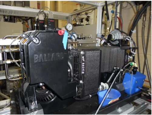
7. APPENDIX A: SHORT MANUAL FOR NEXATM TEST BENCH ... 171
7.1 Test bench fundamentals and set-up ... 172
8. APPENDIX B: ELECTROCHEMISTRY OF THE ELECTRODE, FUNDAMENTALS ON FARADAIC
IMPEDANCE.... ... 177
ACKNOWLEDGEMENTS
I would like to express my gratitude to my academic advisers of the University of Salerno (UNISA) Prof. Cesare Pianese and Dr. Marco Sorrentino for their constant and essential support during these years. Their great knowledge, competence and perseverance combined with dedication and passion represented and represent for me a reference point. A special thanks goes to Prof. Gianfranco Rizzo and Prof. Ivan Arsie for their help and availability.
I wish to address my special thanks to my academic advisers of the University of Franche-Comté (UFC) Prof. Daniel Hissel and Prof. Marie-Cécile Péra who gave me the opportunity to have a great experience at the Fuel Cell Laboratory (FCLAB). Their professional competence and guidance combined with their courtesy have made my doctoral studies not only a very instructive but also a more enjoyable experience. I am also very grateful to Prof. Fréderic Gustin, Dr. Mohamed Becherif and Dr. Samir Jemei for their kind support. I am sincerely and intensely grateful to my colleague Zhixue Zheng for her invaluable collaboration and to Mr. Xavier François and Mr. Fabien Harel for their kind assistance during the experimental activity. A special thanks goes to all the staff of FCLAB and UFC for their reception, collaboration and availability.
I would like to express my gratitude to Prof. Gianfranco Rizzo of University of Salerno for agreeing to chair my doctoral committee.
I wish to address my special thanks to Prof. Delphine Riu of University of Grenoble and Prof. Mohamed Machmoum, director of the IREENA-CRTT Laboratory, for agreeing to review my thesis.
I would like to acknowledge Prof. Massimo Guarnieri of University of Padova for agreeing to examine my works.
This work has been performed within the D-CODE project funded under Grant Agreement 256673 of the Fuel Cells and Hydrogen Joint Technology Initiative. A thanks goes to all the participants of the D-CODE Project, particularly to Dr. Philippe Moçoteguy, Dr. Angelo Esposito and Dr. Nadia Yousfi-Steiner of the European Institute For Energy Research (EIFER) for their kind collaboration and availability and for the data provided for my PhD Thesis. I am also very grateful to Prof. Giovanni Spagnuolo and Dr. Giovanni Petrone of the Departement of Industrial Engineering (DIIN) of the University of Salerno for their kind collaboration. A thanks goes to all the Dantherm people for their kind support. Moreover, I’m also very grateful to Bitron and Cirtem people for the collaboration shown within the project.
I would like to thanks Dr. Sebastian Wasterlain for its courtesy. Its PhD Thesis represented both a guideline and a valid support for the development of my experimental activities.
I would like to acknowledge the work of Fouquet et al. entitled “Model based PEM fuel cell state-of-health monitoring via ac impedance measurements” (Journal of Power Sources, 2006; 159(2):905-13). This paper represented for me a reference point to develop my PhD Thesis.
I would like to express my gratitude to the Doctoral School of the University of Salerno and to the Doctoral School of the University of Franche-Comté for the work carried to provide this great opportunity to students.
I’m truly grateful to my “roommates” (staff and PhD. students) of the Laboratory I5 of the Department of Industrial Engineering and of FCLAB for their kind collaboration and courtesy, particularly to Mr. Giampaolo Noschese for his technical support. Moreover a special thanks is due to all
my friends and in particular to Monica for supporting me in this last part of my doctorate.
My utmost gratitude goes to my parents for motivating and support me throughout my studies. I would never write this thesis without their love and if they did not teach me the value of education in the first place.
LIST OF FIGURES
Figure 1.1: Single PEM fuel cell scheme. ... 4
Figure 1.2: Qualitative polarization curve. ... 7
Figure 1.3: Model-based fault diagnosis scheme; adapted from Ding [19]. ... 16
Figure 1.4: Non-model based classification [18]. ... 20
Figure 1.5: General structure of non-model based diagnosis [18]. ... 20
Figure 2.1: EIS application in nominal operating conditions [62]. ... 29
Figure 2.2: Phase vectors analysis. (a) AC signals in time domain. (b) Phase vectors in a complex plane. Adapted from Wasterlain (2010) [7] . 32 Figure 2.3: Bode diagram: phase; data available in literature[17]. ... 33
Figure 2.4: Bode diagram: magnitude; data available in literature [17]. . 34
Figure 2.5: Typical equivalent cell impedance in Nyquist diagram; data available in literature[17]. ... 34
Figure 2.6: Solartron ModuLab ECS; image available on the net. [www.solartronanalytical.com/our-products/potentiostats/modulab.aspx] ... 40
Figure 2.7: Electrodes assembling schema, adapted from Wasterlain [7]: (a) two electrodes; (b) three electrodes; (c) four electrodes. ... 42
Figure 2.8: Standard Kelvin connection scheme [8]. ... 44
Figure 2.9: Partial cell connection schemes: a) anode; b) cathode. ... 45
Figure 2.10: Multi-electrodes connection scheme. ... 46
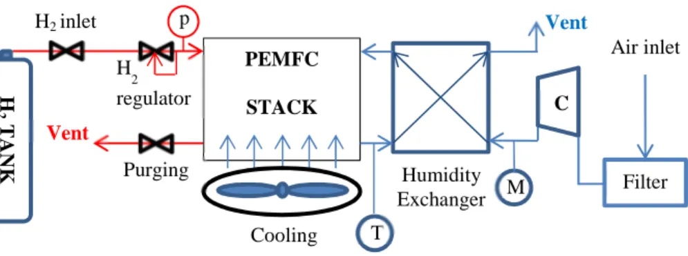
Figure 2.11: An example of ancillaries configuration for a test bench, adapted by Petrone et al. [8] ... 47
Figure 2.12: An example of test bench configuration for EIS. ... 49
Figure 2.13: An example of current closed loop generation in grounded measurements, adapted from Wasterlain [7]. ... 50
Figure 2.14: Commercial BALLARD NexaTM Power Module. ... 53 Figure 2.15: Qualitative NexaTM connection scheme: a) standard; b) EIS first configuration; c) ancillaries de-coupling [8]... 55 Figure 2.16: Ancillaries influence on NexaTM EIS measurements: i) for coupled ancillaries; ii) for de-coupled ancillaries configuration [8]. ... 57 Figure 2.17: Impedance spectra at normal operating condition performed on NexaTM [8]. ... 58 Figure 2.18: Impedance spectra at abnormal operating condition
performed on NexaTM [8]. ... 59 Figure 3.1: An example of EIS spectrum feature analysis for PEMFC equivalent cell: a) Nyquist diagram; b) semicircles analysis. Data
available in literature [17]. ... 66 Figure 3.2: Effects of current in impedance spectra and correlation with polarization curve. a) V-I curve; b) Impedance spectra at current
variation, particular of Ohmic resistance behaviour. c) Effect at low-medium current variation; d) Effect at low-medium-high current variation. Measurements referred to the NEXATM system [8]. ... 69 Figure 3.3: Effects of drying and flooding conditions (idc=466 mA/cm2): a) Polarization Curve; b) Nyquist diagram. Represented data has been adapted by Fouquet et al. [17]. ... 70 Figure 3.4: Effects of air stoichiometric factor variation in PEMFC, adopted by Petrone et al. [8] ... 72 Figure 3.5: Influence of CO poisoning, after Wagner et al. [71]. ... 73 Figure 3.6: An example of Randles’ model; ZF splitting for the simplest and mixed kinetics and diffusion configurations. ... 76 Figure 3.7: ECM behaviour: a) at high frequencies; b) at low frequencies. ... 77 Figure 3.8: Ohmic resistance representation in Nyquist plot. ... 78 Figure 3.9: Charge storage at CDL interface; a capacitive behaviour. .... 80 Figure 3.10: Qualitative Nyquist plot representation of the ideal
polarization of the electrode. ... 82 Figure 3.11: Qualitative representation of the Randles’ model on the Nyquist plot. ... 84
Figure 3.12: Qualitative representation of the effects of Warburg elements in the Faradaic impedance spectrum: the red line characterizes the
semi-infinite element, while the black arc characterizes the finite one. ... 87
Figure 3.13: Qualitative representation of the equivalent impedance spectrum in case of diffusion. ... 88
Figure 3.14: CPE modelled as a distributed capacitor for porous electrode characterization. Adapted by Fontés [92]. ... 89
Figure 3.15: CPE influence for ideal polarization of the electrode... 90
Figure 3.16: CPE application in Randles’s circuit (simple case: no diffusion); semi-circle rotation. ... 90
Figure 3.17: An example of dissociated electrodes models: a) complete model; b) simplified model. ... 92
Figure 3.18: Effects of cabling in Nyquist representation. ... 94
Figure 3.19: Relation between the polarization curve slope and the arcs deformation in the main dominant losses regions (a), (b) and (c). ... 96
Figure 4.1: Randles model configuration for mixed kinetics and diffusion losses adopted by Fouquet et al. [17], along with associated model parameters. ... 102
Figure 4.2: Convergence of NM method. ... 103
Figure 4.3: 2-norm residual values distribution for 1024 random identifications. ... 104
Figure 4.4: Impedance spectra extrapolated by the first 2-norm class; Ref. data were retrieved from Fouquet paper [17]. ... 104
Figure 4.5: Identifications in case of perturbed data: a) all the spectrum is perturbed (5.6% of deformation with respect to the reference shape); b) the spectrum is perturbed only at low frequencies (4.9% of deformation with respect to the reference shape). EIS data retrieved from Fouquet et al. [17]. ... 105
Figure 4.6: Influence of the Ohmic resistance variation. ... 107
Figure 4.7: Influence of the charge transfer resistance variation. ... 107
Figure 4.8: Influence of the CPE capacitance variation. ... 108
Figure 4.9: Influence of the CPE coefficient variation. ... 108
Figure 4.11: Influence of the Warburg time constant variation. ... 109
Figure 4.12: Off-line procedure usually adopted in ECM fitting. ... 114
Figure 4.13: Proposed identification procedure - Flow Chart. ... 115
Figure 4.14: Complete starting reference model assumed in GFG. ... 117
Figure 4.15: GFG simplified ECM configurations. ... 118
Figure 4.16: GFG evaluation of presence of the diffusion arc. ... 119
Figure 4.17: Charge transfer semi-circle characterization. ... 120
Figure 4.18: Geometrical evaluation of R and C. ... 121
Figure 4.19: GFG flow chart. ... 123
Figure 4.20: Results of the identifications for the Fouquet data [17] in flooding, normal and drying conditions. ... 127
Figure 4.21: Convergence of CNLS fit assisted with GFG. ... 129
Figure 4.22: Identification for data affected by noise. EIS data were retrieved from Fouquet et al. [17] ... 130
Figure 4.23: 2-norm distribution of the 1024 identification evaluated with respect to the EIS data. ... 131
Figure 4.24: NexaTM polarization curve and temperature distribution. .. 132
Figure 4.25: Fitted spectra for NexaTM system in case of current variation: a) fitted spectra; b) data matching from 5.33 to 21.9 A; c) data matching from 21.9 to 44.4 A. ... 133
Figure 4.26: Spectra fitted for NexaTM system at 20 A varying the air stoichiometric factor (Air St.). ... 135
Figure 4.27: Dantherm® DBX2000 polarization curve [100]. ... 136
Figure 4.28: Fitted spectra for Dantherm® DBX2000 module in normal operating conditions: a) fitted spectra at current variation; b) data matching from 4.30 to 25.52 A; c) data matching from 25.52 to 43.84 A. Data provided by EIFER [100]. ... 138
Figure 5.1: Dantherm® DBX2000 power backup module; picture available on the net: www.e-fbg.com/services/hidrogeno. ... 142
Figure 5.2: Open-cathode configuration. ... 143
Figure 5.3: Procedure for off-line parameter models development. βk is the identified parameters’ vector for the k-th measured operating conditions (M.O.C). ... 145
Figure 5.4: On-line diagnosis flow chart: part 1. Monitoring and
simulation. ... 146
Figure 5.5: On-line diagnosis flow chart: part 2. On-board identification and fault detection. ... 148
Figure 5.6: Negative maximum phase angle physical meaning in phase vector analysis. Data provided by EIFER [100]. ... 150
Figure 5.7: Equivalent Ohmic resistance representation... 152
Figure 5.8: Equivalent faradaic resistance representation... 155
Figure 5.9: CPE capacitance representation... 156
Figure 5.10: CPE coefficient representation. ... 157
Figure 5.11: Maximum negative phase angle representation... 158
Figure 5.12: Impedance spectra simulation for diagnosis; an example for normal, acceptable and abnormal conditions. ... 159
Figure 5.13: Analysis of identified parameters at about 10 A in different operating conditions. Starting drying out detection. ... 160
Figure 5.14: Initial flooding condition detection. ... 162
Figure 7.1: NexaTM test bench. ... 171
LIST OF TABLES
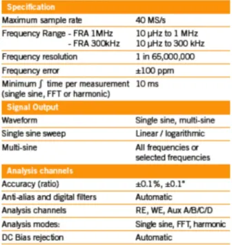
Table 1.1: Abnormal operating conditions due to external factors. ... 11 Table 1.2: Abnormal operating conditions: unexpected working variables variation... 14 Table 1.3: Model comparison for PEMFC applications [2]. ... 17 Table 1.4:List of acronyms for non-model based techniques. ... 19 Table 2.1: An example of FRA specification, adopted by Solartron
ModuLab brochure
[www.solartronanalytical.com/our-products/potentiostats/modulab.aspx]. ... 41 Table 3.1: EIS application for PEMFC characterization and degradation processes. ... 63 Table 3.2: EIS application for PEMFC diagnosis. ... 64 Table 4.1: Parameter significance for normal conditions. ... 110 Table 4.2: Parameter significance for flooding conditions. ... 111 Table 4.3: Parameter significance for drying conditions. ... 111 Table 4.4: Parameter correlation matrix in normal conditions. ... 112 Table 4.5: Parameter correlation matrix in flooding conditions. ... 112 Table 4.6: Parameter correlation matrix in drying conditions. ... 112 Table 4.7: Data sets exploited for the GFG algorithm validation. ... 125 Table 4.8: Identified parameters for data set A. ... 127 Table 4.9: Identified parameters presented by Fouquet [17]. ... 128 Table 4.10: Identified parameters for NexaTM system at current variation. ... 134 Table 4.11: Identified parameters for NexaTM system at 20A: tests
performed at different values of the air stoichiometric factor (Air St.). 135 Table 4.12: Dantherm® DBX2000 normal operating conditions [100]. 137 Table 4.13: Identified parameters for Dantherm® DBX2000 module in normal operating conditions. ... 139
Table 5.1: Fault to symptoms matrix (FSM). ... 145 Table 5.2: Qualitative parameter residual analysis. ... 162
NOMENCLATURE
Acronyms
AC Alternating Current
AFC Alkaline Fuel Cell
ANN Artificial Neural Network
ANFIS Adaptive Neuro-Fuzzy Inference Systems
BN Bayesian Network
BoP Balance-of-Plant
CDL Charge Double Layer
CE Counter Electrode
CNLS Complex Non-linear Least Squares
CPE Constant Phase Element
DC Direct Current
D-CODE DC/DC COnverter-based Diagnostics for PEM
systems
DoE Department of Energy
ECM Equivalent Circuit Model
ECSA Electrochemically Active Surface Area
EIFER European Institute For Energy Research
EIS Electrochemical Impedance Spectroscopy
EL Electric Load
FC Fuel Cell
FCLAB Fuel Cell Laboratory
FL Fuzzy Logic
FDA Fisher Discriminant Analysis
FDI Fault Detection and Isolation
FFT Fast Fourier Transform
FRA Frequency Response Analyser
FSM Fault to Symptom Matrix
GDL Gas Diffusion Layer
GFG Geometrical First Guess
HOR Hydrogen Oxidation Reaction
KFDA Kernel based Fisher Discriminant Analysis
KPCA Kernel based Principle Component Analysis
LM Levenberg-Marquardt
MCFC Molten Carbonate Fuel Cell
M.O.C. Measured Operating Conditions
MPL Micro-Porous Layer
NM Nelder-Mead
O.C. Operating Conditions
OCV Open Circuit Voltage
ORR Oxygen Reduction Reaction
Ox Oxidation
PAFC Phosphoric Acid Fuel Cell
PC Personal Computer
PCA Principle Component Analysis
PEMFC Proton Exchange Membrane Fuel Cell
PF Particle Filter Rd Reduction RE Reference Electrode Res Residuals RH Relative Humidity SA Simulated Annealing
SHE Standard Hydrogen Electrode
SOFC Solid Oxide Fuel Cell
SVM Support Vector Machines
STFT Short-Time Fourier Transform
WPE Working Power Electrode
WSE Working Sense Electrode
WT Wavelet Transform
Roman Symbol
C carbon
Cb bulk concentration (mol/m3)
Cdl double layer capacitance (F=s/Ω) – capacitor
CS surface concentration (mol/m3)
CO carbon monoxide
D diffusion coefficient (m2/s)
d distance between the plates of a capacitor (µm)
E cell potential (V)
E0 theoretical cell voltage (V)
Eeq equilibrium reaction potential (Nernst potential) (V)
e residual (-)
e- Electron
F Faraday constant (96485 C/mol)
f frequency (Hz)
f(xi) expected data
G Gibbs free energy (kJ/mol)
GR ground
H enthalpy - thermal energy (kJ/mol)
H2 hydrogen
H2O water
H+ hydrogen proton
I current (A)
i current density (A/cm2)
i0 exchange current density (A/cm2)
il limited current density (A/cm2)
j imaginary unit (-1)
L inductance (H=Ωs) – inductor
l electrolyte thickness (m)
Mcf membrane resistance correction factor (-)
n number of electrons participating to the reaction (-)
nc number of cells (-)
O2 Oxygen
Obj_F objective function
P pressure (Pa)
Pt platinum
Q CPE capacitance (sϕ/Ω)
R universal gas constant (8.314 J/mol/K)
R resistance (Ω)
Rd diffusion resistance (Ω)
RF Faradaic resistance (Ω)
Rp polarization resistance (Ω)
RΩ Ohmic resistance (Ω)
S entropy
SA active surface area (cm2)
sulfonated group T temperature (K) t time (s) V voltage (V) ||v|| vector 2-norm (-) w weight (-)
Wel maximum electric work (kJ/mol)
yi measured data
Z impedance (Ω)
|Z| impedance magnitude (Ω)
∠ impedance maximum negative phase angle (rad)
ZF Faradaic impedance (Ω)
ZW Warburg impedance (Ω)
Greek Symbols
α charge transfer coefficient (-)
β symmetry factor of the reaction (-)
βm parameters
βsign parameter significance (-)
∆ change of …
δ diffusion layer thickness (m)
ε efficiency (-)
εc electrical permittivity (F/m)
η overpotential (V)
ηact activation losses (V)
ηd diffusion losses (V)
ηΩ Ohmic losses (V)
θ phase displacement (rad)
λst stoichiometric factor (-)
µ chemical potential (V)
ϕ CPE coefficient (-)
φ impedance phase (rad)
σ mass transfer coefficient (m/s)
σE charge density of the electrode (C/m2)
σel electrolyte conductivity (S/cm)
σi standard deviation (-)
τ time constant (s)
τd Warburg time constant (s)
χ2 Chi-squared (-)
ω radial frequency (rad/s)
Subscripts act activation a anode b bulk c cathode cen centre cell cell d diffusion el electrolyte eq equivalent – specific F Faradaic
finite finite dimension
id identified l limited meas measured mod modelled O oxidant p polarization R reductant S surface s simulated
Sign significance th theoretical Var variation W Warburg Ω Ohmic 0 reference
SUMMARY
Proton Exchange Membrane, also named Polymer Electrolyte Membrane fuel cells (PEMFC) are interesting devices for energy conversion. Their development is due to the high efficiency, acceptable power density, quick start-up and good environmental compatibility [1-3]. On the other hand, reliability cost and durability are the main challenges for PEM fuel cell commercialization. In 2010 the American Department of Energy (DoE) sets a target of 40000 hours for stationary and 5000 hours for automotive applications, respectively [4,5]. Actually, these standards are considered as the mainly reference in fuel cell research.
Based on electro-catalytic reactions, the PEMFC operation is influenced by system functioning conditions. In case of system operation in abnormal conditions several chemical, mechanical and thermal degradation mechanisms could take place inside the cell. Among other, improper water, thermal and gas managements can introduce a cell voltage drop, thus reducing the system performance [3,4]. A long-term exposure to these phenomena causes the PEMFC lifetime reduction. Thus, a good system management is one of the primary targets to ensure suitable PEMFC durability. For this purpose, research activities are oriented towards the development of newest advanced monitoring and diagnostic algorithms. The primary goal is monitoring the system operation ensuring a correct system control. Moreover, the diagnostic tool (i.e. both algorithm and sensors) allows the detection of system component malfunctioning; it can isolate one or more faults that may have occurred causing the abnormal behaviour of the system operation.
In common commercial systems the operating variables, such as stack voltage, current and temperature are usually monitored for control purposes. The measured signals are then processed through a control board that provides the right control signals to the ancillary devices for the correct operation. However, usual control strategies are finalised to guarantee the system operation in acceptable conditions only, without taking into account any actions for performance recovery. In this contest, advanced research studies, both at experimental and theoretical levels, may support the development of effective monitoring and diagnostic algorithms. From these algorithms the control actions may also be improved by using the knowledge of the system actual status, which in turn can improve the performance. Therefore, the development of appropriate control strategies, as well as accurate fault detection algorithms, are required to attain a longer lifetime. In this scenario, the capability to identify in real-time the PEMFCs state-of-health and related degradation mechanisms is one of the main objectives.
This work aims at developing a parameter identification algorithm for on-board fault detection and isolation (FDI) applications based on the electrochemical impedance spectroscopy (EIS) technique. The EIS is a
non-invasive experimental technique [6], usually applied for
electrochemical system analysis. This procedure stimulates the main physical phenomena involved in PEMFC. Its use is based on the injection of a sinusoidal signal, which perturbs the system at known frequencies. Then, by analysing the system response it is possible to de-couple different electrochemical processes, isolating the PEMFC losses (i.e Ohmic, kinetic and mass transport) [7,8]. Therefore, the idea is to extrapolate and then exploit the information on PEMFC status, which cannot be directly achieved through the cell voltage drop monitoring. To exploit the information brought by EIS data, an equivalent circuit model (ECM) is considered. This allows accounting for the different electrochemical phenomena occurring inside the cell. In each electrical component of the model one or more parameters can be identified.
Through their trends it is possible to monitor the system behaviour, and then, to check the possible fault when the system runs.
This work faces two problems: the on-board implementation of EIS and the on-line model parameter identification. The first topic is related to the measurement reliability, which is influenced by system internal and external factors. On the other hand, the second one is oriented to solve the multi-minima problems involved in the minimization function, which can severely compromise the results of the identification process. Moreover, the work aims at replacing the human experience with a carefully automated strategy for the data analysis implementation. Indeed, in common EIS applications, the expertise of the operator is always required for the data interpretation. The proposed procedure performs the automated selection of both the ECM configuration and proper starting parameters values for the fit.
The interpretation of the identified parameters is made through some regression models, which link the parameter changes to the operating conditions variability. For system monitoring, an ECM simulates the impedance spectrum by using the parameters derived from the regressions evaluated at normal operating conditions. Then, the simulated impedance spectrum and the measured one are compared for evaluating residuals. If residuals are less than a fixed threshold, the system operates in normal conditions, otherwise the on-line parameter identification procedure starts. The fault detection and isolation are performed by comparing the values of the identified parameters with their trends expected for the actual operating conditions. Then, it is possible to detect the occurrence of faults when one or more residuals are above the fixed thresholds. For this purpose, a fault to symptoms matrix for drying out, flooding and air starvation is proposed.
This work has been performed within the D-CODE project (website: https://dcode.eifer.uni-karlsruhe.de) funded under Grant Agreement 256673 of the Fuel Cells and Hydrogen Joint Technology Initiative. Its
aim is to develop a diagnostic tool for on-line monitoring and FDI based on EIS. For this purpose the classical EIS single-frequency approach based on small amplitude signal injection has been considered. In the context of the project D-CODE, this thesis deals with two relevant issues: the measurements reliability and the impedance spectra analysis.
1.
INTRODUCTION
Nowadays, hydrogen is playing an increasing role in the area of the “green” energy conversion. Therefore, Fuel Cells (FCs) are considered a promising solution due to their high efficiency, acceptable power density and good environmental compatibility [1-3]. Particularly, Proton Exchange Membrane, also named Polymer Electrolyte Membrane fuel cells (PEMFC) have gained a relevant position in both stationary and transportation-oriented applications, such as power backup systems, portable devices, educational kits, automotive and boat propulsion.
Reliability, cost and durability are the main challenges for PEMFC commercialization. Many researches have been carried out in order to develop new materials and advanced management of these systems. Indeed, one of the main aspects is the system durability. In order to improve the PEMFC lifetime, in 2010 the American Department of Energy (DoE) sets a target of 40000 hours for stationary and 5000 hours for automotive applications, respectively [4,5]. These standards are considered as the mainly reference in fuel cell research. Based on the electro-catalytic reactions, the PEMFC operation depends on several physical phenomena occurring inside the cells. The system operation in abnormal conditions, such as improper water management, catalyst degradation and fuel starvation [3,4] may introduce a performance drop and even reduce the lifetime of a PEMFC. Thus, a good system management is one of the primary targets to ensure suitable PEMFC durability. To this purpose, the development of advanced monitoring system and diagnosis algorithms appears as an important milestone in PEMFC research.
In this chapter the main generalities of PEMFC operation are introduced, by analysing the effects of both the normal and abnormal operating conditions. Moreover, a comprehensive review of PEMFC diagnosis approaches, which are available in the literature, is detailed. This part summarises the initial state-of-art analysis and represents the bases to introduce the research activities. Consequently, the objective and the expected contribution of this research are depicted.
1.1
Generalities on PEMFC systems
Fuel Cells are interesting devices for energy conversion based on the electro-catalytic reactions. Generally these systems are composed of different cells connected in series, of which the assembling is also named stack. During PEM operation, the electrochemical reactions occur in each cell, satisfying the current demand; the stack voltage is achieved considering the sum of the potential related to the single cell electrodes. In literature several types of fuel cells are available, which are classified according to their electrolytes: alkaline fuel cells (AFC), molten carbonate fuel cells (MCFC), phosphoric acid fuel cells (PAFC), polymer electrolyte membrane or proton exchange membrane fuel cells (PEMFC) and solid oxide fuel cells (SOFC) [9-11]. This work focuses on PEMFC systems, whose name derives from the polymer membrane, which allows the H+ protons’ exchange. One of the advantages to adopt a solid polymer electrolyte is the reduction of both the corrosion phenomena and the gas cross-over. Moreover, operating at low temperatures, less than 80 °C, the PEMFC design is very simple, if compared with the other systems, and allows a rapid start-up. Nevertheless, concerning the possibility of CO poisoning, the use of quite pure hydrogen is required. To understand the PEMFC operation, the electrochemical reactions involved in a single H2/air PEM cell are reported below:
: → 2 + 2 (Eq. 1.1)
: + 4 + 4 → 2 (Eq. 1.2)
The reaction 1.1 and 1.2 are referred to the hydrogen oxidation reaction (HOR), at the anode side, and to the oxygen reduction reaction (ORR), at the cathode side, respectively. Thus, the global reaction is:
+ 2 → 2 (Eq. 1.3)
Moreover, due to the system operation at low temperature, a catalyst, such as platinum (Pt), is usually employed to support the reaction kinetics. The single cell functioning is drafted in figure 1.1. The reactants, fuel at the anode and air at the cathode, are directly fed from the bipolar plate flow channels to the porous electrodes. Concerning the carbon electrodes, it is possible to distinguish two main layers, one dedicated to the gas diffusion and the other one aimed at the electrochemical reaction activation, also named catalyst layer. Due to its hydrophobicity, the diffusion layer is optimized in such a way as to ensure the water removal, which in turn allows the correct gas feeding to the activation area. It is possible to distinguish two sub-layers, a big one named GDL (about 125 - 350 µm) and a small one named micro-porous layer (MPL) (about 25 – 35 µm) [12]. The hydrophobic coating also shields the layer structure from the corrosion. Indeed, though the carbon fibres of the GDL result quite stable, they are still exposed to the produced water and to the convective reactant flow [12,13]. On the other hand, the catalyst layer is mainly aimed at increasing the activation of the electrochemical reactions (i.e. eq. 1.1 and 1.2). This layer is composed by the same carbon black particles of the MPL, loaded with nano-scale particles of Pt and mixed with the ionomer [12]. Moreover, the carbon supports of the electrodes facilitate the electron conductivity and the heat transport. The electrochemical reactions occur at the interface catalyst layer/electrolyte, where reactants, catalyst and electrons are available; this area is also named electrochemically active surface area (ECSA). In case of fuel impurities,
such as the carbon monoxide (CO), the catalyst poisoning is induced blocking the catalytic sites and then reducing the ECSA [11]. Thus, to prevent the carbon oxidation and the Pt dissolution and agglomeration phenomena, the use of quite pure hydrogen is strictly required. A proton exchange membrane, usually composed of perfluorosulfonated polymer (Nafion®), allows the charge transfer from the anode to the cathode side in a hydrated form [11].
Figure 1.1: Single PEM fuel cell scheme.
Air H2O Cooling (1) (2) (3) (4) (5) 150-350 µm 25-35 µm 10 µm F | C | F F | C | F F | C | F F | C | F F | C | F F | C | O | C | C | O | C | C | S | O F | C | F F | C | F F | C | F F | C | F F | C | F – – – – – – – – – – – – – F – – F F – – F F – – F F – – F O = = O (– ) H (+) H O H (1) Bipolar plate (2) GDL (3) MPL (4) Catalyst layer (5) Electrolyte H2 2H2 H2O 4H+ Vent Air H2O O2 4e -Anode Cathode Electrolyte i Vent Heat 4e -(C) (C) Heat G D L G D L Electrode (Pt) (Pt) Electrode (1) (2) (3)(4) (5)
Then, the proton conductivity is strictly related to the membrane water content. Two main water flows can be seen: the electro-osmotic drag and the back-diffusion. The first one characterizes the water brought by the proton transfer from the anode to the cathode, while the second one is related to the water gradient between the cathode and anode sides. Indeed, the superimposition of the electro-osmotic drag and of the ORR water generation leads to an increase of the water content at the cathode side; conversely the high water content causes the back diffusion of the water towards the anode side. If not balanced, these flows can reduce the system performance, inducing either the anode drying out or the cathode flooding [3,11]. Moreover, the Nafion® properties depend on the system temperature, which must never overcome 80°C. To ensure the system operation, several ancillaries are required for the reactant feeding, the water management, the electrical production management and the system cooling. All these components are also named balance-of-plant (BoP). This point will be clarified in section 2.3.1 (figure 2.11).
1.2
Fundamentals of PEMFC analysis
The PEMFC structure has been introduced in the last paragraph. According with the aims of this work the fundamentals of the PEMFC analysis are then presented. The maximum electric work achievable by a fuel cell is expressed by the Gibbs free energy through the relationship reported below:
= ∆ = −!"#$ (Eq. 1.4)
Where n is the number of the electrons involved in the reaction (for eq. 1.1 ! = 2), while F 96487 )* +,-⁄ / is the Faraday constant. #$ is the theoretical cell voltage assumed as the difference between the anode and cathode potentials. In case of standard conditions at 25 [°C] and 1 [atm],
for liquid water production, ∆ = −237 )12/+,-/, while in case of water vapour production ∆ = −229 )12/+,-/. Thus, in standard conditions the thermodynamic cell voltage #$ is 1.23 [V] and 1.19 [V] for liquid water and vapour production, respectively [11]. According to the Nernst equation, it is possible to compute the equilibrium potential related to the gas properties as follows:
# 4 = #5− #6 = #$+789-! :;<=
> =⁄ ; ?=
;?=< @ (Eq. 1.5)
where in case of liquid water production AB=C is assumed equal to 1. In real world applications, the open circuit voltage (OCV) is assumed as the maximum cell voltage achievable when no load is applied (the cell current is 0). Its value is always lower than 1.23 V, due to the Pt oxidation and H2 crossover from the anode to the cathode side [11]. Moreover, when a load is applied, the cell voltage decreases.
The theoretical efficiency can be estimated as the ratio between the Gibbs free energy and the thermal energy (enthalpy change) available for the H2/air cell reaction ∆ = 285.8 )12/+,-/ in standard conditions. Thus, at 25°C the efficiency is:
FGH =∆I∆B≈ 0.83 (Eq. 1.6)
By replacing the Gibbs free energy by its thermodynamic equation:
FGH =∆I∆B= 1 −8∆M∆B (Eq. 1.7)
it is possible to remark that efficiency decrease with increasing temperature depending on the entropy change ∆ of the reactions [11].
Usually, the cell voltage variation with respect to the current (or to the current density1) is represented through the V-I curve also named polarization curve, reported in figure 1.2. Then, a first way to assess the system operations is to evaluate the cell voltage drop. Indeed, the voltage reduction is characterized through the superimposition of three fundamental losses: i) the activation, ii) the Ohmic and iii) the mass transport.
Figure 1.2: Qualitative polarization curve.
The trend of the losses related to the reaction kinetics, also named activation losses, is represented in figure 1.2 with the red curve. These
1 The current density is the ratio between the operating current and the active surface area of the cell.
0 200 400 600 800 1000 0 0.2 0.4 0.6 0.8 1 1.2 Polarization Curve i [mAcm-2] V c e ll [ V ] E0 OCV Activation Losses Ohmic Losses
Mass Transport Losses V-i Curve
losses characterize the activation overpotential2 irreversibility of the reactions both at anode and cathode side. When a load is applied to the cell, the operating current passes through the electrodes changing their potential and, then, inducing a performance loss [11]. Moreover, as shown in figure 1.2, the voltage drop contribution due to the reaction kinetics is dominant at low current densities, where the charge transfer is the most important irreversibility. The activation losses involve both the electrodes, though their contribution is more significant at the cathode side [10]. Based on Tafel’s law, the activation losses are related to the current density through the following equation:
N65G=OP978 -! QRRST (Eq. 1.8)
Where R and F are the universal gas constant and the Faraday constant, respectively, n is the number of electrons involved in the reaction and T is the temperature in Kelvin. The constant U is the charge transport coefficient, while V$ is the exchange current density [9-11].
The Ohmic losses are represented in figure 1.2 with the blue line. Their voltage drop contribution is strictly proportional to the current density and is more significant in the mid-point of the polarization curve; the related equation is:
NW= W, 4∙ V (Eq. 1.9)
Where W, 4 is the specific (or equivalent) resistance expressed in )Z[+ /, which involves all the internal resistances of the cell, such as both the electrodes and the electric contact resistances to the electron flow and the electrolyte proton resistance. Among these, the membrane resistance is the most significant one [10,11].
2 The difference between the applied potential and the electrode equilibrium potential (or Nernst potential) is defined overpotential (E-Eeq).
The losses due to the mass transport phenomena are represented in the figure 1.2 with the green curve. In order to supply the reactions, the reactants need to reach the catalyst layer. Then, the slow electro-active species transport to the reaction site induces a loss of the electrode potential. This loss is due to the inability of the reactants flow to maintain the bulk concentration at the electrode/electrolyte interface. Several causes can contribute to the mass transport voltage drop, among these the gas starvation and the slow diffusion in the GDL pores are the most significant ones [9]. As reported in figure 1.2, the diffusion losses are mostly significant at high current densities. The rate of the mass transport to the electrode surface is expressed through the Fick’s first law of diffusion [9], in which the value of the resulting current density can be computed as a function of the gradient of the concentrations:
V =P9\ ]^ ]_
` (Eq. 1.10)
where D is the diffusion coefficient and a is the diffusion layer thickness, while *b and *c are the bulk concentration and the surface concentration, respectively. The maximum rate at which a specie can be supplied on the electrode surface is then achieved imposing *c = 0 ; this condition is also named limited current density V [9]. The mass transport losses are related to the current density as follows:
Nd =78P9e-! Q1 −RRfTe (Eq. 1.11)
Therefore considering the afore introduced relationships, the global cell voltage drop under normal operating conditions can be evaluated as [9-11]:
g5 = #4− N65G− NW− Nd (Eq. 1.12)
It is worth remarking that analysing the polarization curve it is possible to evaluate the global voltage drop, but the single contribution of the different losses is difficult to distinguish. Then to separate the
different irreversibilities, other methods are commonly employed in PEMFC analysis, such as the current interruption, the cyclic voltammetry, the chronoamperometry and the electrochemical impedance spectroscopy. This work focuses on the electrochemical impedance spectroscopy, which will be introduced in the next chapter; for the other techniques more details can be found in the literature [10,11,14].
1.3
PEMFC operation in abnormal conditions
In the last paragraph the main irreversibilities of the PEMFC in normal operating conditions have been introduced. Nevertheless during the system operations several factors can influence the PEMFC status. Indeed, a variation of the working variables automatically induces a change of the system equilibrium state. The causes of abnormal operating conditions can be related both to the occurrence of external factors and to the unexpected variations of the system working variables [13]. Among others, the presence of impurities in fuel/oxidant gas and ambient cold temperature (subfreezing conditions) are considered as the most relevant external agents. Instead, potential cycling, fuel starvation, start/stop cycling and improper stack temperature and water management are related to unexpected changes in working in operating conditions.
An overview on the effects of abnormal conditions is reported in the following, for more details the reader is addressed to the scientific literature [12,13,15,16]. In case of fuel and oxidant impurities, the overpotential losses raise due to the impurities adsorption at the anode and at the cathode catalyst layers, respectively. Moreover, their presence does not affect only the charge transfer mechanisms; indeed, the dissolved parts can also induce the membrane poisoning and affect both water and gas transport behaviour [13]. The kind of the impurity and the period of
the components exposure determine whether the process is reversible or not. When the system starts at subfreezing conditions, the low reaction kinetics induces the main voltage loss. Nevertheless, the ice formation also results in Ohmic and mass transport voltage drops [13,16]. Although the limited cycling in subfreezing conditions are not so influent in terms of PEMFC durability, a long exposure to ice can generate several mechanical stresses, which in turn may irreversibly damage the system [13]. The effects of the abnormal operating condition related to the external factors are resumed in Table 1.1.
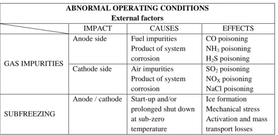
Table 1.1: Abnormal operating conditions due to external factors. ABNORMAL OPERATING CONDITIONS
External factors
IMPACT CAUSES EFFECTS
GAS IMPURITIES
Anode side Fuel impurities Product of system corrosion
CO poisoning NH3 poisoning H2S poisoning Cathode side Air impurities
Product of system corrosion SO2 poisoning NOX poisoning NaCl poisoning SUBFREEZING
Anode / cathode Start-up and/or prolonged shut down at sub-zero
temperature
Ice formation Mechanical stress Activation and mass transport losses
Concerning the system working variables, PEMFCs are designed to operate at different loads and, thus, no strong effects are observed in steady state operating conditions. However, rapid changes in load, high voltage conditions and improper start-up/shut down cycling can seriously compromise the PEMFC durability. Indeed, these abnormal operations change the cathode potential affecting the oxide coverage of both the platinum and carbon [13]. Then, the Pt dissolution and re-deposition and
the carbon corrosion take place reducing the Electrochemically Active Surface Area (ECSA) [12,13]. Moreover, the Pt dissolution at high voltage operation can also induce effects in the membrane, allowing the formation of the hydrogen cross-over mechanism [12], while a long exposure to the carbon corrosion could seriously affect the carbon surface hydrophobicity and then the GDL gas permeability [12]. In case of system operations in sub-stoichiometric conditions, a deep voltage drop is detected. Several factors cause the gas starvation, among the others flooding conditions and ice formation in GDL could block the reactant feed towards the ECSA. Therefore, the reactant starvation causes the cell voltage drop, first of all due to the mass transport phenomena, and then due to the permanent electrochemically activation area losses. The main effect of the reactant starvation is the reverse potential condition. In this case the cell potential is negative, inducing the carbon oxidation into the anode catalyst layer [13,15]. In particular, a fuel starvation causes the anode potential to raise, while the oxygen starvation induces the cathode potential reduction. Apart from the sub-stoichiometric conditions, the high temperature, combined with an improper water management, can also reduce the cell performance. Indeed, this condition causes the membrane dehydration, thus reducing the electrolyte proton conductivity, especially at the anode side. Moreover, if the membrane operates for a long period in dried conditions, the presence of hot spots can induce the formation of pinholes [15]. Furthermore, the increment of the activation losses is also observed in case of system drying out. Then, if the system runs in dried conditions for a short period, the performance losses are reversible. On the contrary, if the system operates for a long time, the degradation process occurs. Indeed, a long exposure to dried conditions induces the carbon corrosion and the Pt dissolution and agglomeration processes [13,15]. Opposite to dry out, an improper water management can also produce an accumulation of water both at the cathode and at the anode sides. This phenomenon is well known as flooding and occurs more frequently at the cathode side. As above mentioned, the presence of water in the GDL mainly affects the reactant transport to the catalyst sites.
Then, a cell voltage drop related to the mass transport phenomena is observed. Moreover, also an increment of the activation losses can be seen, as reported by Fouquet [17]. This effect might be due to a blockage of a part of the ECSA. As for the dry out, a short exposure to flooding conditions causes reversible losses, whereas a long exposure accelerates the electrode corrosion [15]. Moreover, if the exposure period is long, the dissolved catalyst can affect the membrane performance, by reducing the proton conductivity [15]. This process is mainly due to H+ ions replacement within the ionomer with impurities and corroded or dissolved parts. The main effects of PEMFC operations in abnormal conditions just introduced are summarized in Table 1.2.
As introduced in the last paragraph, the PEMFC operation automatically induces performance irreversibility. Nevertheless, in normal operating conditions the resulting voltage drop is acceptable. On the contrary, when an abnormal condition occurs, the performance losses raise up. If the exposure period to the undesired operations is quite short, the induced voltage drop should be reversible, otherwise the system degradation occurs. In order to guarantee the safe PEMFC operation, different diagnosis procedure have to be developed [2,18]. Indeed, these algorithms allow the system state-of-health monitoring, detecting the undesired operating conditions and the system faults when they occur. The diagnosis procedures are usually assisted by a controller, which tries to restore the system normal operations in case of unexpected working variable variation. In the next paragraph the generalities on PEMFC diagnosis are introduced. Specifically, in this work, an approach for on-line diagnosis is presented; particularly, in the last chapter the capability of detecting both drying out and flooding conditions is evaluated for a commercial system.
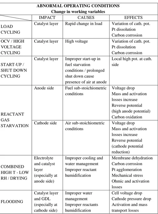
Table 1.2: Abnormal operating conditions: unexpected working variables variation. ABNORMAL OPERATING CONDITIONS
Change in working variables
IMPACT CAUSES EFFECTS
LOAD CYCLING
Catalyst layer Rapid change in load Variation of cath. pot. Pt dissolution Carbon corrosion OCV / HIGH
VOLTAGE CYCLING
Catalyst layer High voltage Variation of cath. pot. Pt dissolution Carbon corrosion START-UP /
SHUT DOWN CYCLING
Catalyst layer Improper start-up in fuel starvation conditions / prolonged shut down cause presence of air at anode
Local high pot. at cath. side
REACTANT GAS
STARVATION
Anode side Fuel sub-stoichiometric conditions
Voltage drop Mass and activation losses increase Reverse potential (high anode potential) Carbon oxidation Cathode side Air sub-stoichiometric
conditions
Voltage drop Mass and activation losses increase Reverse potential (cathode potential reduction) COMBINED HIGH T - LOW RH / DRYING Electrolyte and catalyst layer (especially at anode side)
Improper cooling and water management Improper reactant humidification Membrane dehydration Carbon corrosion Pt agglomeration Mechanical stress Ohmic and activation losses FLOODING Catalyst layer and GDL (especially at cathode side) Improper water management Improper reactants humidification
Cell voltage drop Cathode pressure drop Activation and mass transport losses
1.4
Generalities on diagnosis techniques for PEMFCs
As introduced before, the electro-catalytic reactions, which control the PEMFC operations, are influenced by several physical phenomena occurring inside the cells. Then, improper operating conditions may introduce system faults and degradation. These critical behaviours force the research activities to develop new monitoring and diagnosis techniques [2,18]. Indeed, the aim of these works is to ensure a good system management in order to improve the PEMFC performance and durability. The present work is aimed at developing a parameter identification algorithm for an innovative diagnostic tool based on electrochemical impedance spectroscopy (EIS). In order to contextualize the research objectives, an overview of different methodologies available in the literature for on-line PEMFC monitoring and fault detection and isolation (FDI) is reported in the following.
A suitable diagnostic tool aims at identifying in real time the faults that may occur in the system. Then, three main tasks can be found: the fault detection, fault isolation and fault magnitude analysis [2,18-21]. According to whether a model is needed, two main approaches can be considered: model-based and non-model based. For the former one, a suitable model simulates the system behaviour. In this case the diagnosis is performed by evaluating the residuals between experimental results and model outputs. Then, an inference analysis is done on the residuals to detect the possible fault occurrence [19,22]. An example of residual-based diagnosis is reported in figure 1.3. On the other hand, the non-model based methodologies focus on heuristic knowledge and signal processing or on a combination of them [2,18], thus no residuals are evaluated.
Concerning the model-based approach, a deep understanding of the real system is required to simulate the involved physical phenomena through mathematical laws. Usually, the models are classified depending
on the required physical knowledge in: white-box, grey-box and black-box.
Figure 1.3: Model-based fault diagnosis scheme; adapted from Ding [19].
White-box models, which are totally focused on physical knowledge, are usually exploited in PEMFC applications to model the electro-chemical, thermal and fluid-dynamic phenomena. Thus, the theoretical Nernst-Planck, Butler-Volmer and Fick’s laws are employed to characterize both the charge transfer and the mass transport phenomena. Nevertheless, although the white-box models are very accurate and show a high genericity, they require the solution of complex partial-differential equations and are not suited for on-line applications [2]. Moreover, these models involve several internal parameters that not always are easy to evaluate. In general, for on-line diagnosis grey and black-box models are implemented. On the other hand, the black-box models are developed via data-driven approaches and then they do not require the solution of physical models, allowing the achievement of faster algorithms. Moreover, these models ensure a high approximation of the non-linear phenomena. Nevertheless, they are strictly related to the training datasets, which must include all the system operating conditions, also the abnormal ones. Thus, the grey-box models have been considered to suitably
Process Process Model Input Output RESIDUAL GENERATION RESIDUAL EVALUATION Residual Processing Decision Logic
MODEL-BASED FAULT DIAGNOSIS
combine the physical knowledge and the data-driven advantages, replacing the complex differential equations with empirical formula or artificial intelligence structures. Then, the semi-physical models reduce the problem complexity allowing a good accuracy and genericity, also for non-linear phenomena. The comparison of model-based approach for PEMFC applications is summarized in Table 1.3.
Table 1.3: Model comparison for PEMFC applications [2].
White-box Grey-box Black-box
Structure complexity High Moderate Low
Accuracy High Good Good
Genericity High Good/Moderate Moderate/Low
Processing time High Moderate/Low Low
Physical knowledge High Moderate Low
Data-driven Low Moderate High
Application area System
understanding Off-line diagnosis
Training simulators
On-line FDI On-line FDI Control
Static models OK OK OK
Dynamic models OK OK OK
Non-linear response Good Good High
On-line applications Not indicated OK OK
In literature, the grey-box models used for PEMFC on-line FDI are usually organised in parameters-identification-based, observed-based, and parity space methods [19]. In parameter identification methods the model parameters are usually related to the physical phenomena. In this approach the parameters are estimated on-line and when the variation from their nominal values (i.e. in no faulty condition) achieves a certain threshold, the correlated fault is detected.
In general, the PEMFC monitoring is based on the analysis of the system electrical behaviour. The most common approach to reproduce the system working variables is the modelling of the electro-chemical phenomena through circuit-based models. Relevant results are available in literature in case of flooding detection [6,17,23,24]. Among others, the parameter identification methods based on EIS monitoring [17,24,25] appears the most suitable. Indeed, the EIS allows the association of each physical phenomenon to a specific equivalent circuit component; this point, which is the earth of this thesis, will be clarified in the next chapters. In particular the paper of Narjis et al. [24] can be assumed as the base ground for the development of on-board FDI based on EIS technique [2]. In observer-based [26,27] and parity space methods [28-30] the complex physical problems are usually reduced and linearized, by employing an observer or a parity space linear domain for residual calculation. The application of these methods to complex PEMFC models generates many residuals and only a certain number of them can be exploited for diagnosis. Therefore, these approaches are still under development, but are believed to be promising in future. A relevant contribution to PEMFC FDI development is also given by black-box models. The main feature of this approach is that the model parameters are not characterized by a physical meaning. Moreover they are evaluated through the interpolation of the training dataset rather than identification methods. Among others, artificial intelligence and heuristic techniques are often employed. Artificial neural networks (ANN) are usually used in non-linear dynamic modelling [31-35]; in such a method the training process needs a large amount of data. Therefore some authors [36-38] introduce also the application of fuzzy logic (FL) techniques for on-line PEMFC monitoring, especially in flooding detection. This methodology is very promising, but the on-line adjustment in case of new faults, which have not be considered a priori into the fuzzy rules, is difficult to achieve [2]. In order to solve this constraint the adaptive neuro-fuzzy inference systems (ANFIS) also have been developed [39-41]. Indeed in this method, the fuzzy rules are defined through the ANN approach, rather
than the a priori knowledge. Moreover the support vector machines (SVM) based on statistical learning are also tested in PEMFC diagnosis [42-44]. In general it can be stated that the black-box models show appreciable results for off-line applications, and that the on-line exploitations are still under development [2].
As mentioned above, non-model based approaches are also available in literature. These methodologies can be either knowledge-based or signal-based [18]. A detailed classification of the non-model based method is shown in figure 1.4. The main difference with the model-based approach is that the FDI is directly performed through fault classification procedures, without the use of residual inferences. Then, the experimental datasets are directly processed and normalized to extract the different features, which are relevant for fault classification [2,18]. Figure 1.5 resumes the most common steps involved in PEMFC non-model based diagnosis. The role of the related techniques is also reported. To simplify the dissertation the acronyms related to the non-model based approach are reported in table 1.4.
Table 1.4:List of acronyms for non-model based techniques.
ANFIS Adaptive Neuro-Fuzzy
Inference Systems KPCA Kernel PCA
ANN Artificial Neural Network KFDA Kernel FDA
BN Bayesian Network NN Neural Network
FDA Fisher Discriminant Analysis PCA Principle Component Analysis
FFT Fast Fourier Transform STFT Short-Time Fourier Transform
Figure 1.4: Non-model based classification [18].
Figure 1.5: General structure of non-model based diagnosis [18].
According to figure 1.4, three main non-model based methodologies can be outlined. In particular, artificial intelligence methods seem to be the most suitable ones for fault classification if discriminating features are considered [18]. Then, ANN, FL and ANFIS methods [45-48] are commonly employed for clustering technique application. At the same time, a second class of methods based on probability theory allows an
Non-model based approach Artificial Intelligence Statistical methods Signal processing methods
![Figure 2.5: Typical equivalent cell impedance in Nyquist diagram; data available in literature[17]](https://thumb-eu.123doks.com/thumbv2/123dokorg/5732362.74826/68.892.283.728.643.910/figure-typical-equivalent-impedance-nyquist-diagram-available-literature.webp)
![Figure 2.13: An example of current closed loop generation in grounded measurements, adapted from Wasterlain [7].](https://thumb-eu.123doks.com/thumbv2/123dokorg/5732362.74826/84.892.325.737.601.829/figure-example-current-generation-grounded-measurements-adapted-wasterlain.webp)
![Figure 2.15: Qualitative Nexa TM connection scheme: a) standard; b) EIS first configuration; c) ancillaries de-coupling [8].](https://thumb-eu.123doks.com/thumbv2/123dokorg/5732362.74826/89.892.204.503.243.721/figure-qualitative-connection-scheme-standard-configuration-ancillaries-coupling.webp)
![Figure 2.16: Ancillaries influence on Nexa TM EIS measurements: i) for coupled ancillaries; ii) for de-coupled ancillaries configuration [8]](https://thumb-eu.123doks.com/thumbv2/123dokorg/5732362.74826/91.892.117.587.252.684/figure-ancillaries-influence-measurements-coupled-ancillaries-ancillaries-configuration.webp)

