ELDERLY MORTALITY IN ITALIAN REGIONS AT THE BEGINNING OF THE HEALTH TRANSITION (1881-1921) L. Del Panta, D.G. Calò, L.M.B. Belotti
1. INTRODUCTION
In this paper we carry out an analysis of the territorial variation of elderly mor-tality (70–90 years) in Italy during the first stages of the health transition (between the end of the nineteenth and the beginning of the twentieth century).
The period in question includes forty years starting from the census of 1881 till the census of 1921; the territorial detail is that of regions (16 during the period). During this time frame the available data allow us to analyze mortality in four dis-tinct periods, namely in 1881-82, in 1900-01, in 1911-12 and in 1921-22.
It is a well-known fact that, at the beginning of the demographic transition, the main contribution to the increase of life expectancy at birth was given by the de-crease of infant, youth and – with a certain delay – adult mortality, while elderly mortality did not vary in a substantial way for a long time on, and in the very first stages of the transition seems actually to have increased. The life tables available at the moment for the overall Italian population1 show, in fact, a remarkable
in-crease of elderly mortality between 1881 and 1901.
We have therefore tried to check – also by analyzing the regional trends – the hypothesis that at least a share of that increase of the mortality risks could be fic-titious, that is, linked to the strong distortion of the age distribution of the popu-lation and of the deaths that characterizes the data of 1881. In fact, the distortion could cause an underestimation (Coale and Kisker, 1986; Thatcher, 1992; Preston et al., 1999) of the mortality risks in very advanced age.
We therefore took particular care in the construction of regional life tables based on 1881 census, in order to remedy, as far as possible, the inaccuracy of the data.
The chief aim of the paper was, however, to highlight and to analyze any pos-sible regional pattern of mortality at advanced age in the period of forty years (1881-1921) under consideration.
The paper is structured as follows. The second section deals with the trend of elderly mortality at national level in the forty years analyzed and stresses the
expected increase of mortality between 1881 and 1901. The third section is de-voted to problems linked with the construction of the life tables and of data reli-ability, especially regarding the 1881-82 tables. The fourth section provides a first look at the overall survival level of people aged 70 and over, in Italy on the whole as well as in the Italian regions, and briefly analyzes the cause mortality structure of the elderly at the beginning of the health transition. The fifth section presents the results of a multiway analysis (Bove and Di Ciaccio, 1994) carried out on the available data according to the STATIS method (Lavit et al., 1994); the aim of the study is to highlight regional differences in elderly mortality during the forty years period under investigation.
2. OLD AGE AND VERY OLD AGE AT THE END OF THE NINETEENTH CENTURY
Data in Table 1 show, both for male and female Italian population, the varia-tion – in the forty years under consideravaria-tion (1881-1921) – in overall survival and in mortality and survival at advanced age, and also allow a comparison with re-cent years (2006)2.
TABLE 1
Elderly survival and mortality in Italy, 1881-2006
m f 1881-82 1921-22 2006 1881-82 1921-22 2006 e0 35.24 49.24 78.44 35.76 50.72 83.98 l70/l0 0.2055 0.3638 0.7975 0.2104 0.3931 0.8927 l80/l0 0.0697 0.1308 0.5481 0.0656 0.1424 0.7330 l90/l0 0.0073 0.0089 0.1769 0.0061 0.0118 0.3441 20q70 0.9646 0.9756 0.7781 0.9711 0.9700 0.6145 e70 8.20 8.38 14.04 7.80 8.48 17.32 ex= 10 65.84 67.07 76.18 65.23 67.30 79.72
It is well known that the considerable increase in overall survival between 1881 and 1921 (about 15 years of life in males as well as females) was mainly caused by the sharp reduction of infant and child mortality (Caselli 1990, 1991, 2007; Pozzi 2000; Del Panta 1990). Nevertheless, the survival up to 70 years also had a clear progress during the same period. On the other hand, changes in mortality beyond the age of 70 were very slight. The age at which remaining life expectancy is ten years (which can be considered the threshold of the beginning of old age; see Ry-der, 1975) had an increase of barely two years (both for males and females) dur-ing the forty years in question, while today (2006) this age has grown (compared with 1881) by more than ten years for males and by nearly fifteen for females3.
Still in 1921, people surviving up to 90 years were about one per cent (slightly less for males, a little more for females) of the root of the life table. All in all, the
2 A description of the long-term trend (1871-2007) elderly survival and mortality in an Italian re-gion (Emilia) is carried out by Rettaroli et al. (2009).
3 This clearly indicates that, also as a subjective perception, the idea of the onset of old age is to-day very different from that prevailing a century ago.
data of Table 1 justify the decision to concentrate our attention – as far as the pe-riod between the end of the nineteenth and the beginning of the twentieth cen-tury is concerned – on the analysis of mortality between 70 and 90 years. More-over, we have decided to neglect (after a first brief analysis at the national level) the gender differences in mortality at advanced age, which remain rather small up to 1921.
In Table 2, age specific mortality rates in three age groups over 60 years are shown, calculated by Tizzano (1965) for several periods between 1870-73 and 1950-53.
TABLE 2
Old age specific mortality rates in Italy from 1870-73 to 1950-53 Deaths per 1000 inhabitants of the same age groups
1870-73 1880-83 1899-902 1909-13 1920-23 1929-33 1934-38 1950-53 Overall population 60-65 35.0 33.9 32.3 28.3 25.2 24.1 23.3 18.2 65-75 70.3 74.8 65.6 59.8 53.3 49.3 48.4 39.4 above 75 151.0 169.1 180.9 171.4 153.2 144.3 140.8 124.3 Males 60-65 35.8 34.5 33.6 29.9 26.7 26.6 25.7 22.0 65-75 68.3 72.8 65.5 60.3 54.4 52.4 51.7 43.8 above 75 147.4 164.2 178.4 171.0 153.3 149.6 147.2 131.5 Females 60-65 34.2 33.2 31.0 26.7 23.7 21.8 21.1 15.2 65-75 72.5 77.0 65.7 59.3 52.2 46.5 45.3 35.8 above 75 154.7 174.2 183.4 171.8 153.1 139.6 135.3 118.5 Source: Tizzano (1965), p.444.
While in the age group 60-65 we can observe a slow gradual reduction of mor-tality ever since the first ten years period, in the next age group (65-75) a first stage of increase in mortality can be highlighted and the following decrease (start-ing from 1899-1902) is a little less pronounced. On the contrary, the initial in-crease of mortality, both for males and females, is very sharp for the age group 75 and over, and continues up to 1899-1902. The subsequent decrease in mortality over 75 years of age leads to mortality levels which in 1920-23 are still slightly higher for males, and scarcely lower for females, compared to those of 1870-73.
The initial increase of mortality levels in the oldest age groups during the first stages of the health transition is therefore a well known phenomenon, even if it is not easy to ascertain to what extent this could be only an apparent trend, that is to say linked to the inaccuracy of the data (the distributions of deaths and popula-tion by age) on which the measure of that increase is based (Thatcher, 19924;
Pre-ston et al., 1999; Kannisto, 1999). In Section 3 the possible bias of old age mortal-ity measures for the period we have considered will be discussed.
4 Thatcher (p. 413 and footnote 10) stresses the fact that, particularly as far as ages over 85 or 90 are concerned, if some people’s ages are overstated, even if they are overstated consistently both in the census and in the death registrations, the calculated death rates would be too low. He adds that, at ages over 85 or 90 during the early years covered by his study (the first English cohorts consid-ered are those born in 1831-40), the calculated death rates may be too low. As a matter of fact, in Table 4 (p. 417) the expectations of life at ages 85, 90 and 95 (for England and Wales) of the male cohorts born in 1831-40 are higher than those of the cohorts born in 1841-50. Only starting from the cohorts born in 1851-60 an increase in the expectation of life at high ages can be appreciated.
Here, we will initially concentrate on the mortality risks between 80 and 90 years, and consider the long-term trend in some countries, the data for which are drawn from the Human Mortality Database5 (HMD).
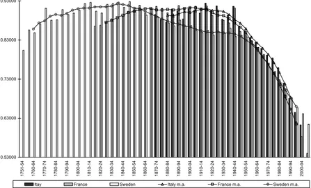
Figure 1 was constructed using the period life tables (both sexes) of three countries (Sweden, France, Italy) in which the beginning of the health transition can be said to have occurred at very different times. At the same time, relevant differences can be noted in the initial date of the continuous registration of deaths allowing the construction of life tables (1751 for Sweden, 1816 for France, 1872 for Italy).
If we observe the figure, we are struck by the fact that in all the three cases we can identify a first stage of increase of the mortality risks between 80 and 90 years. This phase is very precocious in Sweden (from the latest decades of the eighteenth century and up to about 1840). The second country which shows an initial increase in mortality at advanced ages is France, between about 1830 and 1870, but here a subsequent long phase of approximate stability can be observed before the start of the irreversible decline. Finally, starting only in the last decades of the nineteenth century, and lasting a considerably shorter period of time, the same increase can be shown for Italy too.
0.53000 0.63000 0.73000 0.83000 0.93000 17 51-54 17 60-64 17 70-74 17 80-84 17 90-94 18 00-04 18 10-14 18 20-24 18 30-34 18 40-44 18 50-54 18 60-64 18 70-74 18 80-84 18 90-94 19 00-04 19 10-14 19 20-24 19 30-34 19 40-44 19 50-54 19 60-64 19 70-74 19 80-84 19 90-94 20 00-04
Itay France Sweden Italy m.a. France m.a. Sweden m.a.
Figure 1 – Probability of dying between 80 and 90 years of age in Sweden (1751-2007), France
(1816-2004) and Italy (1872-2004).
As a matter of fact, the aim of this brief analysis concerning three European countries is simply to verify the possibility that in different contexts (both with regard to mortality factors and to the completeness and quality of the data which
5 The Human Mortality Database provides both abridged and complete life tables. We chose to use abridged life tables referred to every five calendar years, then we smoothed the values with a five-term moving average.
allow the construction of the life tables6), an initial increase in advanced age
mor-tality risks may actually be appreciated.
We shall now concentrate on the Italian case and analyse in more detail the trend of the mortality risks between 80 and 90 years of age from 1872 to 1922, illustrated in Figure 2. If we restrict the comparison to 1881-82 and 1900-01 (as we are obliged to if we use only the life tables constructed in census years) we ap-preciate a strong increase of 10q80 (this fact bears out data published many years
ago by Tizzano (1965) concerning the open class 75+). In fact the values of 1881 and 1882 are among the lowest of the whole period, while the values of 1900 and 1901 are among the highest. If we observe the whole series of the mortality risks, we have the idea of a very high variability. We can in any case also appreciate a moderate, growing trend of 10q80 between 1872 and 1922.
0.8500 0.8650 0.8800 0.8950 0.9100 0.9250 0.9400 18 72 18 74 18 76 18 78 18 80 18 82 18 84 18 86 18 88 18 90 18 92 18 94 18 96 18 98 19 00 19 02 19 04 19 06 19 08 19 10 19 12 19 14 19 16 19 18 19 20 19 22
Figure 2 – Probability of dying (both sexes) between 80 and 90 years of age in Italy from 1872 to
1922, according to HMD period life tables.
In general, we cannot exclude the existence of some factors that have actually contributed, in the last decades of nineteenth century and in the first decades of twentieth century, to the reduction of the survival probability of the elderly.
The difficulty in giving a plausible answer in this respect is linked to two dif-ferent problems. First, we ought to reconstruct, at least approximately, the whole life history (in terms of mortality risks) of the cohorts that were about 80 or 90 years old approximately between 1880 and 1900. Therefore, we are dealing with cohorts that were born at the beginning of the nineteenth century, whose com-plete cohort life table is impossible to reconstruct. Neither is it possible, for those cohorts, to estimate the percentage of surviving people up to 80 years. For this purpose, the level of l80 that we can draw from the period life tables is not
par-ticularly valuable.
6 The accuracy of ancient Swedish deaths and population registers and, in particular, the quality of age data are well illustrated by Lundström (1995).
On the other hand, we should investigate the main old age mortality causes at the end of the nineteenth century, as trying to explain the possible increases of mortality linked to the worsening of specific conditions. In Section 4 we shall outline the elderly cause specific mortality as far as the period we consider is con-cerned, but we have to consider, in this case as well, the poor quality of data.
For the sake of argument, we could assume that the very strong selection ef-fected by mortality from the very first instants of life and then through the whole course of life (Caselli et al., 2000; Vaupel and Yashin, 2006) might, in a very dis-tant past, have allowed only very few and highly select people to reach the threshold of old age. Those select individuals could have had a stronger resistance to mortality in the very old ages in comparison to more recent cohorts, when bet-ter conditions of life also enabled the achievement of very old ages to less strong individuals.
In fact, several important studies have discussed the possible debilitation or selec-tion effects of infant and child mortality levels on adult or elderly mortality. As far as the Italian case is concerned, we can cite the pioneer study of Livi Bacci (1962) and the one of Barbi and Caselli (2003). Both of them have faced the problem by analysing the regional differences in elderly mortality. In particular, Barbi and Caselli’s results and speculations are very stimulating7, but – as they recognize in
the discussion of the results (p. 52) – “whether it is the selection hypothesis rather than the debilitation hypothesis that has a role in differentiating mortality by region and sex is hard to identify, it being quite difficulty to distinguish between the ef-fects of selection or debilitation”.
Conversely, Caselli and Capocaccia (1989) deal with the debilitation and selec-tion role of early towards adult mortality at a naselec-tional level, in a cohort perspec-tive as well. Their analysis considers the Italian cohorts born between 1882 and 1953. As discussing the results of the application of a logistic regression model, they admit that the low mortality above 45 in the oldest cohorts (in comparison with the younger ones) may be caused “by their weakest members being lost through highly selective mortality in childhood and early adult life. By the same argument, the mortality of the younger cohorts could have been raised, because of their more favourable early mortality, which has resulted in a larger number of intrinsically weak survivors” (p. 151). Though the authors look very cautious about this hypothesis, a similar situation could be envisaged as far as the Italian cohorts which had reached an old age between 1881 and 1901 (the ones which were born in the first decades of the nineteenth century) are concerned.
Nevertheless, other hypotheses concerning the factors which may have caused the increase of the elderly mortality in the last decades of the Nineteenth Century could be considered. For instance, the agrarian crisis which significantly reduced the annual per capita calories in Italy for a period of about twenty years starting from the beginning of the Eighties, could have affected, year after year, the
7 Taking into account mortality experienced at earlier ages, Barbi and Caselli analyse the geographi-cal differences in mortality among the old and oldest old with reference to Italy and four representative regions (Lombardia, Toscana, Calabria and Sicilia), using longitudinal data obtained by mean of a very complex reconstruction of the mortality history of the cohorts born in 1891 and 1892.
est members of the population, that is to say the elderly. This is one of the possi-ble explanations of the higher level of elderly mortality risks registered in 1901 in comparison with 18818.
3. THE CONSTRUCTION OF REGIONAL LIFE TABLES: DATA RELIABILITY
In the period we considered (1881-1921), data published by Dirstat9 enable the
construction of regional life tables around the census years of 1881, 1901, 1911, 1921. With reference to 1921-22 we used the tables constructed by Gini and Gal-vani (1931). For the three previous periods we had at our disposal unpublished life tables which were constructed in more recent years by researchers10 of the
Department of Statistics of Bologna University11.
It is important to note that the measure of mortality risks in old ages is based on very scant amounts of living people and deaths. Moreover, as far as 1881-82 is concerned, the age distribution of the population (and also that of deaths) is quite inaccurate12.
In any case, the lack of annual age distributions (concerning sometimes the population age distributions, other times the death age distributions, more often both of them) obliges either to estimate the annual age distributions (Gini and Galvani chose this method) or to estimate five-year probabilities of death starting from five-year specific mortality rates. We chose the second way for the construc-tion of regional abridged life tables, since very similar results can be obtained both by the first or by the second procedure13, provided that age recording
(con-cerning population and deaths) is accurate.
The values for advanced age probabilities of death in the 1881-82 life tables must be considered with much more caution. In effect, the five-year age distribu-tion of populadistribu-tion in 1881 published by Dirstat shows very important irregulari-ties, especially as far as Southern regions are concerned, doubtless caused by a very inaccurate age statement on the part of the people surveyed. These
8 As a matter of fact, no clear relationship between the annual series of per capita calories and of mortality indicators can be detected for the period including the agrarian crisis (approximately 1880-1900), at least at the national level (Del Panta and Forini, 1994).
9 Dirstat is an acronym of “Direzione Generale di Statistica”, a section of the Ministry of Agri-culture whose task was the production of statistical data.
10 Under the responsibility of Lorenzo Del Panta.
11 Abridged regional life tables were constructed for 1871-72, 1881-82, 1900-01, 1910-12, 1921-22. The methodology (in particular for 1881-82 tables) is stated in Del Panta (1998).
12 Generally (apart from a few exceptions) Dirstat publications provide, until 1921, five year age distributions of population and deaths. It is important to note that, in census records, the year of birth was registered only starting from the 1901 census. Previously only age (in years of life) was registered. Therefore, in the 1881 census age statement is still approximate, and age heaping on ages ending in zero also distorts five-year age distributions (Preston et al. 1999).
13 The values of the probabilities of death drawn in our abridged life tables for 1921-22 are very similar, for all the Italian regions, to the values drawn in the complete life tables by Gini and Gal-vani. The estimate of the five-year probabilities of death has been obtained using the formula pro-posed by Reed and Merrell (1939).
larities lead to an overestimation of 5q75, not entirely counterbalanced by an
un-derestimation of 5q80 (Preston et al., 1999).
After several attempts to correct census year age distributions and five-year probabilities of death, we decided to undertake a different way and we con-structed from the beginning regional life tables for 1881-82, after having esti-mated annual distributions of population and deaths. As previously said, with ref-erence to 1881-82 only deaths and population data classified according to five-year age groups (up to the last open interval 100+) are available. Therefore, we split these grouped data into single year of age by applying a cubic spline to the cumulative number of deaths or individuals, in the following form (Mc Neil et al., 1977; Wilmoth et al., 2007): 2 3 3 0 1 2 3 1 ( ) ( n x i i i Y x x x x k I x
ki), (1)where Y is the cumulative number of deaths or individuals within year t up to x
age x; 0, , ,1 2 3, , ,...,1 2 n are the n+4 parameters that must be estimated;
( )
I is an indicator function and k k1, ,...,2 kn denote the so-called knots (for more
details, see Roli, 2008).
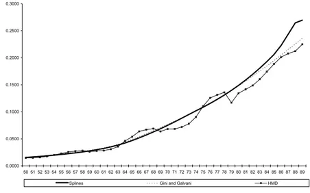
Let us now consider (Figure 3) the values of the annual probabilities of death between 50 and 90 years of age (both sexes) of the life table concerning the Ital-ian population (1881-82), which we have constructed using the procedure which has just been explained.
0.0000 0.0500 0.1000 0.1500 0.2000 0.2500 0.3000 50 51 52 53 54 55 56 57 58 59 60 61 62 63 64 65 66 67 68 69 70 71 72 73 74 75 76 77 78 79 80 81 82 83 84 85 86 87 88 89
Splines Gini and Galvani HMD
Figure 3 – Italy 1881-82. Annual probabilities of dying from 50 up to 90 years of age obtained by:
spline smoothing, Gini and Galvani’s tables and HMD tables.
If we compare these values with those drawn from the life table published by Gini and Galvani and with those of the life table (still for 1881-82) of the HMD,
we can easily see that the trend of the qx in our life table and the one in Gini and
Galvani’s table are almost the same up to about 80 years of age, but afterwards our life table suggests slightly higher values. The probabilities of death drawn from the HMD life tables show a rather irregular trend and, in any case, starting from 79 years of age they maintain significantly lower values in comparison both with our life table and with Gini and Galvani’s one.
Our belief is that the life tables hitherto at our disposal, which were con-structed around the 1881 census (both Gini and Galvani’s and HMD’s tables, as well as our previous life tables) underestimated mortality beyond 80 years of age, thereby exaggerating the actual increase of elderly mortality which characterizes the end of the nineteenth century.
Moreover, we must stress that, in our opinion, the degree of underestimation of the elderly mortality in 1881-82 varies substantially among Italian regions, and is found to be much stronger in the Southern regions, where the degree of irregu-larity in the age distribution of the population is substantially higher than the na-tional average. With regard to this, in Table 3 we show the regional values (1881-82) of 10q80 drawn from our new tables (which will be used in Section 5)
com-pared to the values of the previously constructed abridged tables14.
As already mentioned, for all the regions (save for Veneto) the values of the old tables look lower, but the differences between the old and the new tables are minimal in Northern regions and much higher in Southern regions, up to a maximum of 9 per cent in Sardegna.
In fact, the southern Italian regions (especially the ones towards the bottom of the table starting from Puglia) are characterized – as far as the 1881 census is concerned – by an abnormally low ratio between the population totals for the 75-79 and 80-84 age classes. This ratio (for males and females together) is about 1.75-79 for Italy on the whole, and varies, for southern regions, from 0.88 for Sicilia to 1.10 for Sardegna.
TABLE 3
Regional values of 10q80 (both sexes) in 1881-82: comparison between old life tables and new ones (splines) Old (abridged) life tables (1) New (complete) life tables (2) (2)/(1)
Piemonte 0.9363 0.9388 1.003 Liguria 0.8502 0.8612 1.013 Lombardia 0.9283 0.9281 1.000 Veneto 0.8982 0.8967 0.998 Emilia 0.8929 0.8934 1.001 Toscana 0.8903 0.8998 1.011 Umbria 0.8524 0.8726 1.024 Marche 0.8925 0.9058 1.015 Lazio 0.9077 0.9162 1.009 Abruzzi 0.8767 0.8897 1.015 Campania 0.8898 0.9095 1.022 Puglia 0.8419 0.8805 1.046 Basilicata 0.8555 0.8950 1.046 Calabria 0.8791 0.9073 1.032 Sicilia 0.8577 0.8976 1.047 Sardegna 0.7780 0.8485 1.091 ITALY 0.8803 0.9015 1.024 14 See footnote 11.
As far as 10q80 is concerned, for Italy on the whole the new estimate (0.915) is
2.4 per cent higher both in comparison with our old abridged tables and with Gini and Galvani’s tables, but the difference with the value (0.8625) drawn by the HMD tables (see again figure 2) is rather more evident (4.5 per cent).
4. A FIRST LOOK AT THE OVERALL ELDERLY SURVIVAL LEVEL IN ITALY AND IN THE ITALIAN REGIONS
Before undertaking a detailed statistical analysis of the chronological and terri-torial variations of elderly mortality in the forty years period between 1881 and 1921, we introduce some preliminary data, which provide the general framework of the phenomenon under observation.
Table 4 shows life expectancy at 70 years of age (both sexes) for each of the four dates in question.
It is important to note that, during the course of the forty years in question, the increase of this indicator is very slight (for Italy as a whole from 8.0 to 8.4). It is also interesting to observe that the geographical variability clearly decreases be-tween 1881 and 1921. Finally, we can see that various regions maintain the ex-treme positions in the regional ranking from the beginning to the end of the pe-riod: for instance, Puglia and Liguria are at all times among the regions showing a level well above the national average.
TABLE 4
Regional life tables (both sexes): life expectancy at 70 years of age and probablility of dying between 70 and 85 years (1881-1921) e70 15q70 1881 1901 1911 1921 1881 1901 1911 1921 Piemonte 7.37 7.61 8.15 8.40 0.9137 0.9154 0.8886 0.8748 Liguria 9.35 8.38 8.76 8.88 0.8124 0.8716 0.8521 0.8436 Lombardia 7.08 7.24 7.68 7.63 0.9132 0.9242 0.9066 0.9026 Veneto 7.98 8.39 8.72 8.86 0.8754 0.8704 0.8594 0.8490 Emilia 7.54 7.61 8.15 8.20 0.8909 0.9073 0.8883 0.8619 Toscana 8.40 7.77 8.26 8.22 0.8525 0.9109 0.8845 0.8829 Umbria 8.50 7.94 8.55 8.26 0.8480 0.8921 0.8720 0.8801 Marche 8.21 7.78 8.31 7.86 0.8740 0.9031 0.8858 0.8987 Lazio 7.42 7.47 7.92 7.85 0.8991 0.9190 0.8950 0.8951 Abruzzi 8.49 8.22 8.74 8.58 0.8528 0.8899 0.8617 0.8706 Campania 8.02 7.90 8.33 8.30 0.8729 0.9002 0.8784 0.8787 Puglia 8.77 7.90 8.88 8.70 0.8388 0.8972 0.8418 0.8564 Basilicata 8.34 7.64 8.48 8.07 0.8471 0.9103 0.8697 0.8890 Calabria 7.87 7.78 9.02 8.44 0.8674 0.9033 0.8331 0.8735 Sicilia 8.85 7.93 8.65 8.72 0.8238 0.8953 0.8598 0.8558 Sardegna 7.66 7.59 8.37 8.66 0.8807 0.9059 0.8733 0.8595 CV 0.0757 0.0401 0.0426 0.0448 0.0341 0.0166 0.0227 0.0204 ITALY 8.00 7.75 8.32 8.43 0.8588 0.9156 0.8729 0.8764
On the contrary, Lombardia and Lazio stand out with very low levels in all the dates. In Section 5 we will go back to some of these regional specificities.
In the same table we report the values of 15q70 of all the Italian regions. The
ra-tionale behind the choice of this indicator as an elderly mortality measure will be illustrated in Section 5.
Let us first consider the values of 15q70 for the Italian population as a whole: the
increase in mortality between 1881 and 1901, which we have already stressed, ap-pears clearly from these data. The later decrease (1901-11) of the mortality risk leads to a level of 15q70 stilla little higher then in 1881, while in 1921 the national
level of 15q70 is close to that of 1911.
If we focus our attention on the first interval (1881-1901), we can see that the mortality increase concerns all the regions (except Veneto) but has very different scopes. As we have already observed, the increase is generally bigger in the re-gions which in 1881 had lower mortality risks. Indeed, the variability sharply de-creases from the first to the second date. Finally, we can note that some regions (Lombardia in particular) maintain along the whole period elderly mortality risks well above the national average, while other regions, like Puglia and Liguria, show consistently lower levels of mortality in advanced age.
It is nevertheless difficult to add more specific remarks to this first brief obser-vation without undertaking a multivariate statistical analysis, which is the object of Section 5. We can, however, make some observations concerning the cause-specific mortality structure which characterized the Italian regions at the begin-ning of the period in question15. As a matter of fact, the distribution of deaths by
cause and age groups was published16 at regional level only for 1888. These data
allowed the calculation of cause-specific mortality risks17 for people aged 60 and
over. In Table 5, in the interest of space, we show the values of the rates for large classes of causes and only for four regions which have been chosen as examples. If we consider the values of the rates for Italy as a whole, we can first of all note that mortality caused by infectious diseases was still more than double in com-parison with that caused by cancers. At large, in comcom-parison with an overall rate of 74 (per thousand), we can see that the most important groups of causes were the respiratory diseases (nearly 20), and far behind the circulatory and nervous system diseases and senility.
We must stress in particular the high value of the rate attributed to “senility”, as this is a rough and generic definition which precludes any deeper regional analysis, since its value has a very variable level (from 16.2 attributed to Sardegna to 8.6 for Puglia). Despite these difficulties in the analysis, some regional speci-ficities seem noteworthy. For instance, if we compare the cause mortality struc-ture of Lombardia and Sardegna (the latter registers 4.2 points more than the former in senility), we note that Lombardia has higher values for cancers (2.3 points more) and especially for the circulatory system diseases18 (11.2 points
more). For malaria, on the other hand, Sardegna (and at a minor level also Puglia)
15 A detailed analysis of the cause-specific mortality structure (without the specification of the age of death) of the Italian regions since the last decades of the nineteenth century and until the end of the First World War was carried out by Mortara (1925). More recently, Pozzi (2000) analysed the evolution of the cause mortality structure in Italy at provincial level. See also Caselli (1990).
16 Ministero di agricoltura, industria e commercio (1890).
17 The population above 60 was estimated for 1888 on the basis of the age distributions of population in 1881 and 1901.
18 We can remember that Caselli and Lipsi (2006) attribute mainly to low levels of circulatory diseases mortality the significant longevity of Sardinians contemporary males.
shows very high values, while this cause of death is nearly absent in Lombardia and in Veneto. Finally, in the latter a noteworthy mortality risk can be attributed to pellagra.
TABLE 5
Cause specific mortality rates above 60 years (both sexes) per 1000 inhabitants in Italy and in four regions, 1888
ITALY Lombardia Veneto Puglia Sardegna
infectious and parasitic diseases 4.6 3.0 3.4 6.1 8.8
typhoid fever 1.0 0.6 0.8 1.4 0.7
malaria 0.9 0.2 0.2 1.7 2.8
dysentery 0.6 0.1 0.1 0.7 1.4
tuberculosis (all types) 1.2 1.2 1.3 1.3 1.9
neoplasms 2.2 3.1 2.2 1.6 0.8
malignant neoplasms of the stomach 0.6 1.1 0.5 0.3 0.1
rheumatic, nutrition and endocrine glands diseases 1.3 2.2 3.2 0.7 1.0
pellagra 0.7 1.7 2.8 0.0 0.0
nervous system diseases 10.9 13.0 11.1 10.0 8.5
stroke of apoplexy and cerebral congestion 9.1 10.8 9.2 8.5 7.0
diseases of the circulatory system 11.3 15.9 13.6 9.0 4.7
heart diseases 9.6 14.0 10.5 7.5 3.6
diseases of the respiratory system 19.9 17.0 17.5 21.3 20.4
bronchial tubes diseases 6.2 5.2 6.6 6.0 3.9
acute pneumonia 9.9 7.7 8.0 12.0 9.6
diseases of the digestive system 7.2 6.6 5.4 7.0 11.6
enteritis and diarrhoea 4.0 3.4 2.9 4.3 6.2
senility 11.3 12.0 10.2 8.6 16.2
other causes 3.3 3.3 2.9 2.7 3.3
unspecified causes 2.0 1.4 1.5 1.1 3.4
all causes of death 74.0 77.5 71.0 68.0 78.6
Going back to malaria, it is noteworthy to remark that, considering the gender differences in the mortality risks (for all causes) between 80 and 90 years of age in the Italian regions in 1881-82 (Table 6), we can observe very similar values with the exception of the regions where malaria had the highest mortality levels.
TABLE 6
Probability of death between 80 and 90 years (by sex) in Italian regions, 1881-82
m f Piemonte 0.9365 0.9415 Liguria 0.8633 0.8596 Lombardia 0.9274 0.9290 Veneto 0.8941 0.8991 Emilia 0.8932 0.8941 Toscana 0.8954 0.9049 Umbria 0.8687 0.8797 Marche 0.9175 0.8954 Lazio 0.8964 0.9317 Abruzzi 0.8804 0.8997 Campania 0.9014 0.9169 Puglia 0.8475 0.9048 Basilicata 0.8957 0.8945 Calabria 0.8895 0.9220 Sicilia 0.8741 0.9163 Sardegna 0.8369 0.8614 ITALY 0.8956 0.9074
In these regions, where in adult ages a prevalence of male mortality can be ap-preciated in the last decades of the nineteenth century (Del Panta and Rosina,
200219; Angeli and Salvini, 2001), we could perhaps assume a selection effect of
malaria which allows only very strong and resistant males to survive up to 80 years of age, and these therefore show a higher resistance in comparison with fe-males between 80 and 90 years of age.
After these introductory remarks, let us turn to a statistical analysis of regional differences in elderly mortality.
5. A MULTI-WAY ANALYSIS OF ELDERLY SURVIVAL INDICATORS IN ITALIAN REGIONS ACROSS 1881-1921: THE STATIS METHOD
The STATIS method (Structuration des Tableaux A Trois Indices de la Statis-tique) has been introduced by Escoufier (1973, 1980), with the aim of exploring three-way data, handled as a set of K matrices, by computing Euclidean distances between configurations of points (see, for example, Lavit et al., 1994). As far as the present analysis is concerned, it allows to accomplish the following tasks: 1) Comparing the K configurations (see subsection 5.1):
to compare the configurations of the points (observations) in the K settings by analyzing their similarity structure, with the aim of investigating a possible rela-tionship among them.
2) Identification and analysis of the “compromise” (see subsection 5.2):
to combine the configurations into a common representation of the observations, called “the compromise”. It is analyzed via principal component analysis, whose components can be interpreted through their correlations with the original vari-ables observed in the various settings.
3) Exploring the common structure (see subsection 5.3):
to project the units onto the space spanned by the main components (dimen-sions) of the compromise, in order to analyze communalities and discrepancies. 4) Exploring across setting discrepancies (see subsection 5.4):
for each pair of settings, compute the contribution of each unit to the distance between the settings, in order to detect the units that mostly varied their position across the K configurations.
Some multi-way analysis methods, like the so-called Tucker3 model, are based on flexible models allowing to explore each of the three modes (that is, observa-tions, variables and settings) simultaneously; on the contrary, STATIS analyzes the three-way array as a set of K slice matrices unitsvariables20. We used STATIS
be-cause it is an exploratory method, thus being the most natural candidate for applica-tions, like the present one, where no true stochastic framework can be formulated.
19 Del Panta and Rosina attribute to malaria the adult (15-70 years) male higher mortality in the southern Italian regions.
20 The similarities among these matrices are taken into account in determining the contribution of each matrix to the “compromise”. As an example of a different approach, still applied to multi-way demographic data, see Bellini et al. (1992).
The data have been arranged as a three-way array with modes regions
variablesoccasions, where:
variables correspond to 8 demographic indicators: besides e0, which attests
to the overall survival level of the regions, we selected several indicators as best representing the elderly survival: e70, ex=10, e90, 5q70, 5q75, 5q80 e 5q85;21
occasions are the 4 census years, at the turn of the nineteenth century: 1881, 1901, 1911, 1921.
Italy was considered as a supplementary unit, namely it was ignored when per-forming the analysis but it was plotted onto the compromise, as well as the 16 re-gions.
Therefore, the data are stored as 4 separate matrices, X1, …, X4, each
consist-ing of the measurements of the same 8 variables on the same 16 units taken at a different occasion. For each separate occasion, the data (stored in the generic ma-trix Xk) have been standardized: in this preprocessing phase, observations were
weighted in order to take into account their different population amount (the weights, summing to 1, were computed on the basis of the 1901 census data).
The following phases of the method have been carried out using two distinct options about the weights of the regions, stored in the diagonal matrix D: the former was to assign identical weights (that is, D=I, with I denoting the identity matrix), the latter was to assign the same weights used in the preprocessing phase. The two options yielded similar solutions, but the former gave rise to neater re-sults which are reported and commented in the following. We note that when uniform weights are assigned to the regions, it means that one is interested in de-tecting any regional pattern, whatever the size of the region.
The analysis has been carried out using R (http://cran.r-project.org/) and SPAD software, version 5.0 (SPAD, 1997; http://www.cisia.com).
5.1. Comparing the configurations
A pairwise comparison of the configurations corresponding to the 4 occasions is performed by means of the so-called RVcoefficients:
' , ' 2 2 ' trace( ) trace( ) trace( ) t t t t t t RV S DS D S D S D , (2)
21 With regard to the elderly survival indicators, we included the age at which remaining life ex-pectancy is ten years (ex=10), which is considered the threshold of the beginning of old age (be-tween 65 and 68 years, both for males and females, in the period under observation), together with the life expectancy at the beginning and at the end of the period of life (70-90 years of age) on which we decided to focus (see section 2). Within that life span, we considered the four distinct five-yearly probabilities of death, by which a more detailed analysis of elderly mortality can be car-ried out.
We decided to include the general survival level (e0) because its presence turned out not to alter the results (as it could be expected, since it is not an elderly survival indicator) but proved to be relevant in the interpretation of the “compromise”.
where the scalar product matrix St X Xt tT( , ' 1,...,4t t ) gives a representation
of the mutual relationships (in terms of Euclidean distances) among the regions at occasion t on the basis of the observed variables, and D is a diagonal matrix
as-signing weights to the regions; from here on, D is taken to be equal to the
iden-tity matrix. RVt,t’ gives the cosine between the matrices S e t S , taken in vector-t'
ized form; therefore, it takes its maximum value (=1) if the compared configura-tions are identical.
The RV coefficients for the four occasions are reported in Table 7. The results show that a common structure among the four occasions is present, which justi-fies their simultaneous analysis. In addition, the RV coefficient values are moder-ately high and decrease with increasing time lag: this suggests that both common and specific features are worth to be analysed.
TABLE 7 RV coefficients 1881 1901 1911 1921 1881 1 1901 0.582 1 1911 0.524 0.591 1 1921 0.389 0.567 0.564 1
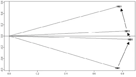
The similarity structure of the four scalar-product matrices, called interstruc-ture, can be visually analyzed by the eigen-decomposition of the between-occasion cosine matrix C=[RVt,t’]: occasions are represented as points in the ei-genspace. Concerning the data shown in Table 7, the bivariate representation spanned by the first two principal components is reported in Figure 4. The sum of the corresponding two eigenvalues is about 80% of the overall sum of the ei-genvalues.
The most relevant result visible in the plot is that occasions are nicely ordered in temporal sequence. This means that the structure shared by the occasions changed according to a temporal pattern. It provides an important confirmation to the soundness of the analysis, since the chronological ordering of the four oc-casions is not contained in the data as “a priori information”.
5.2. Identification and analysis of the “compromise”
The so-called “compromise”, S, is a weighted average of the scalar-product
matrices representing each occasion; the weights are chosen so that configura-tions agreeing most with other configuraconfigura-tions will have the larger weights (for further details, see Lavit et al., 1994). By applying the singular value decomposi-tion S=QLQT, with QTDQ=I, the compromise space can be approximated by
considering only the most relevant columns of the matrix Q.
In the present analysis, the approximation of the compromise provided by the first two principal components explains almost the 70% of the inertia. After re-stricting attention to the first five components, Table 8 presents the (cumulated) percentage of explained inertia.
TABLE 8
(Cumulated) percentage of inertia explained by the first five principal components Dimension Percentage of inertia Cumulated percentage of inertia
1 43 43 2 23 67 3 9 76 4 8 84 5 5 89
The two extracted components can be interpreted by analyzing the values of their correlation coefficients with the original variables observed in the various settings (see Table 9). In fact, these correlations are nothing but the coordinates of the original variables onto the compromise.
The first dimension (accounting for 43% of the inertia) can be interpreted as the opposition of indicators e70 and ex=10 (on the right hand side) to the mortality
indicators (on the left hand side). This result sounds reasonable, since:
1) indicator ex=10 can be liken to e70, since it takes values around 70 in all the
four occasions under investigation. In fact, the correlation between ex=10 and e70
exceeds 0.93 in all occasions;
2) life expectancy at age 70 globally describes the survival levels after this age; therefore, it is expected to grow with decreasing values of the mortality risks after age 70.
As a consequence, the first dimension can be interpreted as an overall indicator of old people survival/mortality.
The second dimension (accounting for 23% of the inertia) represents a con-trast between e0 (on the right hand side) and e90 (on the left hand side), with the
only exception of variable e90 in occasion 1921 which shows a slight correlation
TABLE 9
Correlations of the original variables with the first two dimensions of the compromise
1881 1901
Dim. 1 Dim. 2 Dim. 1 Dim. 2
e0 0.227 0.590 0.044 0.925 e70 0.837 0.034 0.874 0.405 e90 0.237 -0.771 0.206 -0.826 ex=10 0.721 0.202 0.846 0.424 5q70 -0.702 -0.296 -0.735 -0.599 5q75 -0.825 0.049 -0.914 -0.232 5q80 -0.778 0.386 -0.797 -0.160 5q85 -0.440 0.130 -0.383 0.736 1911 1921
Dim. 1 Dim. 2 Dim. 1 Dim. 2
e0 -0.053 0.778 -0.014 0.902 e70 0.913 -0.070 0.880 0.049 e90 0.266 -0.768 0.258 -0.229 ex=10 0.899 -0.016 0.892 0.075 5q70 -0.904 -0.013 -0.862 -0.092 5q75 -0.803 -0.161 -0.823 -0.083 5q80 -0.791 0.410 -0.803 0.083 5q85 -0.600 0.353 -0.556 0.278
This opposition is confirmed by the negative values of the correlation coeffi-cient between e0 and e90 in the four studied occasions (the correlation coefficient
is equal to -0.236 in 1881, -0.668 in 1901, -0.535 in 1911 and -0.142 in 1921). At first sight, the opposition of these indicators along the second component seems unexpected, since they both are survival indicators. More specifically, life expec-tancy at birth summarizes the overall survival level across all age groups (in the period under investigation, due to high infant mortality rates, it is highly sensitive to the rate of death in the first few years of life), whereas e90 reflects the mortality
level of very old people.
A tentative explanation could be given by conjecturing once again a kind of se-lection effect, as discussed in Section 2: it could be argued that, under low overall survival levels, only a few selected individuals can reach old age, thus producing relatively high values of old age survival probabilities. This interpretation needs some caution since it must be stressed that the observed demographic indicators are computed on the basis of cross-sectional mortality tables; they do not come from the longitudinal study of a generation until the end, hence they show a pic-ture resulting from very heterogeneous patterns and experiences.
5.3. Exploring the common structure
The coordinates of the regions onto the compromise are computed through the matrix F=QL1/2 and represent the position of the regions in the common
structure shared by the different occasions. They are shown in Figure 5.
It is worth noting that Italy (Regno), which has been projected as well as a supplementary unit, is placed near the origin of the axes, as it could be expected since Italy summarizes the different demographic patterns of the 16 regions.
The positions of the regions can be interpreted on the basis of the interpreta-tion of the axes given in Secinterpreta-tion 5.2. Lombardia and Lazio are placed as extreme
Figure 5 − Projections of the regions on the bivariate approximation of the compromise.
points in the negative half-plane of the first dimension: this means that, in the 40 year period we considered, they are characterized by the lowest old age survival levels. On the opposite side, Liguria, Veneto and Puglia come out among the most favourite regions in terms of longevity. These patterns are visible also by comparing the regions with respect to the values of e70 and 15q70, reported in
Ta-ble 4, that can be deemed to represent the first dimension in its positive and negative senses, respectively22 (as illustrated in Secion 5.2). In fact, Liguria and
Puglia stand out as the regions where life expectancy at age 70 mostly exceeds the national value, taking the 40 year period under investigation as a whole; on the other hand, by considering their average behaviour as before, these regions are best ranked in terms of 15q70. On the contrary, Lombardia and Lazio are, on
aver-age, the most disadvantaged regions with respect to old people survival.
If we focus attention on the interpretation of the second dimension, it can be seen that Basilicata, Puglia and Sardegna are placed in the lowest part of the plot, well separated from the remaining regions. This suggests that, in the common space given by the compromise, these regions have the best performance in terms of very old people life expectancy, while being mostly disadvantaged as far as overall survival levels are concerned. In the latter respect, this result is coherent with the well known fact that Southern and Insular Italian regions (with the par-tial exception of Sardegna) have been characterized for a long time by higher lev-els of infant and child mortality with respect to Central and North regions. 5.4. Exploring across-setting discrepancies
A simple and immediate way to describe the across-setting discrepancies and to highlight which units they are mostly due to, is to project each scalar-product
22 It is worth mentioning that the latter indicator was preferred to 20q70 because the probability of death between ages 85 and 90 years are only slightly related to the considered dimension (see Table 9).
matrix St onto the compromise. In the resulting plot the dynamic followed by each region across occasions can be graphically described as a trajectory and can be interpreted w.r.t. the dimensions defining the common space. However, this approach yields good results only if the compromise is a good representative of all the configurations corresponding to the different occasions, that is, if all the RV coefficients are near to 1 (see Bolasco, 1999).
A different approach, which is valid under any condition, is to decompose the discrepancy between occasions t and t’ (t ≠ t’ ) into the contributions given by the different units. More precisely, the contributions given by the different units to the squared distance between the configurations St and St’ are contained in 16-dimensional vector dist : t t, '
2 ' , ' 2 ' diag[( ) ] , trace[( ) ] t t t t t t S S D dist S S D (3) where 2 trace( ) t t t S S S D . (4)
Unlike the “graphical approach”, based on trajectory plotting, this solution yields exact results, since the decomposition in (3) is based on algebraic calculus.
In the present application, this decomposition yields a set of 4×(4-1)/2 vectors that allows to detect which units are perturbed when passing from one occasion to another. Due to the temporal sequence of occasions, only pairs of contiguous occasions have to be considered. Results are reported in Table 10. In the follow-ing, only the most relevant contributions will be highlighted and commented. For better readability, the features emerged through these analyses will be also shown in terms of trajectories, being aware that trajectories represent an approximation of such patterns.
TABLE 10
Percent contributions of the regions to the discrepancies between contiguous occasions
1881-1901 1901-1911 1911-1921 Piemonte 5.61 3.90 7.14 Liguria 8.24 7.03 5.54 Lombardia 9.76 12.14 13.79 Veneto 18.35 8.65 7.29 Emilia 3.05 2.66 1.21 Toscana 3.73 1.60 0.87 Umbria 3.30 2.92 2.74 Marche 3.13 2.60 6.31 Lazio 5.43 5.56 4.47 Abruzzi 6.49 4.59 1.42 Campania 1.86 2.60 2.22 Puglia 4.93 11.04 12.34 Basilicata 6.23 8.51 7.10 Calabria 1.10 19.76 18.74 Sicilia 6.60 1.59 4.46 Sardegna 12.20 4.86 4.36
An important caveat that must be taken into account when interpreting the changes of a given region across the years is that these changes are referred to the overall dynamic of the phenomenon, because the method works on centered data matrices (which have been referred to as X1,…, X4 in Section 5.1). This implies
that, for example, a high contribution of a unit could be due to the fact that this unit remains quite stable despite the whole phenomenon is highly dynamic.
For the purpose of commenting the relevant contributions as deviation from the overall dynamic of elderly mortality, in the following we will resort to the data in Table 4, which provide synthetic information about the first (and main) dimen-sion of the compromise.
In light of the results in Table 10, the regions showing the most relevant con-tributions are Veneto, as far as the comparison between occasion 1881 and occa-sion 1901, and Calabria, for both the remaining comparisons. It is worth noting that each of these three contributions is above the threshold Q31,5(Q3Q1), where Q and 1 Q respectively denote the first and third quartile of the elements 3 in the corresponding vector distt t, '. This confirms the relevance of the above mentioned contributions.
In effect, Veneto represents an exception to the overall dynamic followed by Italian old people mortality between 1881 and 1901. As it has been already de-scribed in Section 2, in that period of time the probability of dying between ages 70 and 90 years underwent a considerable increase. Conversely, Veneto is the only region where 15q70 does not increase; moreover, among the few regions
showing some increase in life expectancy at age 70, it stands out with the highest gain (see Table 4). This is confirmed by inspecting the trajectories of the regions across 1881 and 1901, which can be drawn by comparing the two upper panels of Figure 6. In 1881, Veneto is placed near the origin along the first dimension, which means that it shares the national levels of old age survival. In 1901, it moves to the outermost position in the positive half-plane, thus revealing its rela-tive advantage with respect to the overall pattern.
Since the early twentieth century old age survival starts going up again, al-though only slightly: in particular, life expectancy at age 70 follows a slight posi-tive trend (see Table 4) while e90 remains quite stable. These considerations
should be taken into account when interpreting the results dealing with the com-parison between 1901 and 1911 and the one between 1911 and 1921. Throughout both these periods, Calabria is the region that mostly contributes to the distances between contiguous occasions.
Concerning the changes between 1901 and 1911, Calabria is characterized by the highest increase in the values of e70, while moving from average levels to the
lowest ones with respect to 15q70 (see Table 4). This is confirmed by inspecting the
trajectories of the regions across 1901 and 1911, obtainable by comparing the up-per right and the lower left panels of Figure 6. In 1901, Calabria is placed near the origin along the first dimension, whereas in 1911 it takes the rightmost position in the positive half-space. Turning back to Table 4, we can see that the remaining southern regions share a similar trend along the first axis, which however is less
pronounced than the one of Calabria; Campania represents an exception, since, like in the northern regions, its improvement in old age survival is less than the one registered in the whole nation.
Figure 6 − Projections of the regions on the compromise in each occasion: Piemonte (PI), Liguria
(LI), Lomabrdia (LO), Veneto (VE), Emilia (EM), Toscana (TO), Umbria (UM), Marche (MAR), Lazio (LA), Abruzzi (AB), Campania (CAM), Puglia (PU), Basilicata (BA), Calabria (CAL), Sicilia (SI) and Sardegna (SAR).
In the ten-years between 1911 and 1921, Calabria shows the most relevant contribution, once again, although in the opposite direction (see the two lower panels in Figure 6). In particular, as shown by the data reported in Table 4, it shows the greatest decrease in old age survival indicators: more precisely, the highest increment in the values of 15q70 is registered, while the levels of e70 show
the highest decrease. However, the modifications observed in Italian regions dur-ing this time interval are only very slight, in absolute terms, and the patterns of old age mortality can be deemed to be quite stable.
Finally, it is worth noting that the above-mentioned trajectories involve mainly the first dimension of the compromise. This is not surprising, since the second one accounts for only the 23% of inertia. In addition, it can be observed that the second dimension becomes less and less important throughout the occasions: by comparing the panels in Figure 6, a sort of “flattening trend” is visible, i.e. the points tend to become more scattered along the first axis than along the second one. As a consequence, the differences with respect to the second axis become less relevant in the interpretation of the results.
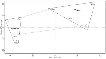
Before concluding, it can be interesting to compare the trajectories drawn by Lombardia and Veneto, plotted in Figure 7.
It can be pointed out that the corresponding convex hulls do not intersect, with Lombardia on the left and Veneto on the right. This confirms that in these regions the levels of elderly mortality are different from each other, and that the discrepancy gets larger during the period under investigation. More specifically, in 1881 Lombardia is ranked in the lowest positions as far as elderly survival levels are concerned, while Veneto is in line with national values; after 40 years, Lom- bardia remains quite stable around the relatively low initial values, while Veneto augments its advantage.
Figure 7 − Trajectories drawn by Lombardia and Veneto.
6. CONCLUDING REMARKS
While many authors have analyzed in detail, with reference to Italy, the chronological trend and the territorial differences of child and adult mortality at the beginning of the health transition, little attention has been paid up to now to the characteristics of elderly mortality.
In this paper, we focused our attention on the increase of elderly mortality at the beginning of the health transition (1881-1901) and on the possibility that it is partly due to the inaccuracy of the data. New complete regional life tables for 1881 were constructed by splitting five-year distributions of population and deaths using spline interpolation. On the new tables the increase of elderly mor-tality between 1881 and 1901 was still evident but had a minor size, especially for Southern regions, whose census and death age distributions are less accurate. Such a feature and the results of the multiway analysis carried out on the data were tentatively explained by resorting to the so-called selection hypothesis (that is, some individuals are frailer than others, and the frailer die first). This hypothesis was found to be a possible partial explanation of both territorial and chronologi-cal differences in elderly mortality.
A far as the territorial differences are concerned, our study highlighted the permanence for some regions of relatively high/low levels of elderly mortality (namely, Liguria and Puglia on one side and Lombardia and Lazio on the other one). Moreover, Veneto resulted to be atypical with regard to both data quality and the elderly mortality trend between 1881 and 1901.
These results could be the starting point for further investigations at a regional level aiming at revealing the causes of such differences. For example, an insight in cause-specific mortality of Sardegna pointed out that this region stands out in 1888 for extremely low values of mortality for circulatory system diseases. This fact can be related to the relatively low elderly mortality of contemporary Sardin-ian males observed by Casellli and Lipsi (2006).
Dipartimento di Scienze Statistiche LORENZO DEL PANTA
Alma Mater Studiorum – Università di Bologna DANIELA G. CALÒ LAURA M.B. BELOTTI
REFERENCES
A. ANGELI, S. SALVINI (2001), Mortalità per genere e salute riproduttiva: il percorso italiano tra
Otto-cento e NoveOtto-cento,in “Popolazione e Storia”,1,71-106.
E. BARBI, G. CASELLI (2003),Selection effects on regional differences in survivorship in Italy, “Genus”,
LIX (2), 37-61.
P. BELLINI, G. DALLA ZUANNA and M. MARSILI (1992),Trends in geographical differential mortality in
Italy (1970-90): tradition and change, “Genus”, XLVIII (1-2), 155-182.
S. BOLASCO (1999), Analisi multidimensionale dei dati. Metodi, strategie e criteri d'interpretazione, Ca-rocci, Roma.
G. BOVE, A. DI CIACCIO (1994) A user-oriented overview of multiway methods and software, “Compu-tational Statistics and Data Analysis”, 18, 15-37.
G. CASELLI (1990),Mortalità e sopravvivenza in Italia dall’Unità agli anni ’30, in SIDES,
“Popo-lazione, società e ambiente. Temi di demografia storica italiana (secc. XVII-XIX)”, Bo-logna, CLUEB, 275-309.
G. CASELLI (1991), Health Transition and the Cause-Specific Mortality, in R. Schofield, D. Reher, A. Bideau (editors), “The Decline of Mortality in Europe”, Oxford, Clarendon Press, 68-96.
G. CASELLI (2007),Mortalità degli adulti e differenze di genere nella prima fase della transizione
sani-taria, in M. Breschi, L. Pozzi (editors), “Salute, malattia e sopravvivenza in Italia tra
‘800 e ’900”, Udine, Forum, 293-310.
G. CASELLI, R. CAPOCACCIA (1989),Age, Period, Cohort and Early Mortality: an Analysis of Adult Mortality in Italy, in “Population Studies”, 43 (1), 133-153.
G. CASELLI, R.M. LIPSI (2006),Survival differences among the oldest old in Sardinia: who, what, where,
and why?, in “Demographic Research”, vol. 14, art. 13, 267-294.
G. CASELLI, J.W. VAUPEL and A.I. YASHIN (2000), Longevity, Heterogeneity, and Selection, in “Atti della XL Riunione Scientifica della Società Italiana di Statistica”, Istituto Nazionale di Statistica.
A.J. COALE, E.E. KISKER (1986),Mortality Crossovers: Reality or Bad Data?, in “Population
Stud-ies”, vol. 40, n. 3, 389-401.
La situazione in Italia, in SIDES, “Popolazione, società e ambiente. Temi di demografia
storica italiana (secc. XVII-XIX)”, Bologna, CLUEB, 245-273.
L. DEL PANTA (1998), Costruzione di tavole di mortalità provinciali abbreviate 1881/82, in “Bollet-tino di Demografia Storica”, 29, 61-69.
L. DEL PANTA, M.E. FORINI (1994), Disponibilità alimentari e tendenze della mortalità in Italia: un
tenta-tivo di analisi per il periodo 1861-1921, in “Bollettino di Demografia Storica”, 20, 111-121.
L. DEL PANTA, A. ROSINA (2002),Mortalità adulta per genere in Italia prima di Pasteur: variabilità
territoriale ed ipotesi esplicative, in L. Del Panta, L. Pozzi, R. Rettaroli, E. Sonnino (editors),
“Dinamiche di popolazione, mobilità e territorio in Italia, secoli XVII-XIX”, Forum, Udine, 181-196.
Y. ESCOUFIER (1973), Le traitement des variables vectorielles,“Biometrics”,29,751-76.
Y. ESCOUFIER (1980), L’anayse conjointe de plusieurs matrices de données, in M. Jolivet (Ed.), “Biométrie et Temps”. Paris: Société Francaise de Biométrie, 59-76.
C. GINI, L. GALVANI (1931),Tavole di mortalità della popolazione italiana, in “Annali di Statistica”, serie VI, vol. VIII, 1-412.
V. KANNISTO (1999),Assessing the Information on Age at Death of Old Persons in National Vital
Statistics, in B. Jeune and J.W. Vaupel (editors), “Validation of Exceptional Longevity”,
Odense Monographs on Population Aging 6, Odense University Press, Odense, 235-249.
C. LAVIT, Y. ESCOUFIER, R. SABATIER and P. TRAISSAC (1994),The ACT (STATIS method),
“Compu-tational Statistics and Data Analysis”, 18, 97-119.
L. LEBART, A. MORINEAU and M.PIRON (1995), Statistique exploratoire multidimensionnelle, Dunod, Paris.
M. LIVI BACCI (1962),Alcune considerazioni sulle tendenze della mortalità senile e sull’eventuale influen-
za selettiva della mortalità infantile, in “Rivista Italiana di Economia, Demografia e Stati-
stica”, XVIII (3-4), 60-73.
H. LUNDSTRÖM (1995),Record Longevity in Swedish Cohorts Born since 1700, in B. Jeune and J.W. Vaupel (editors), “Exceptional Longevity: from Prehistory to the Presen”, Odense Monographs on Population Aging 2, Odense University Press, Odense, 67-74.
D.R. MCNEIL, T.J. TRUSSELL and J.C.TURNER (1977), Spline interpolation of demographic data, “De-mography”, 14, 245-252.
MINISTERO DI AGRICOLTURA, INDUSTRIA E COMMERCIO, DIREZIONE DELLA STATISTICA GENERALE (1890),Statistica delle cause delle morti 1888, Roma, Tipografia Bodoniana.
G. MORTARA (1925), La salute pubblica in Italia durante e dopo la guerra, Bari, Laterza.
L. POZZI (2000), La lotta per la vita. Evoluzione e geografia della sopravvivenza in Italia fra ’800 e
’900, Udine, Forum.
S.H. PRESTON, I.T. ELO, Q. STEWART (1999),Effects of age misreporting on mortality estimates at older ages, in “Population Studies”, 53, 165-177.
L.J. REED, M. MERRELL (1939),A Short Method for Constructing an Abridged Life Table, in “Ameri-can Journal of Hygiene”, XXX, 2, 33-62.
R. RETTAROLI, G. ROLI, A. SAMOGGIA (2009), Health transition in adult and old ages: Italian
exam-ples, “Statistica”, LXIX, 1, pp. 89-111.
G. ROLI (2008), An adaptive procedure for estimating and comparing the old-age mortality in a long
his-torical perspective: Emilia-Romagna, 1871-2001, Quaderni di Dipartimento, Dipartimento
di Scienze Statistiche, Università di Bologna.
N.B. RYDER (1975), Notes on Stationary Populations, in “Population index”, vol. 41, n. 1, 3-28. SPAD (1997), SPAD TM. Analyse des Tableaux Multiples. Manuel de reference, CISIA, Paris. A.R. THATCHER (1992), Trends in Numbers and Mortality at High Ages in England and Wales, in
A. TIZZANO (1965),Mortalità generale, in “Annali di Statistica”, serie VIII, vol. 17, Roma,
Isti-tuto Centrale di Statistica, 441-465.
J.W. VAUPEL, A.I. YASHIN (2006), Unobserved population heterogeneity, in “Demography: analysis and syinthesis; a treatise in population studies” (Eds: G. Caselli, J. Vallin and G. Wunsch), vol. 1, Academic Press, London.
J.R. WILMOTH, K. ANDREEV, D. JDANOV, D.A. GLEI (2007), Methods protocol for the Human Mortality
Database, http://www.mortality.org.
SUMMARY
Elderly mortality in Italian regions at the beginning of the health transition (1881-1921)
The paper aims to highlight and analyze possible regional patterns of mortality at ad-vanced age (70-90 years) in Italy at the turn of the nineteenth century. The available data are referred to four distinct occasions, namely 1881-82, 1900-01, 1911-12 and 1921-22. After focusing attention on several elderly mortality indicators, we propose to analyze the resulting three-way array (with modes regionsindicatorsoccasions) using the STATIS method. As a critical preliminary step, new regional life tables for 1881-82 are constructed in order to reduce the possible bias due to the inaccuracy of the age distribution of the population and of the deaths in 1881. The resulting life tables are compared with Gini and Galvani’s ones and those available in the Human Mortality Database.