Accuracy Comparison between Techniques for the Establishment of Calibration Intervals: Application to Atomic Clocks

UNIVERSITY

OF TRENTO

DEPARTMENT OF INFORMATION AND COMMUNICATION TECHNOLOGY

38050 Povo – Trento (Italy), Via Sommarive 14

http://www.dit.unitn.it

ACCURACY COMPARISON BETWEEN TECHNIQUES FOR THE

ESTABLISHMENT OF CALIBRATION INTERVALS :

APPLICATION TO ATOMIC CLOCKS

David Macii, Patrizia Tavella, Elena Perone, Paolo Carbone, Dario Petri

January 2004

Accuracy Comparison between Techniques for

the Establishment of Calibration Intervals:

Application to Atomic Clocks

D. Macii

, Student Member, IEEE, P. Tavella

, E. Perone

,

P. Carbone

, Associate Member, IEEE, D. Petri

, Member, IEEE

1

DIEI – Dipartimento di Ingegneria Elettronica e dell’Informazione University of Perugia, via G. Duranti 93 – 06125 Perugia, Italy

Phone: +39 075–5853629, Fax: +39 075–5853654, E-mail: macii@diei.unipg.it, carbone@diei.unipg.it

2

Istituto Elettrotecnico Nazionale (IEN) “Galileo Ferraris”, *Guest scientist Strada delle cacce, 91 – 10135 Torino, Italy

Ph.: +39 011 3919235 – Fax: +39 011 3919259 – E-mail: tavella@tf.ien.it.

3

DIT, University of Trento, Via Sommarive, 14 – 38050 Trento, Italy

Ph.: +39 0461 883902 – Fax: +39 0461 882093 – E-mail: petri@dit.unitn.it.

Abstract

This paper deals with two different techniques for the establishment of the optimal calibration intervals of Cesium atomic clocks. In particular, the intervals obtained using a mathematical model derived from a metro-logical analysis are compared with those calculated with an iterative technique referred to as Simple Re-sponse Method (SRM). The remarkable consistency between the results achieved with these different calibra-tion strategies not only provides an experimental cross-validacalibra-tion of both techniques, but it also allows the definition of two interchangeable criteria to ensure the metrological confirmation of any atomic clock of this type.

Index Terms

Calibration intervals, Cesium atomic clocks, Wiener process, Simple Response Method.

1. INTRODUCTION

The establishment of the correct calibration periodicity of measurement instruments is a critical issue in metrology both at a primary standard level and at an industrial level. In fact, in order to reduce the measurement uncertainty and to satisfy the accuracy requirements for the instrument intended use, the calibration intervals have to be chosen so that certain measuring equipment is always employed in a

con-dition of metrological confirmation [1]. However, as the calibration procedures are usually expensive, it is sensible to minimize the number of unnecessary calibrations while meeting a preset probability of using the considered instrument in an in-conformance condition. The many possible approaches currently in use to estimate optimal calibration intervals can be roughly gathered into two large groups [2, 3]: the tech-niques based on mathematical models and those depending on the statistics of experimental tests. The first methods require the collection and the management of a large amount of data as well as a reliability model describing the behavior of the considered class of instruments. The second are based on the ad-justment of the calibration intervals as a function of the results of actual and past calibrations [3]. The model-based methods provide excellent results, but their application is usually demanding, so that they are used mainly in metrological laboratories. On the other hand, the techniques based on the statistics of experimental tests, referred to in the following simply as algorithmic because of their intrinsic iterative nature, are particularly suitable in industrial contexts because of their easy applicability. Unfortunately, they can provide at most sub-optimal results [4].

Among the many different kinds of possible measurement processes, the ability of measuring time in-tervals with a high accuracy is essential in a large number of applications ranging from the synchroniza-tion of digital telecommunicasynchroniza-tion networks to fundamental physics experiments. To this purpose, atomic clocks based on Hydrogen, Rubidium or Cesium provide excellent performances in terms of both accu-racy and stability.

In this paper, two different methods are compared for the establishment of optimal calibration inter-vals of atomic clocks. The former, discussed in subsection II.A, is based on a stochastic model that pro-vides an unique optimal solution [5, 6]. The latter, explained in subsection II.B, derives from an iterative procedure and returns a statistical distribution of intervals whose mean value is supposed to be an esti-mate of the optimal one. Finally, in section III, the results obtained using these two different approaches are reported and commented.

II. EXPERIMENT DESCRIPTION

Basically, optimal calibration intervals are the longest periods of time during which uncertainty-related measurement errors are supposed to remain within a given tolerance interval with a certain level of confidence. In this framework, it is useful to define the End-Of-Period (EOP) instrument reliability as the probability of using an in-tolerance measuring equipment as a function of either the time or the num-ber of calibrations. Accordingly, once a target value for the instrument’s EOP reliability and a tolerance interval are set, the validity of model-based and algorithmic strategies can be verified simply by compar-ing the duration of the calibration intervals obtained uscompar-ing both techniques. In the current application, such analyses are based on time measures obtained using two distinct Cesium clocks (in the following re-ferred to as Cs1 and Cs3) which are located in the laboratories of the Istituto Elettrotecnico Nazionale

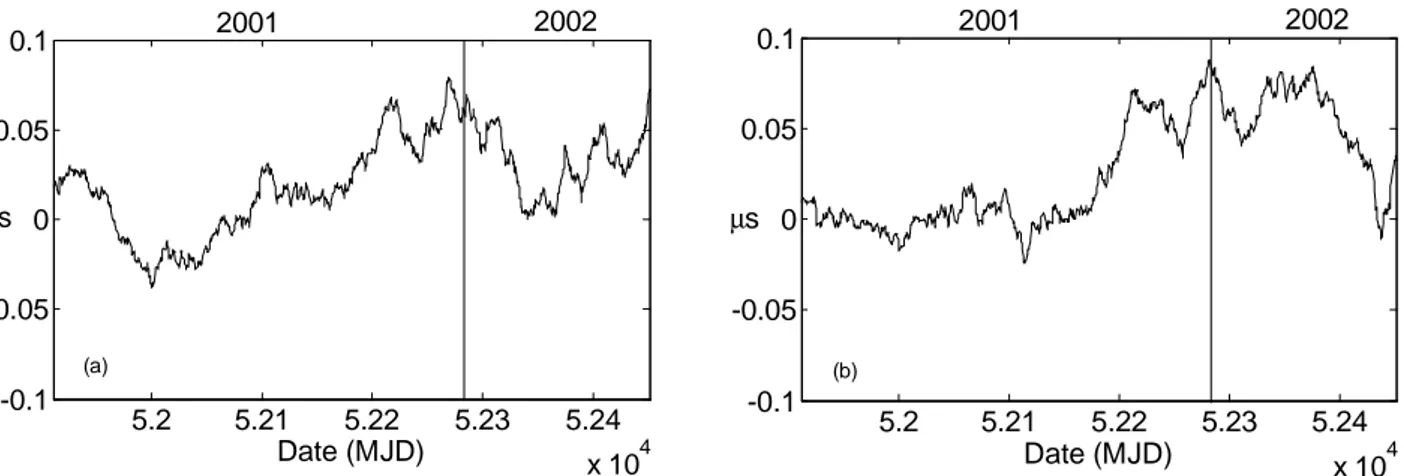
(IEN) “G. Ferraris” in Turin, Italy. The experimental data were collected every 12 hours from January 2001 to July 2002 by measuring the difference between the Italian Universal Coordinate Time UTC(IEN) and the time values provided by Cs1 and Cs3. The time deviations associated with Cs1 and Cs3 as a

func-tion of the Modified Julian Date (MJD)1, are shown in Fig. 1(a) and Fig. 1(b), respectively. In this figure, the linear systematic drift affecting the experimental data has been estimated and compensated [8]. In fact, when the analysis of the clock behavior is focused only on the random part of the error pattern, it is possible to achieve a simpler and more objective comparison between the calibration intervals obtained using the model and those calculated iteratively by means of the Simple Response Method (SRM).

A. Optimal calibration intervals estimated using the first crossing time probability

A statistical analysis of the noise affecting time measurements was performed by means of the Allan variance [9]. In fact, this statistical tool enables both the identification of the dominant noise corrupting the experimental data as well as an estimation of the noise power. From this analysis, it results that the random phase errors of the atomic clocks Cs1 and Cs3 can be satisfactorily modelled by a Wiener process

with drift. According to its definition [10], the probability of finding a moving particle in the position c at

1

MJD is an officially recognized, unambiguous dating system that, using only five digits, allows a continuous day counting starting from hour 0 of November 17, 1858 [7].

the time t is described by a normal probability density function p(·;t) with mean µt and variance σ2t, where µ and σ are referred to as the drift and diffusion coefficients, respectively. Under this hypothesis, the survival probability

P

( )

t

k2>0) can be calculated as follows [10]:

( )

( )

(

(

)

)

(

(

)

)

∫ ∑

∫

where

p

event. Observe that, in the case considered, the survival probability coincides with the EOP reliability and, consequently, it provides an estimate of the period of time during which an atomic clock can operate correctly without exceeding the given tolerance thresholds k1 and –k2. The parameters µ and σ can be

es-timated by running the noise analysis on the available time measures. Particularly, the coefficient µ can be set equal to 0 because the linear systematic drift of both clocks has been subtracted from the original data. Conversely, the diffusion coefficient σ employed in (1) is directly related to the Allan variance. This has been measured in accordance with the algorithm described in [11]. The obtained values of σ are equal (1) 5.2 5.21 5.22 5.23 5.24 x 104 -0.1 -0.05 0 0.05 0.1 Date (MJD) 2001 2002 µs (b) 5.2 5.21 5.22 5.23 5.24 x 104 -0.1 -0.05 0 0.05 0.1 Date (MJD) 2001 2002 µs (a)

Figure 1. Time differences between the Italian Universal Coordinate Time UTC(IEN) and the measurements car-ried out with Cs1 (a) and Cs3 (b) respectively, as a function of the Modified Julian Date (MJD) after the

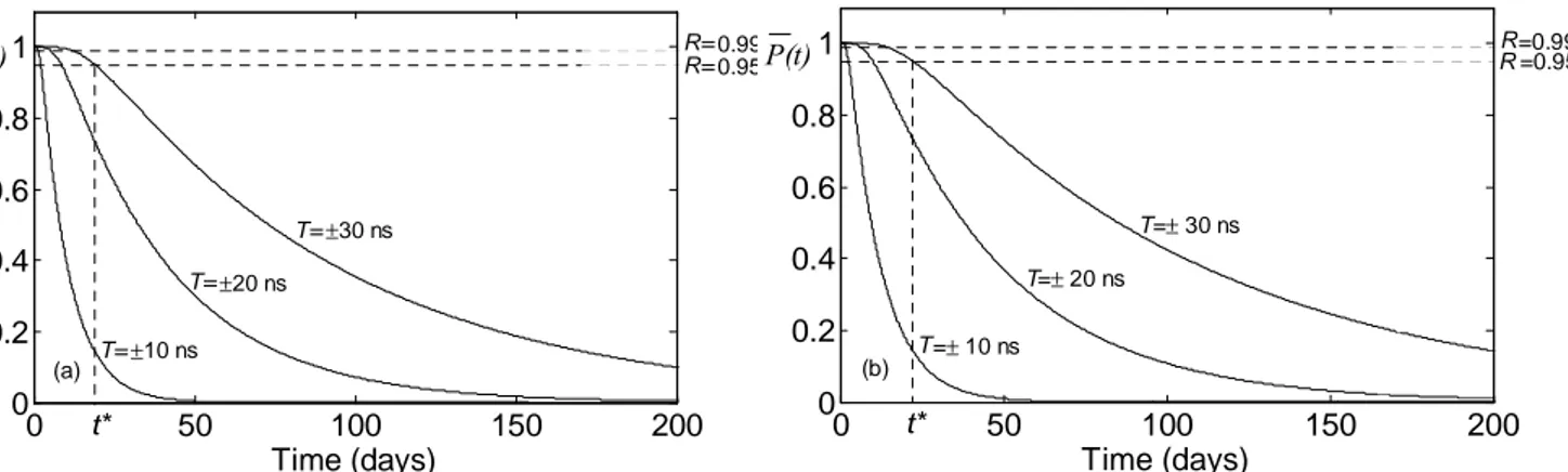
to 3.050 ns/ days for Cs1 and to 2.825 ns/ days for Cs3, respectively. Three couples of survival

prob-ability curves are shown in Fig. 2(a) for Cs1 and Fig. 2(b) for Cs3. The tolerance thresholds T=k1=−k2 used

to plot this figure are set equal to 10 ns, 20 ns and 30 ns. Clearly, the larger the tolerance interval is, the higher the probability of finding a clock in a in-conformance condition becomes. Generally speaking, the estimation of the optimal calibration interval is straightforward. After setting the survival probability equal to a given target value such as 95% or 99%, the length t* of the period of time during which clock errors are supposed to be within the chosen tolerance interval can be evaluated by reversing numerically (1). From a graphical point of view, this means simply to estimate the coordinates of the intersection point between each curve and the wished EOP reliability represented as a dashed horizontal line. As expected, the optimal calibration interval corresponding to a given target reliability is unique.

B. Optimal calibration intervals estimated using the Simple Response Method

According to the general definition of Simple Response Method (SRM), the adjustment of calibration intervals depends only on the outcome of the last calibration event: if an instrument meets the preset re-quirements, then the following calibration interval has to be increased by a factor a>0. Conversely, if the instrument is found to be out of conformance, the duration of the following interval has to be reduced by a factor 0<b<1. This behavior can be summarized as follows:

0 50 100 150 200 0 0.2 0.4 0.6 0.8 1 Time (days) P(t) (a) ±10 ns ±20 ns ±30 ns 0.99 0.95 T= T= T= R= R= t* 00 50 100 150 200 0.2 0.4 0.6 0.8 1 Time (days) (b) =± 10 ns =± 20 ns =± 30 ns P(t) =0.99 =0.95 T T T t* R R

Figure 2. Probability of finding Cs1 (a) and Cs3 (b) in a condition of metrological confirmation as a function of

time (in days). The curves shown are associated with different tolerance thresholds (i.e. ±10 ns, ±20 ns, ±30 ns). Finally, t* represents the duration of a possible optimal calibration interval when a given EOP target reliabil-ity (e.g. 95%) and a couple of tolerance thresholds (e.g. T=±30 ns) are set.

( )

( )

where In represents the duration of the n-th calibration interval, while the initial interval I0 is usually

based on an a priori risk estimate (technical intuition) of finding the instrument not calibrated at the end of the first confirmation period [1]. If Rn represents the EOP reliability of a certain instrument after the

n-th calibration event, it has been proved n-that n-the design parameters a and b of n-the SRM are related to n-the asymptotic EOP reliability R∞by the approximate expression:

(

)

Although (3) has been determined under the initial assumption that the instrument time-to-failure shows an exponential or Weibull statistical distribution, it has been verified that the same relationship holds ap-proximately even when other distributions are considered. As a result, the value of a assuring a given as-ymptotic reliability R∞can be obtained simply by reversing (3), after choosing an appropriate value of b.

In the presented application, a closed-form expression for the EOP reliability associated with Cesium atomic clocks is not available. Therefore, the EOP reliability values are estimated by computing the frac-tion of clocks whose measurement results remain inside the chosen couple of tolerance thresholds after

(2)

(3)

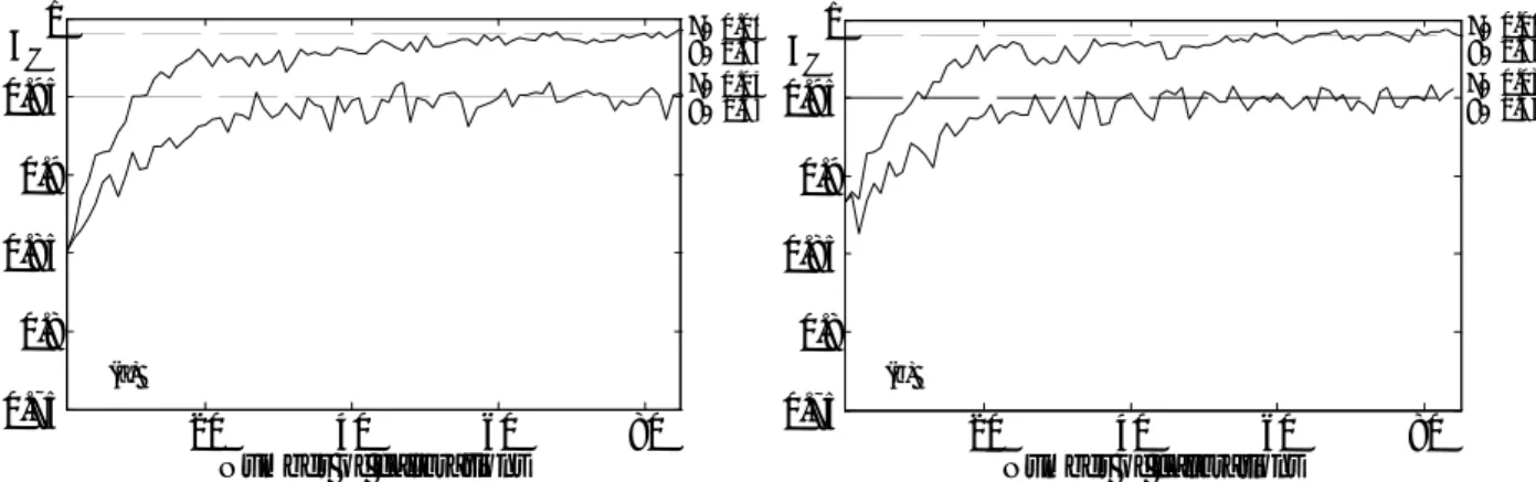
Figure 3. Reliability of the CS1 (a) and CS3(b) atomic clocks estimated using the SRM approach. The tolerance

thresholds have been set to ±10 ns, the initial interval is I0=10Ts (Ts=12 hours), while the chosen EOP target reli-abilities are equal to 99% and 95% in both cases.

20 40 60 80 0.75 0.8 0.85 0.9 0.95 1 Number of calibrations R_n (a) a= a= b= b= 0.01 0.65 0.03 0.45 20 40 60 80 0.75 0.8 0.85 0.9 0.95 1 Number of calibrations R_n (b) a= a= b= b= 0.01 0.03 0.65 0.45

Cs3, a random re-sampling mechanism has been used to improve the accuracy of the EOP reliability

esti-mators. This approach is justified by the features of the Wiener process, being the clock random error in-crements independent and identically distributed. Thus, if N represents the number of the available meas-ures, M-1 new records, with M≤NN, can be obtained by juxtaposing randomly with replacement the in-crements between adjacent clock errors calculated on the original set of data. This technique, indeed, is widely used in bootstrap algorithms to estimate the parameters of an unknown distribution of experimen-tal data whose amount is too small to allow the application of more conventional statistical techniques [12][13]. In this way, it is possible to simulate the behavior of M atomic clocks belonging to the same class. In Fig. 3(a) and in Fig. 3(b) the EOP reliabilities of a Cs1 and of a Cs3 clock family are shown for

R_∞=99% (a=0.011 and b=0.65) and R∞=95% (a=0.032 and b=0.45), respectively. In both cases the

toler-ance thresholds have been set to T=±10 ns, whereas the initial interval I0=5 days has been chosen to

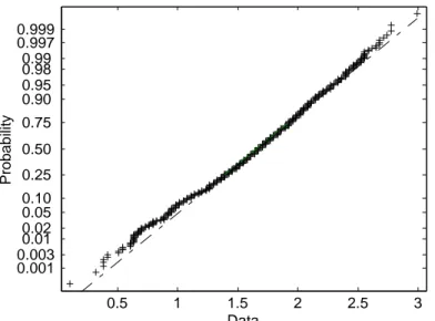
high-light the transient part of the reliability curves. Observe that, after the transient phase is finished, the clock reliability tends to settle around the asymptotic target value decided during the design stage and the dura-tion of the calibradura-tion intervals routinely shifts around the optimal value. In particular, not only is the length of the asymptotic calibration intervals calculated using (2) not constant, but also it tends to exhibit a lognormal probability distribution whose sampling mean returns a valid estimate of the optimal interval. In order to verify the assumption of lognormal distribution for the asymptotic intervals associated with Cs1, the probability plot shown in Fig. 4 has been employed. In fact, the approximate linear behavior of

such a plot supports the stated hypothesis.

III EXPERIMENTAL COMPARISON BETWEEN THE TWO TECHNIQUES

As explained in subsections II.A and II.B, for a given EOP reliability target value and for a given couple of tolerance thresholds, the application of the Wiener process model provides an unique optimal calibra-tion interval, whereas the SRM returns a distribucalibra-tion of intervals whose sampling mean can be regarded as an estimator of the optimal one. Clearly, in order to achieve significant and comparable results, the sampling mean values of the interval durations obtained with the SRM have to be calculated only when

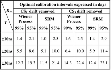
the transient phase of the instrument reliability is finished. The corresponding calibration intervals (in days) are listed in Table I after assuming two distinct target reliability values (99% and 95%) and three different couples of tolerance thresholds (T=±10 ns, T=±20 ns and T=±30 ns). The threshold selection de-pends on both the quality of the clock and the accuracy required by the application in which the clock it-self is employed. Observe that for the same values of T and R∞, the interval duration obtained using

dif-ferent methods are reasonably close to each other. In the SRM case, the standard deviations of the interval length distributions for both Cs1 and Cs3 range from about 30% to 50% of the mean values reported in

Table I, regardless of the chosen EOP target reliability value. The residual difference between each cou-ple of corresponding elements is mainly due to the inaccuracies in the model used to derive (1) and (3). These differences are particularly evident when an EOP target reliability very close to 1 is set. For in-stance, when a 99% EOP reliability is given, the SRM tends to underestimate the optimal interval. This is probably due to the fact that the SRM is employed in extreme conditions, namely using quite large values of b and very small values of a. Nevertheless, the agreement between the results achieved with both methods is extremely good.

VI. CONCLUSIONS

Figure 4. Lognormal probability plot of the asymptotic calibration intervals associated with the Cs1 atomic clock, as-suming a target reliability value equal to 95%.

0.5 1 1.5 2 2.5 3 0.001 0.003 0.01 0.02 0.05 0.10 0.25 0.50 0.75 0.90 0.95 0.98 0.99 0.997 0.999 Data P ro b a bi lity

cedure for the establishment of optimal calibration intervals of Cesium atomic clocks is described in this paper. This study is motivated by the growing importance of avoiding unnecessary calibrations without increasing the risk of making wrong measurement-based decisions. The reported results suggest interest-ing guidelines for the appropriate selection of the calibration intervals of atomic clocks. In particular, the case of atomic clock errors described by less known or less predictable stochastic processes could take advantage of the SRM procedure. Also, due to the algorithmic, general-purpose properties of the Simple Response Method, the experimental validation provided in this paper can be regarded as the starting point for the definition of widely applicable criteria aimed at managing measurement instrumentation correctly and inexpensively.

Table I. Optimal calibration intervals of the atomic clocks Cs1 and Cs3 obtained using the Wiener process model (unique value) and

the Simple Response Method (sampling mean value), respectively. In order to compare the results, the same values of EOP target reliability (99% and 95%) and tolerance thresholds (T=±10 ns, T=±20 ns and T=±30 ns) have been employed.

Optimal calibration intervals expressed in days CS1 drift removed CS3 drift removed Wiener Process SRM Wiener Process SRM 99% 95% 99% 95% 99% 95% 99% 95% ±±±±10ns 1.4 2.1 1.0 2.5 1.6 2.5 1.4 2.9 ±±±±20ns 5.5 8.6 5.1 10.0 6.4 10.0 5.9 11.4 ±±±±30ns 12.3 19.3 11.5 21.4 14.3 22.4 12.4 23.1 REFERENCES

[1] ISO 10012:2003, Measurement management systems - Requirements for measurement processes and measuring equipment.

[2] OIML Organisation International de Metrologie Legal: “Conseils pour la détermination des interval-les de réétallonage des équipments de mesure utilisés dans le laboratoires d'essais,” DI 10, 1984. [3] NCSL, Establishment and Adjustment of Calibration Intervals, Recommended Practice RP-1, Jan.

1996.

R_∞∞∞∞

[4] D. Wyatt, H. Castrup, “Managing Calibration Intervals,” Proc. NCSL Workshop & Symposium, Al-buquerque, NM, USA, Aug. 1991.

[5] A. Bobbio, P. Tavella, A. Montefusco, S. Costamagna, “Monitoring the calibration condition of a measuring instrument by a stochastic shock model,” IEEE Trans. Instr. Meas., Vol. 46, No. 4, pp. 747-751, Aug. 1997.

[6] L. di Piro, E. Perone, P. Tavella, “Random walk and first crossing time: applications in metrology,” Proc 12th European Frequency and Time Forum, Warsaw, Poland, Mar. 1998.

[7] CCIR Recommendation 457-1, Use of the Modified Julian Date by the Standard Frequency and the Time Signal Services, CCIR Green Book, vol. VII, 1990.

[8] ENV 13005:1999, Guide to the Expression of Uncertainty in Measurement.

[9] David W. Allan, “Time and Frequency (Time-Domain) Characterization, Estimation, and Prediction of Precision Clocks and Oscillators,” IEEE Transactions on Ultrasonics, Ferroelectrics, and

Fre-quency Control, vol. UFFC-34, No. 6, pp. 647-654, Nov. 1987.

[10] D. R. Cox, M. D. Miller, The Theory of stochastic processes, Science Paperbacks, Chapman and Hall, London, 1965.

[11] J.W. Chaffee, “Relating the Allan Variance to the Diffusion Coefficients of a Linear Stochastic Dif-ferential Equation Model for Precision Oscillators,” IEEE Trans. Ultras. Ferroel. Freq. Control, vol. UFF C-34, no.6, pp.655-658, Nov 1987.

[12] J. Shao, D. Tu, The Jackknife and Bootstrap, Springer-Verlag, New York, 1995.

[13] A. M. Zoubir, B. Boashash, “The Bootstrap and its Application in Signal Processing,” IEEE Signal