1
PhD Thesis in
Earth Sciences, Environment and Resources
XXXI° cycle
MACROEVOLUTIONARY ANALYSIS OF PRIMATES WITH
SPECIAL REFERENCE TO THE GENUS HOMO
Tutor:
Prof. Pasquale Raia
Coordinator:
Prof. Maurizio Fedi
Candidate:
Marina Melchionna
Matr. DR992405
2
Table of contents
Abstract ... 3
Introduction ... 5
Primates origins and diversification ... 5
Human evolution and clade diversification ... 10
Virtual Anthropology ... 16
The aim of the research ... 18
Macroevolutionary trends of brain size in primates ... 22
Unexpectedly rapid evolution of mandibular shape in hominins ... 37
Reproducing the internal and external anatomy of fossil bones: Two new automatic digital tools ... 52
A new tool for digital alignment in Virtual Anthropology ... 64
Fragmentation of Neanderthals' pre-extinction distribution by climate change ... 80
The well-behaved killer. Eurasian late Pleistocene Humans were significantly associated with living megafauna only ... 97
References ... 115
Supplementary Information for: Macroevolutionary trends of brain size in primates ... 135
Supplementary Information for: Unexpectedly rapid evolution of mandibular shape in hominins ... 143
Supplementary Information for: Reproducing the internal and external anatomy of fossil bones ... 159
Supplementary Information for: A new tool for digital alignment in Virtual Anthropology ... 165
Supplementary Information for: Fragmentation of Neanderthals' pre-extinction distribution by climate change ... 182
Supplementary Information for: The well-behaved killer. Eurasian late Pleistocene Humans were significantly associated with living megafauna only ... 207
3
Abstract
The present thesis focusses on fossil Primates, their ecological characterization, morphological evolution and diversification, and an array of new tools to study their anatomical features. The text is divided in three different parts, presenting a collection of either published or submitted manuscripts. The first part regards the morphological adaptation and diversification of Primates. The inaugural paper (“Macroevolutionary trends of brain size in primates”, Melchionna et al., under review) deals with the identification and the analysis of macroevolutionary trends in brain size evolution in Primates. We applied Phylogenetic Ridge Regression (RRphylo) to found possible shifts in morphological rates and their temporal trend. Furthermore, we computed diversification rates (DR). We found a significant increase in encephalization quotient (EQ) rates in the hominins group with an overall increase in EQ values. We found a significant correlation between DR and both EQ rates EQ values. There is also a linear relationship between speciation and extinction rates. Eventually, we found an increase in speciation rates and a reduction in extinction rates with an increase in EQ values. The second paper (“Unexpectedly rapid evolution of mandibular shape in hominins”; Raia et al., 2018) is about the evolution of mandibular shape from ancient primates to the genus Homo. We used the Geometric Mophometrics and the Phylogenetic Ridge Regression to compute evolutionary rates in mandibular morphology. We found that mandible shape evolution in hominins is exceptionally rapid as compared to any other primate clade.
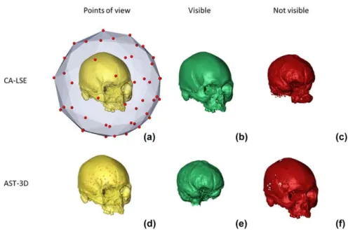
In the second part of the thesis I introduce new advances in the field of the Virtual Anthropology. The first is a new protocol to obtain three-dimensional reconstruction of inner and outer surfaces of fossil specimens (“Reproducing the internal and external anatomy of fossil bones: Two new automatic digital tools”; Profico et al., 2018). By using the R software platform, we developed two automatic tools to reproduce the internal and external structures of bony elements. The first method, Computer‐Aided Laser Scanner Emulator (CA‐LSE), provides the reconstruction of the external portions of a 3D mesh by simulating the action of a laser scanner. The second method, Automatic Segmentation Tool for 3D
4
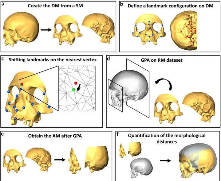
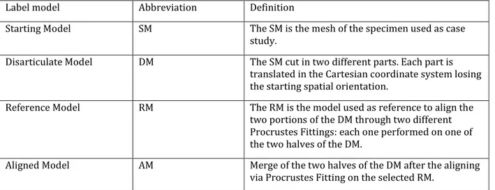
objects (AST‐3D), performs the digital reconstruction of anatomical cavities. Both methods are embedded in the packages “Arothron” (Profico et al., 2018) and "Morpho" (Schlager, 2017).The second protocol presented in this section is about the reconstruction of the original shape of fossil bones damaged and deformed by taphonomical processes (“A new tool for digital alignment in Virtual Anthropology”; Profico et al., 2018). We developed a new, semi-automatic alignment R software, Digital Tool for Alignment (DTA). This tool uses the shape information contained in a reference sample to find the best alignment solution for the disarticulated regions.
The third part of the thesis focusses on Homo, and in particularl on the relationship between Homo neanerthalesis and Homo sapiens. The first paper of this section is about the status of the Neanderthal niche fragmentation toward their demise (“Fragmentation of Neanderthals' pre-extinction distribution by climate change”; Melchionna et al., 2018). By using Species Distribution Models, and a habitat fragmentation analysis, we reconstructed the ecological niche of both human species. We found Homo sapiens had greater ecological plasticity over Neanderthals, which probably allowed this species to better react to climatic worsening at 44 and then at 40 ka. However, Neanderthals potential habitat appears to be very reduced and fragmented during the last phase of their occupation.
The second paper of this last section regards the role of Homo sapiens in the Late Pleistocene megafauna extinction (“The well-behaved killer: Late Pleistocene humans in Eurasia were significantly associated with living megafauna only”; Carotenuto et al., 2018). Starting from a rich faunal and archaeological database, and by using SDMs, we obtained megafauna and humans occurrence probability maps over the last 40 ka in Eurasia. Then, we divided species in ecological groups (i.e., body size and feeding category combined). We evaluated their geographical overlap to human range and the species suitability in the core area of Homo sapiens. The results indicated that the extinct megafauna was rare within humans' range and Palaeolithic hunters had stronger association to extant rather than extinct herbivorous species.
5
Introduction
Primates origins and diversification
One of the most intriguing question in studying the diversification of mammals, is where we humans come from. In this perspective, to study the Primate evolution is by definition the starting point. Mammalian species are known since the Mesozoic, but Primates made their appearance only between the Cretaceous and the Palaeocene periods (66 Ma). Relaxed molecular clock analyses of divergence times (Drummond et al., 2006) suggest that living Primates shared a common ancestor at 71–63 Ma (Springer et al., 2012), confirming the palaeontological data. The transition between Mesozoic and Cenozoic was marked by an intense geological change in continental organization and orogenetic processes, as best testified by the formation of the American Rocky Mountains and Andes. North America and Europe were closer than today and connected by intermittent land bridges. Africa and Europe were still separated by the Tethys Sea with no possibility of faunal migration. India had not collided with the mainland and the formation of the Himalayan mountain range had not started yet.
Traces of Primates origins can be found during the Cretaceous-Palaeocene transition. Among mammals, it has been proved that flying lemurs (Dermoptera) and tree shrew (Scadentia) can be the closest relative groups to primate and some shared adaptation could have been fundamental in their diversification and evolution (Fleagle, 2013).
Plesiadapiformes were long recognized as the first primates to appear on Earth, between the Palaeocene and the Eocene epochs (around 55 Ma). However, there is a vivid debate on the phylogenetic relationships among Plesiadapiformes, Primates and other Euarchontans (Silcox, 2007). Today, Plesiadapiformes are commonly identified as the stem group of Euriprimates (Bloch et al., 2007). They were well diffused in North America and Eurasia during the Palaeocene and the Eocene periods with almost 120 different species. They were largely diversified, both in terms of body size and dental adaptation, and represented a sizeable share of the Palaeocene mammal fauna. Plesiadapiformes were characterized by the very long snout, a flat skull with a small brain, and did not present a post-orbital
6
bar, which is one of the most important features of the Euriprimates. Their demise is probably linked to competition with other mammals or climate stated to change (Fleagle, 2013).Euriprimates diversified during the early Eocene, around 55 million years ago (Smith et al., 2006). The most remarkable climatic event at that time was a period of high temperatures, known as Paleocene-Eocene Thermal Maximum (PETM). This epoch was characterized by a marked change in North American and European faunas, where archaic types of mammals were replaced by some modern lineages. During this epoch, North America and Europe were still connected at high latitudes but became more distant through time. During this period there wasn’t polar ice, due to the warm climate conditions. Both paleogeography and paleoclimate contributed to this faunal change and to the rise and to the diversification of Primates. Moreover, today the geographical distribution of non-human primates is tropical and pan-equatorial, from around 40°S to 40°N latitude. During the Eocene the geographic range of primates extended to about 60°N latitude (Gingerich, 2012).
The first primates were markedly different from the Plesiadapiforms, with a shorter snout, smaller infraorbital foramen and the postorbital bar. They also had larger rounded brain cases and a postcranial anatomy well suited for leaping. Their digits had nails, rather than claws and they also had opposable hallux. Vision became more important over other senses due to the arboreal life and the necessity to leap between branches.
The first primates are divided in two different groups: omomyids (Eocene) and adapiforms (Eocene-Late Miocene). The first recognizable genera of both groups are Donrussellia, Cantius and Teilhardina. The appearance of these early primates was thought to be simultaneous in North America and Europe (Genus Teilhardina; Smith et al. 2006). This is not surprising, considering the geographical and climatic homogeneity in the northern hemisphere. However, the presence of Early Eocene adapiformes in Mongolia (Altanius orlovi) and Morocco (Altiatlasius koulchii) make the interpretation of Primate evolution more difficult. Moreover, new adapiforms findings in Egypt continue to add pieces to this unsolved puzzle (Seiffert et al., 2018). About similarities with the extant Primates, both adapiformes and omomyids were attributed to the extant Strepsirrhines (lemurs, galago, pottos and lorises), due to their post-orbital bar and no post-orbital closure, opposable thumbs, nails, a grooming claw, and
7
forward-facing eyes. However, today the adapiformes are closely linked with Strepsirhines, while omomyids are thought to resemble to the extant tarsiers because of the presence of large eyes and several similarities in cranial and post-cranial characteristics. During the Middle Eocene there were also primates attributable to the same families within the tarsiers. Because of these similarities, today omomyids are classified as a stem group of Haplorrhines (Rosenberger et al., 2011). However, there is not a general consensus about the phylogenetic relationship, the geographical origins, and the ancestor of the modern primate lineages, as different sources lead to different explanations.The Oligocene (34-23 Ma) was a very important epoch in primate evolution. During this epoch, the continental disposition started to look like the actual mainland shape. India had joined the Asian mainland, the Thetys Seaway was closed off and both Australia and South America were separated from Antarctica. The Oligocene was characterized by cooler and drier climate condition. A dramatic decrease in the CO2 levels in the atmosphere trigged a decrease in global temperatures and the formation of an ice-sheet at the south pole (Galeotti et al., 2016). This ice-sheet formation could have originated the Antarctic Circumpolar Current (ACC, Goldner et al., 2016) causing a severe decrease in sea levels. Due to these climate and geographical changes, there was a marked mammal faunal turn-over, including primate groups. There was the vanishing of the ancient groups as adapiformes and omomyids but, at the same time, Primates colonized tropical and subtropical biomes in both the New and the Old World (Harcourt et al. 2006; Poux et al. 2006; Schrago 2007). At the same time, anthropoids became dominant in Africa.
One of the richest fossiliferous deposits during the Oligocene comes from the Fayum Depression in Egypt. Evidences from sediment analyses show that the Fayum region was wet and warm at the time, with probable seasonality and mangrove-like plants (Fleagle, 2013). The stratigraphic sequence of the Fayum formation is rich of early anthropoid genera (Quatrania, Oligopithecus, Propliopithecus, Parapithecus, Aegyptopithecus). The Early Oligocene anthropoids were small to medium sized, they had teeth that indicate a frugivore diet, and seem to have been arboreal quadrupeds and leapers. Early anthropoid remains were also found in Asia (i.e. Eosimiids) ad some authors recognized them as basal members of the anthropoid clade (Beard and Wang, 2004).
8
The Late Oligocene is also characterized by the earliest occurrences of platyrrhines (New World Monkey) in the fossil record of South America. One of the major questions about the platyrrhine evolution is about how they arrived in South America. South America was an isolated continent, since the Eocene it begun to get further away from Africa and the connection between North and South America did not form until the Late Miocene. Evidence indicates that the first plathyrrines were anthropoids, more than prosimians (Fleagle, 2013). As there isn’t any evidence of anthropoids in North America, the dispersal across the South Atlantic from Africa seems to be the most reasonable explanation but the debate is still open.During the Miocene global temperature started to increase again. The Miocene warm climatic optimum lead to a peak in primates’ taxonomic diversity and to their colonization of tropical and subtropical biomes in both the New and the Old World (Springer et al., 2012). From the Late Oligocene to the Middle Miocene there was an extensive radiation of the ape-like catarrhines (Fleagle, 2013; Shearer et al., 2015; Arbour and Santana, 2017) and the formation of two different lineages. The first originated the living Cercopithecoids, the latter the Hominoidea.
During the Late Miocene, Hominoidea evolved following three different lineages. The first originated the living gibbons (Hylobates), in a tropical forested environment in Asia. They developed brachiation as their main arboreal locomotion system and a dentition specialized on soft fruits. The second lineage lead to oraguntans (Pongine). Their ancestors developed in a more open environment as compared to hylobatids. The third lineage is the one including Homininae.
Living Primates (around 300 species) belong to either Strepsirhine or Haplorhine. Malagasy lemurs, galagos and lorises fall into the strepsirhini clade, whereas haplorhini include tarsiers and anthropoids (monkeys, apes and humans). Primates represent a very diversified group of mammals, and even the extinct species testify a great diversity in morphological and ecological characteristics. About body size, the first primates were very tiny yet during their evolution, Primates reached huge body masses, as for Gigantopithecus blacki (Pleistocene, China, around 300 kg). Also, extant primates show a wide range in body masses, ranging in body size from 30 g in Berthe’s mouse lemur (Microcebus berthae) to 200 kg in male gorilla. Primates also show a variety of dietary adaptation. There are primates
well-9
adapted to feed on soft fruit (Macaca, Papio, Saguinus, Hylobates), while others are mostly folivore (Alouatta). Other primates can feed on trees exudates, larvae, flowers, nectar, and bark. There are also some species adapted to feed on hard food (Cacajao). Primates that live in habitats with a marked seasonality are further able to change they diet based on food availability, switching from flesh fruits during the rainy season, to hard seeds or mature leaves during the dry season (Fleagle, 2013; Tang et al., 2016).Primates stands out among mammals for their large brain volumes as compared to their body mass. The evolution of primate brain has always received great attention because of their peculiar cognitive abilities. The outstanding degree of encephalization in primates and its influence on physiological, ecological and social performance has been vividly discussed (Gould, 1975; Deacon, 1990; Dumbar et al., 2017). A very popular explanation for this increase in brain size in Primates is Aiello and Wheeler’s Expensive Tissue Hypothesis (Aiello and Wheeler, 1995). This hypothesis suggests that the metabolic requirements of large brains relative to body size are offset by a corresponding reduction in terms of gut tissue. Gut is in fact a costly organ and in Primates appears to be reduced, as compared with the overall body size. Natural selection favours large brains, but this comes at the cost of forcing high-quality diets, because the brain tissue is one order of magnitude costlier than any other tissue in the mammalian body (Isler and Schaik, 2009). As such, only calories-rich food, easy to digest also by a small gut, can afford maintaining a particularly large brain.
Different views relate selection for increased brain size to diet (DeCasien et al., 2017), home range size and activity period (Powell et al., 2017) and terrestriality and dexterity (Heldstab et al., 2016). There is strong evidence that relative brain size correlates to cognitive performance (Deaner et al., 2007; Sol et al., 2015; MacLean et al., 2012). The cognitive demands imposed by sociality are thus commonly expected to produce selection for brain expansion. This hypothesis is known as the Social Brain Hypothesis (SBH; Kudo and Dunbar, 2001; Dunbar, 2009). According to this idea, there is a strong correlation between the neocortex size in Primates and the social group size, since a large brain could bring benefits in terms of social skills, which is relevant to species living in bonded groups as it permits increased cognitive skills and behavioural plasticity. This hypothesis was implemented by many works
10
which are focused on the relationship between relative brain size, group size and mating system (Schillaci, 2006). However, patterns in brain size evolution are not always clear and even contradictory. The debate on ecological or social driven evolution of brain in Primates and humans remains open and strongly discussed (Street et al., 2017; González-Forero and Gardner, 2018).Human evolution and clade diversification
During 1849, at Forbe’s Quarry (Gibraltar) the first fossil hominid skull ever was found. Today that skull is known as Gibraltar 1 and is attributed to Homo neanderthalensis. However, at that time, the scientific community was far from recognize it as a species linked with the human lineage. The discovery of the notorious skullcap (Neanderthal 1) from the Feldhofer Grotto (Germany) in 1856 didn’t changed this view. Fossils that belong to our lineage were considered "man of low degree of civilization" (as the same Huxley wrote) or ill individuals. This point of view didn’t change for all 19th and 20th centuries. Despite this sceptical view about human origins, more and more human fossils came to light, both in Europe and Asia. In 1891, at Trinil, Java (Indonesia), Eugene Dubois found the calvaria that he attributed to a new species, Pithecantropus erectus (today know as Homo erectus). In 1907 at Mauer, in Germany, a single jaw was found and represent the specimen type of Homo heidelbergensis (Schoetensack, 1908). Discoveries of remains that claims at a more intricate human evolution history than previously thought continued to increase. The European scientific community started to feel an historical urgency to re-establish the integrity of the origin of the human species, especially in contrast with the rising idea of an African origin of Homo sapiens. During the first half of the 20th century, the widespread nationalism and racism brought to one of the most (in)famous archaeological fakes in history, the Piltdown man. The “discovery” of the Piltdown Man came in 1912. It consists in a composite skull with an admixture of pieces from human skull and an orangutan jaw. Scientists were searching for the ‘missing link’ between apes and humans, and the fact that this almost human ancestor was found in England didn’t left room for further investigations. The Piltdown Man validity remained unquestioned until 1957, when further
11
analyses on the remains proved it was a fake. Sadly, the Piltdown Man hoax caused a delay in human evolution investigation. Raymond Dart discovery of the Taung child (Australopithecus afarensis; Dart, 1925) and its linking with human lineage evolution were strongly criticised by the British scientific community, that continued to deny the affinity with the human ascent. After the Piltdown Man retraction, all hominid remains were re-examined, and an African origin of our species was finally established. The main question at this point is: where and when can the starting point of human origin be placed?The separation of the lineages leading to the living African apes on the one hand and to humans on the other took place between 10 million and 5 Ma, during the Late Miocene (Fleagle, 2013). At that time, dramatic climatic and biotic turnovers took place. Tectonic events like the uplift of the Himalayas and the Tibetan Plateau, the closure of the Atlantic-Indian seaway throughout the Mediterranean, and the desiccation of Paratethys and Mediterranean seas (Agustì, 2007) are claimed to be related with this turnover. Moreover, the new geographical organization of lands brought to a different circulation system with the formation of a permanent Antarctic ice-sheet, the instauration of a monsonic regime and a general increase in seasonality (Zachos et al., 2001). The African continent maintained the woodland vegetation at West, while at East the vegetation became more open with an increase in bushes and C4 grassland.
These geographical and ecological changes are claimed to be the major explanation of the separation between African apes and humans. The first remain that can be undoubtedly ascribed to our lineage is Sahelanthropus tchadensis (6-7 Ma) in the site of Torros-Menalla, in western Djurab Desert of Chad, Central Africa (Brunet et al., 2002). It consists in a single partially deformed skull. Even if no post-cranial remains were found, the foramen magnum position clearly indicates that S. tchadensis was bipedal. Other early evidence of bipedalism is to be found in Orrorin tugenensis and Ardipithecus (6-5 Ma; Richmond and Jungers, 2008). There are different theories about the origin of bipedalism. Whatever the truth, bipedalism represents an unquestionable evolutive advantage. Being able to stand upright frees the hands from locomotor duties and allows to carry things and use tools. Moreover, with the
12
progressive opening of the vegetation, bipedal position allows to see over the tall grass as a defence from predators.From 4 to 2 Ma two different hominin genera were present in Central, East and South Africa, Australopithecus and Paranthropus. Australopithecus genus was at base of evolution of both Paranthropus and Homo. The major characteristic of Australopiths are a bigger brain in relation to body size, compared to the extant non-human Primates, large molars with thick enamel and a thick mandible with high ascending ramus. Australophits were able to walk in an upright position, as testified by the Laetoli footprints (3,7 Ma; Raichlen et al., 2010) and by the postcranial evidences (elongate forelimbs, flat feet, enlarge hip bones). However, Australopiths were also able to climb trees if necessary. A recent re-analysis of Lucy (Australopithecus afarensis, Hadar, Ethiopia, 3,18 Ma) one of the best-known samples of Australopithecus, showed injuries resulting from a fall, probably out of a tall tree (Kappelman et al., 2016).
Paranthropus represent a widespread genus in both East and South Africa. Also known as the robust australopiths, they have larger molars and premolars combined with relatively smaller canines and incisors (Fleagle, 2013). Their powerful jaws were claimed to be useful for feed on a variety of hard seeds. Recent evidences on dental isotopes (Cerling et al., 2011) suggest that, except for Paranthropus boisei, both Australopiths and Paranthrops had a C3-based diet. This difference can represent an adaptive divergence between the eastern and southern African Paranthropus populations. Contrary to previously thought, Australipiths and Paranthropus species were tools users. Both anatomical (Skinner et al., 2015) and archeological (Semaw, 2000; McPherron et al., 2010; Harmand et al., 2015) evidences support this view.
In 1960, at Olduvai Gorge (Tanzania) Jonathan and Mary Leakey found OH7, a fragment parts of the lower mandible. This fossil became the type specimen of a new species, Homo habilis. The main differences between early Homo and Australopithecus are the small molars and premolars, larger brains a more human-like limb proportion with longer legs, a narrowed thorax and straight phalanges.
Homo habilis appeared in East Africa around 2.5 Ma. The best-known sites of H. habilis are Olduvai Gorge (Tanzania) and Turkana Basin (Ethiopia). These early hominins were recognized to be
13
the producer of the ancient and well-definable industry, the Oldowan. The Oldowan industry consist in choppers and scrapers which were probably used for butchering small animals and crushing the largest bones to reach the bone-marrow.In 1984, at Lake Turkana (Kenya) the notorious Turkana boy (KNM-WT 15000; around 1.6 Ma) was found an almost complete skeleton of Homo erectus. The Turkana boy was an adolescent at the time of death. He was tall and the limb proportion appears to be similar to Homo sapiens. Homo erectus is associated with the Acheulean industries, which consist in hand-axes and bifacial tools. They had a mostly carnivorous diet and they were probably scavengers. The meat consumption was so marked that some authors hypnotized a large consumption of liver which could have caused hypervitaminosis A in Homo erectus (Walker et al., 1982). Homo erectus was the first human species that came out from Africa (Carotenuto et al., 2016). Moreover, the findings at Dmanisi (Georgia) prove that this earlier dispersal happened before than 1.75 Ma, which is the estimated age for the Dmanisi site (Vekua et al., 2002; Lordkipanidze et al., 2013). Archaeological evidences show that Homo erectus was present in Asia from 1.8 to 0.5 Ma and in Europe from 1.4 to 0.9 Ma (Joordens et al., 2005; Carotenuto et al., 2016). Because of the wide distribution of this species, there are several anatomical differences between the African and the Eurasiatic type. For that reason, some authors prefer a different nomenclature for the African (Homo ergaster) and the Eurasiatic remains (Homo erectus).
Homo heidelbergensis (700-130 ka) is an archaic hominid claimed to be the last common ancestor of Homo sapiens and Homo neanderthalensis. Fossils of H. heidelbergensis are known from South Africa (Broken Hill, Berg Aukas), East Africa (Bodo), Italy (Ceprano), Germany (Heidelberg) Greece (Petralona) and possibly China (Dali) (Fleagle, 2013). Cranial remains associated to Homo heidelbergensis show a mean brain size of 1,250 cm3, a low and flattened frontal bone, a large and continuous supraorbital torus. Postcranial remains (Roberts et al., 1994) indicates that they were strong and tall. The status of Homo heidelbergensis is crontroversal and a debate on the attribution of his remains is still on (Mounier et al., 2009; Stringer, 2012; Manzi, 2016).
It is now accepted that the origin of Homo sapiens can be found in Africa, from the previously described Homo heidelbergensis. The oldest evidences of an African evolution of our species comes from
14
a mandible found at Jebel Irhoud, in Morocco (Hublin et al., 2017), dated around 300 ka. Other evidences of such evolution are from the Kibish Formation in Ethiopia (Omo 1 and Omo 2, 200 ka; Shea et al., 2007) and Herto, in the Middle Awash region of Ethiopia (White et al., 2003). Our species is well-distinguished from other members of the genus Homo. Some of the main characteristics are the small teeth with a vertical mandibular ramus, the chin, a reduced brow ridge and a vertical forehead with a well-developed frontal cortex in comparison with the whole brain size. Archaic homo sapiens ventured out twice in their evolutionary history. The human remains at Skhul and Qafzeh at Mount Carmel, in Israel (120-90 ka, Grün et al., 2005) were retained the evidence of the first Out of Africa event. A recent discovery of archaic human remains at Misliya Cave (Israel; Hershkovitz et al., 2018) suggested that our species had already left Africa at 180 ka. However, there is no evidence of a stable human colonization of Europe until 40 ka (Mellars, 2006; Benazzi et al., 2015). Scientists usually refer to these modern Homo sapiens as anatomically modern humans (AMHs). At the end of the Pleistocene human populations begun their spread throughout the globe that would lead to a tenfold increase in population in over thousands of years (Mellars e French, 2011) and then to the actual distribution around the globe (Timmerman and Freidrich, 2016).During the Late Pleistocene there was another species in Eurasia, Homo neanderthalensis, which stands alongside AMHs. The oldest evidence of a Neanderthal population was found at Zuttiyeh (Israel), with an age around 200.000 years ago, Tabun (Mount Carmel, Israel) around 150,000 years (Grun et al., 1991) and Altamura (Italy) at around 150,000 years (Lari et al., 2015). Neanderthals present unique morphological characteristics that make them very different from our species. They had a large nasal cavity, a large brow ridge and in general their skullcap is more elongated then Homo sapiens cranium. The short limb proportions suggesting a limited stature (Helmuth, 1998) with males estimated at 165.9 cm tall and 77.6 kg in body mass (Ruff et al., 1997). Moreover, Neanderthals had a wide chests and large lung volume (Franciscus & Churchill, 2002; Macias & Churchill, 2015). These features were long thought to represent an adaption to cold, in accordance with well-known ecogeographic Bergmann’s and Allen’s rules. Higham and colleagues (2014) statistically placed the extinction of Homo neanderthalensis around 40 ka, almost in coincidence with Heinrich Event 4 (HE4). This event consists in a sudden and global
15
shift towards colder temperatures (Van Meerbeeck et al., 2009). It has been demonstrated that Neanderthal populations experienced major demographic contractions during the HE4 cold event in Northern Iberia and Southern France (d’Errico & Goñi 2003; Sepulchre et al., 2007). Contrary to the previous assumptions, this evidence shows that Neanderthals were not well-adapted to cold climate conditions. There are different studies that seem to support this hypothesis (Finlayson & Giles, 2000; Stewart, 2004; 2007; Bradtmöller et al., 2012). The late contraction of H. neanderthalensis range to southern Europe coincides with the spread of AMHs, suggesting a possible instance for competitive exclusion between the two (Banks et al., 2008; Mellars &; French, 2011). Negative interactions between Neanderthals and AMHs are often viewed as the potential drivers of H. neanderthalensis extinction, as an alternative to climate change hypothesis, or a combination of the two causes (Rey-Rodríguez et al., 2016).The relationship between AMHs and Neanderthals could have been more complicate than expected. It is now demonstrated that Neanderthals share genetic variants with present-day humans in Eurasia, but not with sub-Saharan Africans, suggesting that gene flow from Neanderthals into the ancestors of non-Africans occurred before the divergence of Eurasian groups from each other (Green et al., 2010). Another evidence of a genetic admixture between Neanderthals and modern humans come from Peştera cu Oase (34-36 ka, Trinkaus et al., 2003) and Ust' Ishim (45 ka, Fu et al., 2014) specimens, which shows a close derivation from a Neanderthal individual. Particularly, the Peştera cu Oase specimen should have had a Neanderthal ancestor as recent as four to six generations before it lived (Fu et al., 2015). It has been suggested that that Neandertal alleles may have helped modern humans adapt to non-African environments during their dispersal (Sankararaman et al., 2014). In modern humans there is the 3.3–5.8% of Neanderthals genome. In this scenario, Neanderthals could be seen as a species on the verge of extinction that was genetically assimilated into the AMH population. Traces of Neanderthals extinction can be found still today, in our genome. There are regions of millions of base pairs that are nearly devoid of Neandertal ancestry (“deserts”), implying a negative selection to remove genetic material derived from Neandertals (Kuhlwilm et al., 2016).
16
AMHs and Neanderthals were not the only Homo species in Eurasia during the Late Pleistocene. In 2008, the distal manual phalanx of the fifth digit of a hominin was excavated in Denisova Cave (Altai region, Siberia). The exceptionality of this discoveries wasn’t understood until 2010, when Krause and colleagues started to sequence the genome of that phalanx. The mtDNA showed that this specimen was from any other known hominis, but it appeared to belong to an unknown species that shares a common ancestor with AMHs and Neanderthal mtDNAs about 1.0 million years ago. Indirect dates indicate that this individual lived between 30.000 and 50.000 years ago (Reich et al., 2010), overlapping in time and space with both Neanderthals and humans. If traces of Neanderthal admixture with our genome can be found only in non-African individual, the distribution of the Denisovan genome is even more peculiar. A worldwide genome analysis showed that the high percentage of genetic admixture with Denisovans can be found in Southeast Asia and Oceania, with a 4–6% of its genetic material to the genome of present-day Melanesians (Reich et al. 2010; Vernot et al., 2016; Sankararaman et al., 2016). In this scenario, some authors identified a first split between Neanderthals and Denisovans from modern humans (550–765 ka), then a second split of Neanderthals and Denisovans to 445–473 ka (Prüfer et al., 2014). Evidences of an admixture with Neanderthals and Denisovians continues to come to light (Slon et al., 2018)Virtual Anthropology
Remains which testify our evolutionary history raise enthusiasm and a great interest in the scientific community. However, hominins fossils are rare. They are often damaged or too delicate, inaccessible in most of the cases. The use of 3D models is revolutionizing the study of the human fossil record, giving rise to the burgeoning field of “Virtual Anthropology” (Weber, 2001). By using medical technology as laser scanner, CT-scan and magnetic resonance imaging (MRI), the permanent accessibility of the virtual objects is allowed. This kind of technology gives access to new information and the possibility to study inner structures and cavities which cannot be seen otherwise.
17
For surface measurements and analysis, a laser scan technology can be useful to record the complete surface and isolating skeletal elements (Aiello et al., 1998). To study and reconstruct inner cavities, the CT-scan technology is largely used today, since the real object has been converted into a virtual specimen throughout the volume (Weber, 2001). The data acquisition is made through a computed tomography scanner (CT-scanner) which produce the complete image volume of the analysed object. The CT-scanner collects numerous cross-sectional images ("slices") from different directions. Dedicated software can reconstruct the three-dimensional image of the analysed object from the large amount of two-dimensional radiographic images. The final data can be viewed as an image in any triplet of orthogonal planes, as well as from any arbitrary view.The output of a CT scanner is a 3D data matrix, consisting of small information units, called voxels, comparable to pixels in 2D. Each voxel is labelled by three Cartesian coordinates (x, y and z). Eventually, voxels can be converted in triangular mesh by specific algorithm and software. The final 3D object is a surface mesh formed by a net of oriented triangular facets, which are individually defined by the coordinates of their vertices and by their mutual connections. The collection of vertices, coordinates, and connections defines the shape of the virtual surface in the computer language (Weber and Bookstein, 2011).
The CT-scan technology allows the application of such procedures to whichever specimen whose preservation is good enough to present quality details. The use of CT-scan consents to access inner cavity sizes and shapes, such as the ear structure (Gunz and Mitteroecker, 2013), cranial nerve organization (Ibrahim et al., 2014), the trabecular bone geometry (Chirchir et al., 2015; Ryan and Ketcham, 2002), and brain endocasts (Falk et al., 2005; Beaudet and Bruner, 2017; Diniz-Filho and Raia, 2017). CT-scan technology and 3D modelling techniques can be successfully applied for reconstructing missing or damaged part of a fossil specimen (Gunz et al., 2009; Profico et al., 2016a; Di Vincenzo et al., 2017) and restoring the bilateral symmetry of a digital mode (Schlager et al., 2018).
18
The aim of the researchThe present thesis is focussed on fossil Primates, their ecological characterization, morphological evolution and diversification, and the new tool to study their anatomical features. The thesis is divided in three different part.
The first part regards the morphological adaptation and diversification of Primates. The expansion of their relative brain size is one of the most peculiar characteristics of primate evolution, but motivations behind this trend are still vividly debated. The first paper presented here (“Macroevolutionary trends of brain size in primates”, Melchionna et al., under review) is about the identification and the analysis of macroevolutionary trends in brain size evolution in Primates. By using new comparative phylogenetic method, Phylogenetic Ridge Regression (RRphylo; Castiglione et al., 2018), we searched for possible shifts in the evolutionary rate in encephalization across the primate tree (from the stem group of Plesiadapiformes to the genus Homo). In addition, we computed the rates of taxonomic diversification and regressed them against evolutionary rates in encephalization, to see whether encephalization induced higher diversification. In the last phase of the analysis, we applied Pradel’s models (Pradel, 1996; Finarelli et al., 2016) on palaeontological data to investigate trends in speciation and extinction rates with the aim to assess their influence on diversification patterns. We found a significant increase in EQ rates in the hominins group with an overall increase in EQ values. We found a significant correlation between DR and both EQ rates EQ values. There is also a linear relationship between speciation and extinction rates. Eventually, we found an increase in speciation rates and a reduction in extinction rates with an increase in EQ values.
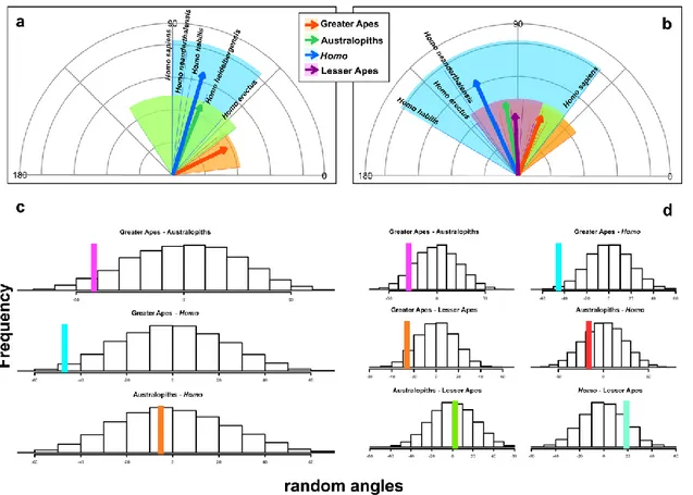
The second paper (“Unexpectedly rapid evolution of mandibular shape in hominins”; Raia et al., 2018) is about the evolution of mandibular shape from the ancient primates to the genus Homo. It’s known that diet and mandibular shape, as well as body size, are some of the main drivers of ecological diversification in fossil, as well as in living primates. Members of the hominin clade have been long noted for their short and deep mandibles, low-cusped molars, and reduced incisors and canines. These traits evolved in early members of the clade in response to changing environmental conditions of the Early
19
Pleistocene and the consequent increase in consumption of though food items. The evolutionary trend in the change of mandibular shape were thought to be weak in the genus Homo, because of the the tool use and the control of fire. To study the mandibular change in primates we used the Geometric Mophometrics (Adam et al., 2004; Klingenberg, 2010) and the Phylogenetic Ridge Regression to compute evolutionary rates in mandibular morphology. The results were unexpected. We found that mandible shape evolution in hominins is exceptionally rapid as compared to any other primate clade. We also performed a multivariate angle computation analysis to verify whether the mandibular shape trajectory in australopiths and Homo were parallel, and whether they differed from that of non-hominin apes. We found that both direction and rate of shape change (from the ape ancestor) are no different between the australopiths and Homo.In the second part of the thesis I introduce new advances in the field of the Virtual Anthropology. The first is a new protocol to obtain three-dimensional reconstruction of inner and outer surfaces of fossil specimens (“Reproducing the internal and external anatomy of fossil bones: Two new automatic digital tools”; Profico et al., 2018). Starting from the CT-scan of a fossil specimen, the traditional protocol for the acquisition of their 3D surfaces is time-consuming and it depends on the manual ability of the operator (Profico et al., 2016b; Huotilainen et al. 2014; Nicolielo et al., 2017). Also, the softwares commonly used to perform the surfaces acquisition can be very expensive and difficult to use. By using the R software, we developed two automatic tools to reproduce the internal and external structures of bony elements. The first method, Computer‐Aided Laser Scanner Emulator (CA‐LSE), provides the reconstruction of the external portions of a 3D mesh by simulating the action of a laser scanner. The second method, Automatic Segmentation Tool for 3D objects (AST‐3D), performs the digital reconstruction of anatomical cavities. Both methods are embedded in the packages “Arothron” (Profico et al., 2018) and "Morpho" (Schlager, 2017).
The second protocol presented in this section is about the reconstruction of the original shape of fossil bones damaged and deformed by taphonomical processes (“A new tool for digital alignment in Virtual Anthropology”; Profico et al., 2018). Since fossil remains are often fragmented and/or deformed by taphonomic processes, a preliminary re-alignment of their constituent parts is often necessary to
20
properly interpret their shapes. Three-dimensional imaging techniques allow substituting manual alignment with virtual protocols, which guarantee the physical preservation of the fossil specimen avoiding potential alterations of its original shape, as introduced by the manual operator. In this paper a new semi-automatic alignment R software tools, Digital Tool for Alignment (DTA), is presented. This tool uses the shape information contained in a reference sample to find the best alignment solution for the disarticulated regions.The third part of the thesis is focussed on genus Homo, particularly on Homo neanerthalesis and Homo sapiens. The first presented paper of this section is about the status of the Neanderthal niche fragmentation toward their demise (“Fragmentation of Neanderthals' pre-extinction distribution by climate change”; Melchionna et al., 2018). Neanderthals went extinct around 40 ka (Higham et al., 2014) and the role of both Late Pleistocene climate worsening and human competition were proposed as main causes of extinction. The Neanderthal demise is very complex to interpret. Neanderthals were found to have had small population size and high mortality rates (Sørensen, 2011; Bocquet-Appel and Degioanni, 2013). There are evidences of an early extinction of Northern European populations before 48 ka followed by recolonization from the Middle East, while Southern populations persisted there (Fabre et al., 2009). Furthermore, genetic evidences support this scenario, pointing out a species divided into a number of small and isolated populations (Rogers et al., 2017). By using Species Distribution Models, and a habitat fragmentation analysis, we reconstructed the Neanderthals and human ecological niche. We found Homo sapiens had greater ecological plasticity over Neanderthals, which probably allowed this species to better react to climatic worsening at 44 and then at 40 ka. However, Neanderthals potential habitat appear to be very reduced and fragmented during the last phase of their occupation.
The second publication of this section regards the role of Homo sapiens in the Late Pleistocene megafauna extinction (“The well-behaved killer: Late Pleistocene humans in Eurasia were significantly associated with living megafauna only”; Carotenuto et al., 2018). Human hunting is often depicted as the major driver of megafauna demise (‘overkill hypothesis’). However, the magnitude of the human influence is not clear and might have had different patterns in the Old and the New World. Moreover, studies on living population of hunter-gathers revealed that only a small percentage of energetic supply
21
comes from hunt (Hill and Hurtado, 2009; Hill et al., 2013). By using SDMs, we obtained megafauna and humans occurrence probability maps over the last 40 ka in Eurasia. Then, we divided species in ecological groups (i.e., body size and feeding category combined). We evaluated their geographical overlap to human range and the species suitability in the core area of Homo sapiens. Intriguingly, results showed that the extinct megafauna was rare within humans' range and Palaeolithic hunters had stronger association to extant rather than extinct herbivorous species.22
Melchionna et al. under review. Proceedings of the Royal Society B
Macroevolutionary trends of brain size in primates
Abstract
Primates are among the most successful mammalian groups. One of the most peculiar characteristics of primate evolution is the expansion of their relative brain size. The motivation behind this trend is vividly debated. Here, we assembled a phylogeny for 318 primate species, including both extant and extinct taxa, to identify macroevolutionary trends in brain size evolution by applying a new comparative phylogenetic method, Phylogenetic Ridge Regression (RRphylo). We computed the rates of taxonomic diversification and regressed them against the evolutionary rates in encephalization, to see whether encephalization associates to diversification. Our findings show a neat macroevolutionary trend for increased encephalization apply to all Primate, although hominins stand out for distinctively higher rates and phenotypes.
We found a strong association between diversification rates and degree of encephalization. A strong increase in diversification applies since the beginning of the Oligocene and seem to coincide well with the appearance of Anthropoids.
23
IntroductionPrimates are among the most successful mammalian orders. Their last common ancestor lived some 71 to 63 million years ago (Springer et al., 2012). Plesiadapiforms are the oldest known stem primates (Bloch et al., 2007). These tiny arboreal species appeared in North America around the Paleocene/Eocene boundary and spread throughout Europe and Asia afterwards. The phylogenetic relationships between the (most probably polyphyletic) Plesiadapiforms and true primates is still discussed. The oldest unquestionable crown primates belong to omomyids (Eocene), and adapiforms (Eocene-Late Miocene). During the Miocene warm climatic optimum, primates peaked in taxonomic diversity and colonized tropical and subtropical biomes in both the New and the Old World (Springer et al., 2012). Living Primates belong to either Strepsirhine or Haplorhine. Malagasy lemurs, galagoes and lorises fall into the strepsirhini clade, whereas haplorhini include tarsiers and anthropoids (monkeys, apes and humans).
The evolution of primates always received great attention because of their peculiar cognitive abilities. Primate brain expansion, both in absolute (endocranial volume, ECV) and relative (encephalization quotient, EQ) terms, is one of the main peculiarities of the group (Montgomery et al., 2016). The outstanding degree of encephalization in primates and its influence on physiological, ecological and social performance has been vividly discussed (Gould, 1975; Deacon, 1990; Dunbar and Shultz, 2017). According to the Expensive Tissue Hypothesis (Aiello and Wheeler, 1995), natural selection favours large brains, but this comes at the cost of forcing high-quality diets, because the brain tissue is one order of magnitude costlier than any other tissue in the mammalian body (Isler and van Schaik, 2009). As such, only calories-rich food can afford maintaining a particularly large brain (Mink et al., 1981; Isler and van Schaik, 2006). Different views relate selection for increased brain size to diet DeCasien et al., 2017), home range size and activity period (Powell et al., 2017), mating system (Schillaci, 2006), and terrestriality and dexterity (Heldstab et al., 2016). There is strong evidence that relative brain size correlates to cognitive performance (Sol et al., 2005; Deaner et al., 2007; MacLean et al., 2012). The cognitive demands imposed by sociality are thus commonly expected to produce selection for brain expansion (the Social Brain Hypothesis, SBH; Kudo and Dunbar, 2001; Dunbar, 2009). Although this link
24
extends to animal clades other than primates (Marino et al., 2004; Montgomery et al., 2013), SBH remains open and strongly discussed (Street et al., 2017; González-Forero and Gardner, 2018).Since brain size scales allometrically to body size (Isler et al., 2008; Grabowski et al., 2016) most studies addressing encephalization patterns uses EQ as the reference metrics. However, both brain and body sizes influence EQ, that makes it difficult to disentangle their relative selection effect on encephalization, so that ECV is often taken as the best proxy for encephalization (Deaner et al., 2007; Shultz and Dumbar, 2010).
At the macroevolutionary level, increased brain size was found to relate to diversification dynamics. Large brain size (EQ) reduces extinction risk in birds (Sol et al., 2005) and mammals (Isler and Schaik, 2009; Sol et al., 2008). Clade-level ECV patterns are associated to origination and extinction processes in hominids (Du et al., 2018), and a significant increase in EQ corresponds to a shift in diversification rate in carnivores (Finarelli an Flynn, 2009). There is substantial evidence for increases in speciation rates in Primates (Gómez and Verdú, 2012; Arbour and Santana, 2017; Herrera, 2007). Yet, it is still unknown how these relate to encephalization.
Our goal here is to identify and analyze macroevolutionary trends in brain size evolution in Primates. We assembled a large paleontological phylogeny (Raia et al., 2018) inclusive of 318 primate species we had endocranial volume (ECV) and body mass estimates for. We applied Phylogenetic Ridge Regression (RRphylo, Castiglione et al., 2018) to search for possible shifts in the evolutionary rate in encephalization across the primate tree. Then, we present an implementation of RRphylo designed to search for phenotypic evolutionary trends, which we apply to study encephalization patterns. Furthermore, we computed the rates of taxonomic diversification and regressed them against evolutionary rates in encephalization, to see whether encephalization prompted higher diversification, as often posited in the scientific literature. Eventually, we used Pradel’s models (Pradel, 1996; Finarelli and liow, 2016) applied on palaeontological data to investigate trends in speciation and extinction rates and assess their influence on diversification patterns.
25
Material and methodsData preparation
We collected from literature estimates of primate body mass and endocranial volume (ECV) (see Appendix 1). Our dataset and tree include 318 species, both extant (248) and extinct (70), ranging from Paleogene plesiadapiforms to extinct and living primates. ECV data only include direct estimations of the brain cavity volume. In keeping with Grabowski and colleagues (Grabowski et al., 2016), we computed encephalization quotients (EQ) from ECV and body mass estimates (see Appendix 1) according to the equation:
𝐸𝑄 = 𝐸𝐶𝑉
𝑒0.60 ln(𝐵𝑀)−1.402
where ECV is the endocranial volume, and BM is body size; Grabowski et al., 2016).
RRphylo
We applied a recently-implemented Phylogenetic Comparative Method (PCM) that is specifically thought to work with phylogenies including fossil species. The RRphylo method (Castiglione et al., 2018) performs phylogenetic ridge regression (Kratsch and McHardy, 2014) on tree and data in order to compute phenotypic evolutionary rates for each branch of the phylogeny. Under RRphylo, evolutionary rates are computed as regression coefficients. As such, they can be either positive or negative, indicating the direction of phenotypic change (increase or decrease). The magnitude of the rate is represented by the coefficient absolute value. RRphylo allows removing the effect of a covariate on the evolutionary rates. In the present case, the function computes rates on the residuals of either ECV or EQ regressed against body size (all data were ln-transformed before analyses).
After computing the evolutionary rates, for each variable (i.e. body mass, ECV, and EQ) we searched for rate shifts across the tree by applying the function search.shift (Castiglione et al., 2018). The latter uses randomizations to see whether specific clades have higher absolute rate values than the rest of the tree.
26
To search for temporal trends in phenotypes and rates, we applied a new RRphylo function, named search.trend. The function regresses evolutionary rates and phenotypic values (the original tip values plus the ancestral states estimated through RRphylo) against their age, and then compares the regression slopes to slopes generated by simulating data with no trend in either phenotypic mean or variance. The performance of search.trend was assessed by means of simulation experiments. It revealed to perform with low Type I and Type II error rates (see Electronic Supplementary Material). All the functions are available as part of the R package RRphylo (Raia et al., 2018b) available at https://github.com/pasraia/RRphylo.Diversification Rate (DR)
We used the DR statistic (Jetz et al., 2012) as a metric for diversification rate. DR has been shown to work well on both living and fossil phylogenies (Cooney et al., 2017; Cantalapiedra et al., 2017), and proved to be particularly well-suited to investigate the correlation between diversity and disparity dynamics (Harvey and rabosky, 2017), which was our goal here. DR is computed as the inverse of equal splits, which represent the proportion of the total evolutionary time in the phylogenetic tree attributed to each lineage (Redding and Mooers, 2006). This metric has the advantage of giving a distinct rate to each species, thus allowing a lineage-by-lineage investigation of the correlation between taxonomic and phenotypic diversification rates. We also tested the relationship between DR and endocranial volumes (ECV), and encephalization quotient (EQ) separately, looking for possible anatomical drivers of diversification.
Pradel models
Pradel models [38] belong to Jolly-Seber family of capture-mark-recapture (CMR) models. In keeping with Finarelli and Liow (Liow and Finarelli, 2014; Finarelli and Liow, 2016) we used such implementation on paleontological data in order to estimate interval-to-interval extinction, origination, diversification and sampling probabilities.
27
Survival probability (𝜑𝑖) is defined as the probability of a species surviving from the interval i to the interval i+1. Thus, the complement of this term (1-𝜑𝑖) is the probability of extinction from time i to time i+1. Seniority (γi) is the probability that a species extant at interval i was already present duringthe interval i-1. Thus, the complement of this term (1-γi) is the speciation probability from time i-1 to
time i. This parameter is related to recruitment, fi, which is the number of new species appearing at
interval i+1 divided by the number of species present at interval i. Recruitment is computed as: 𝑓𝑖 =
𝜑𝑖( 1−𝛾𝑖+1
𝛾𝑖+1 ). Growth rate (λi) is defined as the ratio between the number of species at intervals i+1 and i. It can be also computed as: 𝜆𝑖 = 𝑓𝑖+ 𝜑𝑖. Therefore, the net per capita diversification rate is:
𝑁𝑖+1−𝑁𝑖 𝑁𝑖 = 𝜆𝑖− 1. Eventually, sampling probability (pi) is the probability for a species actually extant during
interval i to be sampled in that very interval.
We divided fossil occurrences in consecutive, one million years long time bins. Then, we built two types of Pradel’s models, one based on the estimation of ‘survival and seniority’ (which fits extinction, speciation, and sampling rates) and the other on the estimation of ‘survival and population growth’ (which fits extinction, diversification, and sampling rates) through time. The application of two different models is necessary because parameters are linear functions of each other (i.e. they are defined by a family of linear equations).
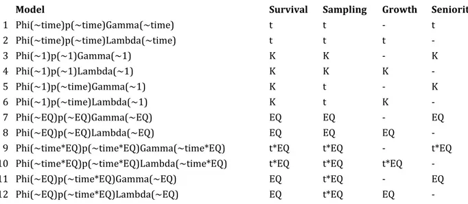
We were interested in the course of diversification metrics (speciation and extinction) over time, and how and whether they were affected by EQ. Therefore, we developed 12 different Pradel models overall, where parameter estimates were function of time, EQ, and their combination. For each model, we implemented one version with constant sampling probability over time, and another version where sampling was allowed to change from one time bin to the next. The motivation was that sampling affects diversification metrics, and it is hard to tell whether sampling follows a random walk path or is highly variable among intervals (see Table 1 for the description of individual models). Model selection was based on AICc values. Parameter estimates were finally derived through maximum likelihood optimization.
28
This method gives advantages over more traditional approaches. Foote (2000) developed the computation of instantaneous per-capita speciation and extinction rates, but excludes ‘singleton taxa’ (taxa confined to a specific time bin) to account for over-sampling. Alroy (2008) calculated an interval-specific sampling probability by taking into account the number of species that are present and sampled in three consecutive intervals and those sampled only in the first and last interval (thereby presumably missing because of sampling in the middle interval). With Pradel’s absences are interpreted as either real absences or as failed-to recognize presence. Hence, sampling probability is estimated jointly with the other parameters. For these reasons the method is recommended with paleontological data, especially with heterogeneous and incomplete sampling (Liow and Finarelli, 2014). The analyses were run using MARK and RMark version 2.2.4.Model Survival Sampling Growth Seniority
1 Phi(~time)p(~time)Gamma(~time) t t - t 2 Phi(~time)p(~time)Lambda(~time) t t t - 3 Phi(~1)p(~1)Gamma(~1) K K - K 4 Phi(~1)p(~1)Lambda(~1) K K K - 5 Phi(~1)p(~time)Gamma(~1) K t - K 6 Phi(~1)p(~time)Lambda(~1) K t K - 7 Phi(~EQ)p(~EQ)Gamma(~EQ) EQ EQ - EQ 8 Phi(~EQ)p(~EQ)Lambda(~EQ) EQ EQ EQ -
9 Phi(~time*EQ)p(~time*EQ)Gamma(~time*EQ) t*EQ t*EQ - t*EQ 10 Phi(~time*EQ)p(~time*EQ)Lambda(~time*EQ) t*EQ t*EQ t*EQ -
11 Phi(~EQ)p(~time*EQ)Gamma(~EQ) EQ t*EQ - EQ
12 Phi(~EQ)p(~time*EQ)Lambda(~EQ) EQ t*EQ EQ -
Table 1. Pradel models implemented in this study. The column names indicate individual models (Model) and how the parameters were fitted. Parameters were Survival (the complement to extinction risk), Sampling (the probability of a species being sampled in a given interval), Growth (the complement of diversification rate) and Seniority (the complement of speciation rate); t = time variable parameter, K = time-constant parameter, EQ = encephalization quotient.
29
ResultsEndocranial volume (ECV)
We found two positive significant shifts in ECV evolutionary rates, corresponding to hominins, and to cheirogaleids and sportive lemurs. Conversely, tamarins (genus Saguinus) and Lorisiformes show a significant decrease in the evolutionary rates. ECV means in these groups are significantly different (ANOVA p value < 0.001, Table S1A) with hominins have significantly greater mean value than the other groups and compared to primates as a whole. Pairwise comparison method showed that Lorisiformes are not different from both Saguinus and Cheirogaleidae and Lepilemur (Table S1A).
There is a positive temporal trend for ECV in the whole primate tree and in the hominins clade, with positive and significant evolutionary rates (both absolute and relative rates). Contrariwise, other clades do not show trends in this phenotypic trait during their evolutionary history. Lorisiformes decrease significantly in absolute rate and increase in relative rate through time. Saguinus plus Cheirogaleidae and Lepilemur show an opposed pattern as loris (Table 1).
Standard Major Axes (SMA) regression revealed that phenotypic, absolute and relative rate regressions through descendant’s hominins node are different from regressions through other tested nodes (see Table S2 for details).
A
Clade
Average rate difference from the rest of the
tree p Increase or decrease Hominins 0.495 0.001 + Saguinus -0.533 0.014 - Lorisiformes -0.333 0.981 - Cheirogaleidae & Lepilemur 0.591 0.993 + B
Phenotype Absolute rate Relative rate
slope p value slope p value slope p value
Total 0.035 < 0.001 0.004 0.001 0.008 0.020
Hominins 0.193 0 0.366 0 0.363 0
Saguinus -0.008 0.160 0.024 0 -0.024 0.010
30
Cheirogaleidae &Lepilemur -0.008 0.170 0.023 0 -0.090 0.010
Table 2. Results for ECV. A) search.shift results; B) search.trend results.
Phenotype and evolutionary rates are significantly correlated with DR (slopephenotype = 0.923, pphenotype < 0.001; sloperates = 0.343, prates = 0.001; table S3) by using linear regression model. On the contrary, Phylogenetic Generalized Least Squares (PGLS) regression between DR and phenotype is not significant (p = 0.994; Table S3).
Encephalization quotient (EQ)
There is a single significant increase in evolutionary rates for EQ corresponding to hominins (Table 3). We found that EQ increases positively during Primate evolutionary history, although absolute and relative rates trends are not significant. Conversely, hominins show a significant and positive trend in both relative brain size and evolutionary rates over time (Table 3; Fig. 1). SMA analysis returned significant different regression slopes between hominins and rest of tree (Table S4).
31
Figure 1. RRphylo results for encephalization quotient (EQ). Phenotype estimation (top), absolute rates (middle) and relative rate (bottom) over time. Red circles represent actual phenotypes, open circles represent ancestral state estimates as produced by RRphylo.A
Clade
Average rate difference from the rest of the
tree p Increase or decrease Hominins 0.605 0.987 + B
Phenotype Absolute rate Relative rate
32
Total 0.022 0 -0.006 0.330 0.020 0.310
Hominins 0.134 0 0.132 0 0.808 0
Table 3.Results for EQ. A) search.shift results; B) search.trend results.
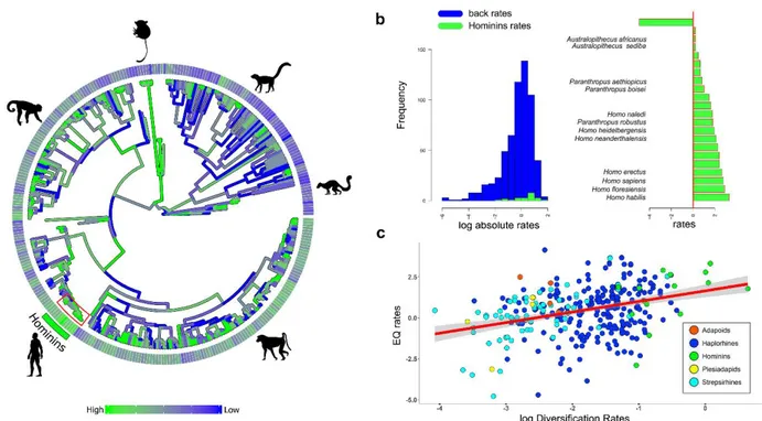
Figure 2. (a) Primate phylogeny. Colour gradient associated to the branches represent estimated rates of EQ evolution. The bars around the tree represent estimated diversification rates (DR). (b) Absolute rates of individual branches of the Hominins clade are collated in increasing rate value (green bars) and contrasted to the average rate computed over the rest of the tree branches (the vertical red line). Bars without names correspond to internal nodes. (c) Regression between encephalization quotient rates and diversification rates.
The image was generated by using the R package ggplot (http://ggplot2.org/) and our own R codes. Animal silhouettes were available under Public Domain license at phylopic (http://phylopic.org/), unless otherwise indicated. Specifically, Homo sapiens (http://phylopic.org/image/c089caae-43ef-4e4ebf26-973dd4cb65c5/),
Cebus (http://phylopic.org/image/156b515d-f25c-4497-b15b-5afb832cc70c/) available for reuse under the
Creative Commons Attribution 3.0 Unported (https://creativecommons.org/licenses/by/3.0/) image by Sarah Werning; Tarsius (http://phylopic.org/image/f598fb39-facf-43ea-a576-1861304b2fe4/); lemuriformes (http://phylopic.org/image/eefe8b60-9a26-46ed-a144-67f4ac885267/), available for reuse under Attribution-ShareAlike 3.0 Unported (https://creativecommons.org/licenses/by-sa/3.0/) image by Smokeybjb; Plesiadapis (http://phylopic.org/image/b6ff5568-0712-4b15-a1fd-22b289af904d/), available for reuse under Attribution-ShareAlike 3.0 Unported (https://creativecommons.org/licenses/by-sa/3.0/) image by Nobu Tamura (modified by Michael Keesey).
33
EQ values and rates are positively correlated with DR (slopephenotype = 0.434, pphenotype < 0.001; sloperate = 0.646, prate < 0.001; Fig. 2; Table S5). Furthermore, DR and EQ values are significantly correlated (p = 0.027; Table S5) when the effect of phylogeny is added as covariate in the regression model (PGLS).Body mass
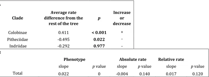
Results for body mass shows an increase in average rates in Colobine monkeys, whereas Pitheciids and Indriidae shows an opposite pattern. Furthermore, there is a general positive trend for body mass along Primate history (Table 4). For more details on trends in Colobinae, Pitheciids and Indriidae, and on SMA results see table S6 and S7. Eventually, we performed the same analysis focussing on hominins node (Table S8, S9).
A
Clade
Average rate difference from the
rest of the tree
p Increase or decrease Colobinae 0.411 < 0.001 + Pitheciidae -0.495 0.022 - Indriidae -0.292 0.977 - B
Phenotype Absolute rate Relative rate
slope p value slope p value slope p value
Total 0.022 0 -0.004 0.140 0.017 0.120
Table 4. Results for body mass. A) search.shift results; B) search.trend results for all Primates.
Pradel’s models
For both types (‘survival and seniority’ and ‘survival and growth rate’), the best model is the one where parameter estimates are function of EQ and sampling is allowed to change from one time bin to the next (Table 5). As models for seniority and growth rate are equivalent (DeltaAICc = 0.710), we retrieved estimates for speciation (1 - seniority), and extinction (1 - survival) rates from the former.
34
model npar AICc DeltaAICc weight Deviance
Phi(~EQ)p(~time*EQ)Lambda(~EQ) 130 1363.347 0.000 0.588 992.040 Phi(~EQ)p(~time*EQ)Gamma(~EQ) 130 1364.057 0.710 0.412 992.750 Phi(~time)p(~time)Lambda(~time) 187 1467.487 104.140 0.000 4.067 Phi(~1)p(~time)Lambda(~1) 65 1485.348 122.001 0.000 525.179 Phi(~1)p(~time)Gamma(~1) 65 1485.854 122.507 0.000 525.685 Phi(~EQ)p(~EQ)Lambda(~EQ) 6 1525.967 162.620 0.000 1513.772 Phi(~EQ)p(~EQ)Gamma(~EQ) 6 1533.310 169.963 0.000 1521.115 Phi(~time)p(~time)Gamma(~time) 187 1608.559 245.212 0.000 145.138 Phi(~1)p(~1)Gamma(~1) 3 1938.160 574.813 0.000 1125.062 Phi(~1)p(~1)Lambda(~1) 3 1938.160 574.813 0.000 1125.062
Table 5. Results for comparison of Pradel’s models applied on one million year time intervals. npar = number of parameters; AICc = corrected Akaike Information Criterion; DeltaAICc = the difference in the AIC value between each model and the model with the lowest AIC; weight = normalized Akaike weights; Deviance = models deviance.
In accordance with the best model, there is a linear relationship between extinction and speciation rate and EQ. We extracted regression coefficients from model results and computed extinction and speciation rates for each EQ values, hence for each species (Fig. 3 left). We therefore found a trend for increase in speciation rate and decrease in extinction rate with EQ. The intersection of the regression lines corresponds to EQ values in the range of early Primates species (Plesiadapids and Adapoids).
Eventually, we calculated the average rates value for each time interval (Fig. 3 right). We found an increase in speciation rate and a corresponding decrease in extinction rate starting from Early Oligocene. The distance between the curves accentuates at the beginning of Miocene.