Equilibrium in a two-agent Assignment Problem
Giovanni Felici
Istituto di Analisi dei Sistemi ed Informatica del CNR, Viale Manzoni, 30, Roma, Italy
E-mail: [email protected]
Website: www.iasi.rm.cnr.it/iasi/personnel/felici.html
Mariagrazia Mecoli
Università degli Studi di Roma ‘La Sapienza’, Roma, Italy
E-mail: [email protected]
Pitu B. Mirchandani
SIE, University of Arizona,
1127 E. James E. Rogers Way, Engineering Building 20, P.O. Box 210020 Tucson, AZ, USA
E-mail: [email protected]
Website: www.sie.arizona.edu/faculty/mirchandani.html
Andrea Pacifici*
Università degli Studi di Roma di Tor Vergata, Via del Politecnico, 1, Roma, Italy
E-mail: [email protected]
Website: www.disp.uniroma2.it/users/pacifici *Corresponding author
Abstract: In this paper we address a particular generalisation of the Assignment Problem (AP) in a Multi-Agent setting, where distributed agents share common resources. We consider the problem of determining Pareto-optimal solutions that satisfy a fairness criterion (equilibrium). We show that the solution obtained is equivalent to a Kalai–Smorodinsky solution of a suitably defined bargaining problem and characterise the computational complexity of finding such an equilibrium. Additionally, we propose an exact solution algorithm based on a branch-and-bound scheme that exploits bounds obtained by suitably rounding the solutions of the corresponding linear relaxation, and give the results of extensive computational experiments.
Keywords: competitive assignment; equilibrium; Pareto-optimality. Reference to this paper should be made as follows: Felici, G., Mecoli, M., Mirchandani, P.B. and Pacifici, A. (2009) ‘Equilibrium in a two-agent Assignment Problem’, Int. J. Operational Research, Vol. 6, No. 1, pp.4–26.
Biographical notes: Giovanni Felici is currently Tenured Researcher at the Isitituto di Analisi dei Sistemi ed Informatica of the Italian National Research Council, in Rome (Italy). His main area of expertise is operations research, subject in which he received his MSc at the University of Lancaster (UK) and his PhD at the University of Rome ‘La Sapienza’. His research interests cover integer optimisation, polyhedral methods, optimisation algorithms for data mining and their applications. He recently approached the promising field of research related with the mathematical models and algorithms for the solution of multi-agents optimisation problems in a competitive environment.
Mariagrazia Mecoli obtained her PhD Degree in Operations Research from the University of Rome ‘La Sapienza’ in 2005. Her primary research interests are in combinatorial optimisation with applications in logistics, transportation, and resource assignment. She is currently working at the Department of Statistics and Probability at the University of Rome, ‘La Sapienza’.
Pitu B. Mirchandani, Salt River Project Professor of Technology, Public Policy, and Markets, has joint appointments in the Department of Systems and Industrial Engineering and the Department of Electrical and Computer Engineering at the University of Arizona. He is the Director of the ATLAS Research Center. His expertise includes logistics, games and equilibria, design of decision/control systems, and their application in transportation and distribution. He received a Bachelor’s Degree and a Master’s Degree in Engineering from the University of California-Los Angeles, a Master’s Degree in Aeronautics and Astronautics, and a Doctorate in Operations Research from the Massachusetts Institute of Technology.
Andrea Pacifici is an Assistant Professor in operations research at the Engineering Faculty of the University of Rome Tor Vergata. He received a bachelor’s degree in Information Engineering and a PhD in operations research both at the University of Rome ‘La Sapienza’. His research is mainly concerned with algorithms design and computational complexity characterisation for combinatorial optimisation problems with applications to scheduling, logistics, manufacturing, telecom and multi-agent systems.
1 Introduction
The standard Assignment Problem (AP) consists in finding a minimum cost matching of jobs to machines. It is a well known combinatorial optimisation problem solvable in polynomial time (Bertsekas, 1981; Burkard, 2002; Khun, 1955). A considerable amount of literature, inspired by many practical applications and operations research models, addresses various extensions of AP. Among the others, we mention the Generalised Assignment Problem, where machines have capacities and each job has a size (see for instance Benders and van Nunen, 1983; Fisher et al., 1986; Higgins, 2001; Ross and Soland, 1975; Savelsbergh, 1997, and in particular, Cattryse and Wassenhove, 1992, for a survey of algorithms), and the class of Constrained Assignment Problems in which one has to find an optimal assignment while satisfying various kinds of side constraints (Aggarwal, 1985; Aboudi and
Nemhauser, 1991; Gupta and Sharma, 1981; Mazzola and Neebe, 1986; Punnen and Aneja, 1995). From the computational complexity standpoint, unlike the standard problem, most of these extensions fall in the class of N P-hard problems.
In this paper, we focus on a particular generalisation of AP in a Multi-Agent setting, where two agents have their own sets of jobs and want to assign them to a set of machines. Each agent wishes to minimise an objective function depending on the assignment costs of its own jobs only, thus competing for the usage of the shared machines. We refer to this class of problems as Competitive Assignment Problem (CAP).
Multi-agent systems have recently received an increasing amount of attention in the optimisation literature (Arbib and Rossi, 2000; Agnetis et al., 2004; Felici et al., 2004; Oliveira et al., 1999). These systems are comprised by distributed autonomous agents which share common resources. Since there is no central coordinator, the agents, in pursuing their objectives, may give raise to conflicts. If this is the case, in order to reach a compromise, the agents want to negotiate over a suitable subset of the feasible agreements (assignments) where a better assignment for one agent necessarily results in a worse assignment for the other. These kind of solutions are known as non-dominated or Pareto-optimal solutions. Throughout the paper we make use of the term Pareto-optimal or, briefly, PO solution.
Our problem also presents analogies with a special cooperative game with nontransferable utility, namely the two-person bargaining problem, originally introduced by Nash (1950). The classical axiomatic characterisations of bargaining solutions are based on the assumption that the set of feasible agreements is convex. In the literature, some studies address nonconvex bargaining problems, and present extensions of classical equilibrium solutions such as those by Nash and Kalai and Smorodinsky (1975). In this context, a number of alternative axiomatic characterisations and different solutions are given for the class of compact and comprehensive (nonconvex) set of agreements (Conley and Wilkie, 1991, 1996; Herrero, 1989; Lin, 1997) or for bargaining problems where the number of agreements is finite (Kaneko, 1980; Mariotti, 1998). However, our study is related to a particular class of finite, non-convex bargaining problem where the set of agreements is discrete. CAP may indeed be regarded as a two person bargaining problem where the set of the feasible agreements is discrete (and therefore nonconvex). In this paper, rather than providing an axiomatic characterisation of a bargaining solution, we aim at developing numerical methods to obtain a solution with desirable properties. We therefore • consider a generalisation of the Kalai–Smorodinsky solution, called Equilibrium
Assignment
• formulate the problem of finding such a solution as an integer program, namely the Equilibrium Assignment Problem (EAP)
• characterise its computational complexity • design and test an exact solution algorithm.
The paper is organised as follows. Section 2 introduces CAP and gives the main notation used throughout this paper. In Section 3, the definition of Pareto-optimal solution is given. Special PO solutions, called efficient solutions, are also introduced. Issues related to the problem of finding one or all the PO solutions are also discussed.
The definition of EAP, which is modelled as a {0, 1} integer program, is illustrated in Section 4. We show that this problem is N P-hard, and prove that an optimal solution of the linear relaxation of EAP is a Kalai–Smorodinsky solution. The latter solution is used to obtain primal (i.e., feasible solution values) and dual (i.e., lower) bounds that one may exploit in an exact algorithm to solve EAP. Such an algorithm, based on a branch-and-bound scheme, is illustrated together with rounding techniques devised to obtain the primal (upper) bound for EAP. Sections 5 and 6 present computational experiences: design of the experiments, solver tools and alternative strategies are discussed. Finally, conclusions are drawn and directions for future research are given in Section 7.
2 Problem statement
The standard AP consists in finding a minimum cost matching of n jobs with n machines, and can be formulated as follows:
min n ! i=1 n ! j=1 cijxij x∈ A (1) x∈ {0, 1}n×n
where cij∈ Z+is the cost of assigning job i to machine j; A is the assignment polytope,
A ="x∈ Rn×n: #n
i=1xij = 1, #nj=1xij = 1, x ≥ 0n×n$; the binary variable xij is
equal to 1 if job i is assigned to machine j and 0 otherwise.
Several methods for solving AP in polynomial time are known: some use linear programming techniques, exploiting the integrality of the assignment polytope (see Khun, 1955), while others use different combinatorial algorithms (see Bertsekas, 1981; Burkard and Cela, 1999; Gabow and Tarjan, 1989).
In this paper we consider two competing agents, referred to as Agent A and B, owning two disjoint sets of jobs to be assigned to a set M of n machines. Agent A is identified by the set of its jobs IA= {a1, a2, . . ., anA}, while Agent B by the set
of its jobs IB = {b1, b2, . . ., bnB}, with IA∩ IB= ∅, and (with no loss of generality)
nA+ nB= n.
The set of feasible solutions for CAP coincides with the set of feasible solutions for AP, i.e., formally, with the set of verticesExt(A) of the assignment polytope A.
We write an assignment x as x = (xA, xB) if we are distinguishing the vectors’
components corresponding to the jobs belonging to the two agents. Given a feasible assignment x, we denote by cA(x), cB(x) the assignment costs for Agent A and B,
respectively.
Let us call PAthe AP of Agent A, that is the problem of assigning its n
Ajobs to
the n machines minimising cA(x), and PB the corresponding problem for Agent B.
Both problems PAand PBare polynomially solvable as they are standard APs.
Let M∗
A, and MB∗, be the set of machines used in the optimal solution of problem
PA, and PB, respectively. If M∗
A∩ MB∗ = ∅, then there is no conflict in the usage of
the machines, and there is a unique trivial PO solution. On the contrary, the example below illustrates a case where conflicts arise on three machines.
Example 1: Consider the following instance of CAP, where nA= nB = 5,
M ={1, 2, . . . , 10}, and the costs for the two agents are given by the following two matrices: " cAij $= 2 3 4 5 4 3 2 4 7 7 3 5 3 4 6 4 2 5 6 6 3 4 3 3 5 8 5 5 5 8 5 6 3 2 6 6 6 1 4 7 3 4 4 5 6 6 6 7 8 6 " cBij $= 3 3 3 4 3 5 2 5 6 6 5 5 8 2 2 5 2 2 5 8 4 6 3 7 4 4 2 4 7 7 6 4 8 2 3 3 4 3 5 4 3 3 5 4 6 4 7 5 5 6 .
The optimal solution of PA is {(a
1, 6), (a2, 7), (a3, 4), (a4, 8), (a5, 1)}, where (ai, j)
indicates the matched pair, i = 1, . . . , nA, j ∈ M, and its value is 12. Analogously,
the optimal assignment of Agent B (solution of PB) is {(b
1, 2), (b2, 5), (b3, 7),
(b4, 4), (b5, 1)} with optimal value equal to 12. Then, MA∗ = {1, 4, 6, 7, 8}, and
M∗
B = {1, 2, 4, 5, 7}. Hence, in this case, there is a conflict on machines 1, 4, and 7.
3 Pareto optimality
When the intersection between M∗
Aand MB∗ is not empty, as in the Example 1, then it
makes sense to look for Pareto-optimal solutions, which are defined as follows. A feasible assignment x is Pareto-optimal if there is no other feasible assignment x#, with x#%= x, such that:
cA(x#) < cA(x), cB(x#) ≤ cB(x) or cB(x#) < cB(x), cA(x#) ≤ cA(x).
On the other hand, if such an assignment x# exists, then we say that x is dominated
and that x#dominates x.
We represent geometrically Pareto-optimal solutions in the cost space: given a feasible assignment x ∈ A we draw the point (cA(x), cB(x)) in the 2-dimensional
euclidean space. Hereafter, unless the context is not clear, we indicate both a PO assignment x and its image in the cost space with the term ‘Pareto Optimal solution’. We refer to the set {(cA(x), cB(x)) : x is a PO solution} as the Pareto-optimal frontier.
3.1 Extreme PO solutions
Unless we are in the trivial case, at least two PO solutions may be obtained with an easy procedure. First, observe that, for any PO solution x, cA(x) ≥ c∗A and cB(x) ≥ c∗B,
where c∗
Aand c∗Bare the optimal solution values of PAand PB. Suppose now that the
optimal solution x∗
Aof PAis unique and solve the problem of assigning the jobs of IB
to the machines in M\M∗
A. Call cB|Aits optimal value. Then the point(c∗A, cB|A) is a
PO solution; in fact, since PAhas a unique optimum, any possible improvement for
Agent B results in an increased cost for Agent A.
In general, the optimal assignment for one agent may not be unique. When two or more equivalent optimal solutions are available for one agent, we will assume that this agent always picks the solution leaving the best possible set of machines for the other agent. This makes the solution obtained Pareto-optimal. Suppose we want an optimal assignment for Agent A (so that it obtains a cost c∗
A) simultaneously
we are looking for an optimal solution ˜x of the following program: min{cB(x) :
cA(x) = c∗A, x∈ A ∩ {0, 1}n×n}. Indeed, we may find ˜x by solving another standard
AP where the objective is a suitable linear combination of the agents’ cost functions: KcA(x) + cB(x). Factor K should be large enough so that no decrease in costs from
the assignment of Agent B could drive the optimal solution toward a value that is no longer optimal for A. (Given that the cost coefficients are integer, we may choose, e.g., K > UBB
− LBBwhere UBBand LBBare upper and lower bounds for c B(x).)
In conclusion, the pair (c∗
A, cB|A) equals (cA(˜x), cB(˜x)), and the corresponding
solution ˜x = (x∗
A, xB|A) is Pareto-optimal. Symmetrically, the pair (cA|B, c∗B),
corresponding to solution (xA|B, x∗B), is Pareto-optimal. Therefore the following
observation holds.
Observation 2: Any PO solution x of an instance with costs cA(x) and cB(x) for Agent
A and B respectively, is such that c∗
A≤ cA(x) ≤ cA|Band c∗B≤ cB(x) ≤ cB|A.
Note that, in the special case when M∗
A∩ MB∗ = ∅ the problem admits a unique
Pareto-optimal solution x∗ and the two points (c∗
A, cB|A) and (cA|B, c∗B) coincide.
If this is not the case, the two PO points(c∗
A, cB|A), and (cA|B, c∗B) are the two extreme
points of the Pareto frontier.
Example 3: Referring to the instance of CAP given in Example 1, we have x∗A= {(a1, 6), (a2, 7), (a3, 4), (a4, 8), (a5, 1)}, and x∗B= {(b1, 2), (b2, 5), (b3, 7), (b4, 4),
(b5, 1)} and the optimal values c∗Aand c∗Bare both equal to 12.
By eliminating the set of machines optimally assigned to Agent B, MB, from
the set of machines available to Agent A, the conditioned assignment of Agent A, PA|B, becomes the problem of assigning the I
A jobs to the set of machines
M\MB= {3, 6, 8, 9, 10}. The solution to this standard AP is xA|B= {(a1, 6), (a2, 3),
(a3, 9), (a4, 8), (a5, 10)}, with value cA|B= 18. For Agent B, by solving PB|A we
obtain a conditioned value cB|A= 17 and the solution is xB|A= {(b1, 2), (b2, 5), (b3, 3),
(b4, 10), (b5, 9)}. In this case we have c∗A%= cA|Band c∗B %= cB|Aand the corresponding
two extreme points of the Pareto frontier are represented by (12, 17) and (18, 12). The other points composing the PO set are given by (13, 16), (15, 15), (16, 14), (17, 13); Figure 1 shows the values of the solutions in the PO set.
3.2 Number of PO solutions
Here we show that the number of Pareto-optimal assignments may grow exponentially with the size of the instance and therefore that, in general, it is not possible to generate all the PO points efficiently.
Proposition 4: The number of Pareto-optimal solutions of a CAP is not polynomially bounded.
Proof: To prove the proposition we build an instance where the number of PO solutions is exponential in the number of jobs. Assume that nA= nB= n2 (n even)
and that, for1 ≤ i ≤ n
2, 1≤ j ≤ n, cAij= cBij= cj = 2j−1, that is, the cost of assigning
It is straightforward to see that, given two different feasible assignment x and x#%= x
in A ∩ {0, 1}n×n, the following properties hold:
cA(x) + cB(x) = n ! j=1 cj= 2n− 1; (2) cA(x) %= cA(x#). (3)
For a given assignment x, let MA(x) denote the set of machines which the jobs of
Agent A are assigned to. From the above properties, for any two assignments x and x# such that M
A(x) %= MA(x#), cA(x) %= cA(x#). Moreover, if cA(x) > cA(x#) then
cB(x) < cB(x#) and, conversely, if cA(x) < cA(x#) then cB(x) > cB(x#). Hence, any
possible assignment for this instance is Pareto-optimal and there are as many PO pairs as the number of different possible subsets MA(x), i.e.,+nn
2
,= Ω+2n
n
,PO solutions. ! Figure 1 The PO frontier of Example 3 (see online version for colours)
3.3 Efficient PO points
For the developments to follow, we define a special subset of PO points in the cost space, those lying on the convex hull of the Pareto frontier, that we call efficient points. For instance, the extreme points of the Pareto frontier, given by the two points(c∗
A, cB|A) and (cA|B, c∗B) are efficient. In Figure 1, the two extreme PO points
(12, 17) and (18, 12) and the PO points (13, 16), (17, 13) are efficient, whereas (15, 15) and (16, 14) are not.
Differently from other PO solutions, any efficient point can be found by solving the following linear program for a given value of λ, 0 ≤ λ ≤ 1:
z(λ) = min λ! i∈IA ! j∈M cA ijxij+ (1 − λ) ! i∈IB ! j∈M cB ijxij x∈ A (4) x∈ {0, 1}n×n.
Due to this property it is possible to verify in polynomial time if a feasible assignment is efficient (see Felici et al., 2004). However, it is important to observe that the number of efficient points is not polynomially bounded (in fact, in the proof of Proposition 4, all the PO points are efficient.)
3.4 Finding a PO solution
A possible approach (see Agnetis et al., 2004) to determine a PO assignment for CAP relies on the solution of a suitable integer program.
Given the sets IA, IB, the two objective functions cA(·), cB(·), and an integer Q
such that c∗
B≤ Q ≤ cB|A, we consider the problem of finding an assignment x∗such
that Agent A gets the best assignment given that Agent B will accept an assignment of cost up to Q. We refer to this problem as Constrained Problem (CP). CP can be formulated as an integer linear program:
zA(Q) = min cA(x)
x∈ A (5)
cB(x) ≤ Q
x∈ {0, 1}n×n.
It is easy to show that it is always possible to obtain a PO solution(¯cA, ¯cB) with
¯cA≤ zA(Q)
¯cB ≤ Q
by means of a binary search on the Q values in the interval [c∗ B, Q].
Observation 5: If -A is a solution algorithm for CP that runs in O(f (n)) time, then it is possible to use -A in a binary search framework to obtain a PO solution in O(f (n)· log(cB|A− c∗
B)) time.
The following Proposition 6 shows that CP is a N P-hard problem. Hence using CP to determine all the PO solutions, even when they are polynomially many, turns out to be a non-polynomial procedure.
Proposition 6: CP is N P-Hard.
Proof: We prove that CP, as formulated in equation (5), is binary N P-hard by making use of a reduction from the well known PARTITIONproblem: given n nonnegative
integers w1, w2, . . . , wnwith#ni=1wi= W , find, if it exists, a subset S ⊆ {1, . . . , n}
such that#i∈Swi= 12W . PARTITION remains N P-hard if we restrict S to have
cardinality equal ton
2 (see, e.g., Garey and Johnson, 1979).
We consider the following instance of CP where the cost cij of assigning a job i
to a machine j is given by wjfor every i ∈ IA∪ IB, and j ∈ M. The number of jobs
owned by Agent A is nA= n2; M = {1, . . . , n}. Clearly c∗A= c∗B since they are both
equal to the sum of then
2 lowest wj’s; while cA|B= cB|Ais equal to the sum of the n2
The decision form of CP is the following: given two nonnegative real numbers ¯c and Q, find if there is a solution x ∈ A ∩ {0, 1}n×n, such that c
A(x) ≤ ¯c and
cB(x) ≤ Q. Note that cA(x) + cB(x) = W . If we choose ¯c = Q = W/2, the decision
problem is equivalent to the problem of determining a subset S ⊆ M such that |S| = n 2
and#j∈Swj= W2. This is equivalent to the restricted PARTITIONproblem defined
above. !
4 Equilibrium between agents
In this section we focus on the problem of determining a special PO solution that provides an equilibrium of the system.
We are showing that this problem can be seen as a special bargaining problem with two players and that the optimal solution of a suitably defined linear program turns out to be a Kalai-Smorodinski solution of such a bargaining problem which provides bounds to the equilibrium we are looking for. Below we provide a formal description and a formulation for the problem of finding such an equilibrium. Also, we analyse whether an equilibrium always exists and/or it is unique.
Recall that the best and the worst possible PO alternative for one agent, say Agent A, are c∗
Aand cA|B(respectively, c∗Band cB|A, for Agent B). Given an assignment
x, we define the ratio of Agent A, rA(x) (of Agent B, rB(x)) as:
rA(x) =cA(x) − c ∗ A cA|B− c∗A . rB(x) = cB(x) − c ∗ B cB|A− c∗B / . (6)
These ratios are normalised distances of the agents’ costs from their respective optimal values. Our definition of equilibrium solution exploits these ratios: the more similar the ratio values of a PO solution x are, the better is the compromise. In particular, if a PO solution x exists with rA(x) = rB(x), then x represents a best compromise. In the cost
space, the ideal points where rA(x) = rB(x) define a line that we call equilibrium ray.
In conclusion, we define the Equilibrium Assignment Problem (EAP) as follows. r∗= min{max{rA(x), rB(x)} : x ∈ A, x ∈ {0, 1}n×n}. (7)
To solve EAP, we may equivalently address two different integer linear problems. With reference to the cost space representation, the idea is to determine the two closest PO solutions to the equilibrium ray. This is modelled by the following integer program for the minimisation of rA:
rA∗ = min rA(x)
x∈ A (8)
rA(x) ≥ rB(x)
x∈ {0, 1}n×n.
Symmetrically, we obtain the second linear program for minimising rB. Clearly,
r∗= min{r∗ A, rB∗}.
4.1 Computational complexity issues
In what follows we will study Problem 8. We show below that EAP is N P-Hard. Proposition 7: The Equilibrium Assignment Problem is N P-Hard.
Proof: We follow the same approach as in the proof of Proposition 6. For the same instance used in that proposition, the decision form of EAP, as defined in equation (8), is the following: given¯c ∈ R+, find if there is a solution x ∈ A ∩ {0, 1}n×n, such that
cA(x) ≥ cB(x) and cA(x) ≤ ¯c. By definition, cA(x) = W − cB(x), thus cA(x) ≥ cB(x)
can be rewritten as cA(x) ≥ W2. Let us choose¯c = W/2; the decision problem is thus
equivalent to the problem of determining a subset S ⊆ M such that#j∈Swj =W2
and this is equivalent to the restricted PARTITIONproblem defined in the proof of
Proposition 6. !
The complexity of the problem implies that a polynomial exact solution algorithm is unlikely to exist.
In the following sections we first analyse a linear relaxation of EAP and develop a solution method based on branch-and-bound where a lower bound obtained starting from the solution of the linear relaxation is exploited.
4.2 Linear relaxation of EAP
Consider now the following problem (LEAP), which is a linear relaxation of EAP. rLP = min rA(x)
x∈ A (9)
rA(x) ≥ rB(x)
0 ≤ xij ≤ 1 i ∈ IA∪ IB, j∈ M.
In general, the solution value rLP of LEAP is a lower bound for EAP. We denote
by A# the non-empty polytope defined by its feasible solutions: A#= A ∩ R≥,
where R≥= {x ∈ Rn×n: r
A(x) ≥ rB(x)}. For the developments to follow, let also
R== {x ∈ Rn×n: r
A(x) = rB(x)}.
In the following we characterise the properties of the optimal solutions of Problem 9.
Proposition 8: Let x∗be an optimal solution of Problem 9. Then r
A(x∗) = rB(x∗).
Proof: We first rule out the trivial case when cA(x∗) = c∗A. Clearly, we have rA(x∗) =
rB(x∗) = 0 and x∗is the unique PO solution.
Let x∗be an optimal solution of Problem (9) for which c
A(x∗) > c∗A(i.e., we have
more than one PO solution), and suppose, by contradiction, that the proposition does not hold, that is rA(x∗) > rB(x∗).
Since Problem (9) is a linear program, then x∗∈ Ext(A ∩ R≥), that is, x∗ is a
vertex of the the polytope that defines the feasible region of Problem (9). Given that x∗∈ Ext(A ∩ R=) contradicts r
A(x∗) > rB(x∗), it must be x∗∈ Ext(A). Hence x∗is
Let˜x be an assignment corresponding to (c∗
A, cB|A) in the (cA, cB) plane. We have
rA(˜x) ≤ rA(x∗) and ¯x %= x∗. Consider a convex combination of x∗and˜x, x = λx∗+
(1 − λ)˜x, with 0 ≤ λ ≤ 1. Clearly x ∈ A and, for small enough values of λ, rA(x) ≥
rB(x). In conclusion, as c∗A< cA(x) < cA(x∗), x is a feasible solution of Problem (9)
with rA(x) < rA(x∗), thus, x∗is not optimal and this is a contradiction. !
By very similar arguments one can show that no feasible assignment may improve the cost for Agent B without increasing cost for Agent A and thus the following proposition holds.
Proposition 9: Let x∗ be an optimal solution of LEAP (9). Then no feasible
assignment x exists such that cA(x) ≤ cA(x∗) and cB(x) < cB(x∗), or cA(x) < cA(x∗)
and cB(x) ≤ cB(x∗). In the special case when x∗is integer then it is Pareto-optimal.
We will now characterise the setExt(A#) of the vertices of the polytope defined by the
feasible solutions of LEAP.
We first recall some general concepts of polyhedral theory as illustrated in Nemhauser and Wolsey (1988). A polyhedron is the intersection of a finite set of half spaces; let P = {x ∈ Rn; Ax ≤ b} be a polyhedron, where (A, b) is an m × (n + 1)
matrix. Let(A=, b=) be the submatrix corresponding to the rows i ∈ {1, . . . , m},
such that aix = b
ifor all x ∈ P . Given ¯x ∈ P , let A=x¯ be the submatrix corresponding
to the rows i ∈ {1, . . . , m}, such that ai¯x = b i.
The dimension of P is dim(P ) = n − rank(A=). Below we will assume that the
polyhedron P is full-dimensional, that is dim(P ) = n. Given P %= ∅, and an inequality πx≤ π◦satisfied for all x ∈ P , then the polyhedron F = {x ∈ P : πx = π◦} is called
face of P . An extreme point x of P is a 0-dimensional face of P , which means that, given thatdim(P ) = n, rank(A=
x) = n, and there are n linear independent constraints
that are tight at x. An edge of a polyhedron P is a 1-dimensional face of P , and it is given by the set of points x for which rank(A=x) = n − 1.
Proposition 10: Consider the full-dimensional polyhedron P = {x ∈ Rn; Ax ≤ b},
the half-space H = {x ∈ Rn, dx
≤ c} and the polyhedron P# = P ∩ H, with P#%= ∅.
Then, either P#is a face of P or dim(P ) = dim(P#).
Proof: It follows trivially from dim(P ) = n − rank(A=), and P# %= ∅. !
Proposition 11: Consider the full-dimensional polyhedron P = {x ∈ Rn; Ax ≤ b},
the half-space H = {x ∈ Rn, dx≤ c} and the polyhedron P# = P ∩ H, with P#%= ∅.
Then, any extreme point x∗∈ P#lies on an edge of P .
Proof: First we consider the case in which P#is a face of P . In such case x∗is a vertex
of P and the Proposition follows.
If P#is not a face of P , consider two sub-cases:
a P#= P ∩ H = P ; then the statement of the proposition is trivially satisfied since
b P#= P ∩ H ⊂ P ; then from Proposition 10 dim(P ) = dim(P#) = n, since P#is
not a face of P . One of the two following possibilities must hold:
i dx∗< c. Given that x∗is extreme point of P#, and thatdim(P#) = n, then
x∗satisfies at equality the n constraints. Therefore it must be Ax∗= b.
It follows that x∗is an extreme point of P .
ii dx∗= c. As above, x∗satisfies at equality exactly(n − 1) constraints
belonging to P . This trivially implies that x∗lies on an edge of P . !
From the above polyhedral considerations, the following results hold.
Proposition 12: Given A, the assignment polytope, and A#, the polytope described
by the feasible solutions of LEAP, for any vertex x∗of A#we have:
i x∗can be written as x∗= fx#+ (1 − f)x##, 0≤ f ≤ 1, where x#and x##are two
adjacent vertices of A, with x#∈ A#and x##∈ A/
ii Let x∗= {x∗
ij}i=1,... ,n
j=1,... ,n. Then x ∗
ijhas at most two non-zeroes for each row i and
column j.
Proof: (i) Proposition 11 holds, thus x∗lies on an edge of A. By definition, every
point on an edge can be written as linear combination of its extremes. Thus, given x#, x##, x#%= x##, extreme points of A, we have x∗= fx#+ (1 − f)x##, f > 0. Since x∗is
an extreme point of A#, then both x#, x##cannot be elements of A#.
(ii) This result follows from the matrix structure of feasible assignments x#and x##,
since any linear combination of two assignment solutions cannot have more than two
positive elements for each row and column. !
4.3 LEAP and Kalai–Smorodinsky solutions
In this subsection we briefly provide an interpretation of the optimal solution of LEAP in the context of classical game theory.
We refer to the definition of (convex) bargaining problem given by Nash (1950). Here, two agents aim to maximise their utilities in bargaining, measured as numerical payoffs. The problem consists of a pair(F, d) where F is a nonempty, compact, and convex set of feasible agreements, and d ∈ F is the disagreement point, i.e., the worst possible payoff pair. A bargaining solution φ(F, d) is a rule that assigns a feasible agreement to each bargaining problem. Nash defined a list of five axioms that a bargaining solution ought to satisfy ((i) Strong efficiency, (ii) Individual rationality, (iii) Scale covariance, (iv) Symmetry, and (v) Independence of irrelevant alternatives), and he showed that there exists a unique solution satisfying the five axioms. This solution is usually referred to as Nash bargaining solution of problem (F, d) (see Nash, 1950 for the details).
Starting from that seminal work, various axiomatic characterisation of a bargaining solution have been proposed in the game theory literature. In particular, due to many criticisms about the suitability of the Axiom (v), Kalai and Smorodinsky, later in 1975, replaced it with the (vi) Individual monotonicity axiom
(see Kalai and Smorodinsky, 1975). Kalai and Smorodinsky proved that there is a unique solution satisfying axioms(i), . . . , (iv), (vi), and this is
arg max0x1: x1− d1
u1− d1 =
x2− d2
u2− d2; x ∈ F
1
i.e., a particular PO solution lying on the segment whose extrema are the disagreement point d and the ideal point u. According to many authors, a Kalai–Smorodinsky solution “seems to be a more solid candidate for a general principle for the choice of outcome” (Hougaard and Tvede, 2003).
We now introduce a two-person bargaining problem(FLEAP, dLEAP) associated
to a given instance of LEAP, where the payoff function is given in terms of the cost functions of LEAP. For any (possibly fractional) assignment x, solution of LEAP, the payoff of Agent A is fA(x) = cA|B− cA(x) and, similarly, that of Agent B
is fB(x) = cB|A− cB(x). Each agent wishes to maximise her own payoff. Now,
the set of feasible payoffs for the agents is given by the set of points FLEAP=
{(fA(x), fB(x)) : x ∈ A}. Let the disagreement point be dLEAP = (0, 0), and consider
the ideal point uLEAP given by uLEAP = (cA|B− c∗A, cB|A− c∗B). Such situation can
be also interpreted as the problem where two players, A and B, bargain over the set of feasible assignments A in order to minimise each cost function, i.e. cA(x) or cB(x).
In this case the disagreement point corresponds to the worst assignment they both can get, given the presence of the other player, that is d = (cA|B, cB|A), and the ideal
point corresponds to the assignment such that cA(x) = c∗A, cB(x) = c∗B.
The Kalai–Smorodinsky solution for such a bargaining problem is given by
xKS = arg max 0 fA(x) : fA(x) cA|B− c∗ A = fB(x) cB|A− c∗ B ; x ∈ A1
Consider now LEAP and its optimal solution x∗. Due to Proposition 8, it follows
that x∗= arg min{r
A(x) : rA(x) = rB(x) : x ∈ A}. Then, by definition of fAand fB
it turns out that:
x∗= arg min{rA(x) : rA(x) = rB(x); x ∈ A}
= arg max{1 − rA(x) : 1 − rA(x) = 1 − rB(x); x ∈ A} = xKS.
In conclusion the following property holds.
Observation 13: The optimal solution x∗ of LEAP corresponds to
a Kalai–Smorodinsky solution φ(F, d), where F = {(cA|B− cA(x), cB|A− cB(x)) :
x∈ A} and d = (0, 0).
4.4 Bounds for the equilibrium problem
In this section we discuss procedures to obtain a good upper bound for EAP. Such bound is determined by simply rounding an optimal fractional solution x∗ of
LEAP which produces two different integer solutions (i.e., feasible assignments) x#
and x##. We next describe such procedure and show some properties of the upper
solutions obtained with the rounding procedure: to this purpose we make use of the graph and the matrix representations of feasible assignments. We then show some properties of the associated costs and relate them to the set of PO solutions.
Finally, in Section 4.4.3 we give the expression of the lower bound used in our enumeration scheme.
4.4.1 Rounding procedure
Any solution of an AP, i.e., an extreme point of A, can be represented by a subset of pairwise disjoint arcs in a complete bipartite graph, which we refer to as G, with all the arcs ij, i ∈ IA∪ IB, j ∈ M, with cost cij. (We use the terms arcs and nodes
with reference to an undirected graph, to distinguish them from vertices and edges of polyhedra.)
Similarly, recalling Proposition 12, an optimal solution of LEAP and, in general, any point lying on an edge of the polytope A, may be represented as a 2-matching, that is, a subgraph of G where each node has degree at most two. We will prove that, in our case, such a 2-matching is the union of a standard matching and a single, possibly empty, cycle.
Call G(x∗) the subgraph of G representing an optimal solution x∗of LEAP. G(x∗)
contains all the nodes of G (i.e., IA∪ IB∪ M) and the arcs ij such that x∗ij > 0.
The number of arcs of G(x∗) incident to node i ∈ I
A∪ IB(j ∈ M) equals the number
of fractional components of row i (or column j) in the matrix representation of x∗.
As stated in Proposition 12, if a row i (or column j) has non integer components, then there are exactly two of such components whose values are equal to, say, f and 1 − f, with0 < f < 1. As a consequence, every node i ∈ IA∪ IB (or j ∈ M) in G(x∗) has
degree at most two.
Let us denote each arc in G(x∗) corresponding to a variable having value 0 < f ≤ 1
as a f-arc.
Consider the subgraph of G(x∗) induced by all the nodes having degree two. It is not
hard to see that this subgraph must be a collection of even cycles with alternating f and (1 − f)- arcs. In conclusion, G(x∗) is given by a collection of pairwise disjoint arcs with
value 1 (1-arcs) and alternating cycles with f-arcs and (1 − f)-arcs (corresponding to the fractional variables).
In the following proposition we will prove a property of G(x∗) useful for
constructing the rounded solutions.
Proposition 14: The graph G(x∗) representing an optimal solution x∗ of LEAP
contains at most one cycle.
Proof: In the trivial case when x∗is integer, the set of edges of G(x∗), denoted as
E(G(x∗)), is a matching and there are no cycles.
Suppose x∗ has non-integer components and, by contradiction, that G(x∗)
contains at least two cycles. Let C1⊂ E(G(x∗)) be one of such cycles, and
C2⊂ E(G(x∗)) be the set of the edges of all the other possible cycles (C2%= ∅).
The components of x∗corresponding to the edges of C1∪ C2are fractional while all
the other components are integer.
Given a cycle C ⊆ E(G(x∗)), since arcs in C have alternating values f and 1 − f,
let us call FCthe set of f-arcs of C and FCthe set of(1 − f)-arcs in C. Additionally,
Assume first the case when all the f values are the same in the different cycles. Then x∗is as follows: x∗ij = f if ij ∈ FC1∪ FC2, (1 − f) if ij ∈ FC1∪ FC2, 1 if ij ∈ H, 0 otherwise.
Consider now the four vertices x#, x##, xL, and xRof A, defined as follows:
x∗ij = 6 1 if ij ∈ H ∪ FC1∪ FC2, 0 otherwise. x ## ij= 6 1 if ij ∈ H ∪ FC1∪ FC2, 0 otherwise. xL ij = 6 1 if ij ∈ H ∪ FC1∪ FC2, 0 otherwise. x R ij= 6 1 if ij ∈ H ∪ FC1∪ FC2, 0 otherwise.
We have x∗= fx#+ (1 − f)x##and x#, x##are the two adjacent vertices of A that define
the edge where x∗lies. Consider now the point xM =1
2x#+12x##. Note that xM lies
on the same edge where x∗lies. But xM can also be expressed as xM = 1
2xL+12xR,
i.e., this point is a convex combination of both x#, x## and xL, xR. But xL and xR
are feasible assignments, and thus vertices of A. Consequently, xM and therefore x∗,
do not lie on an edge of A which contradicts Proposition 12. Hence C2must be empty.
Similar arguments hold for the case where the f values are different for distinct
cycles. !
On this grounds, the component ij of an optimal solution x∗of LEAP is equal to:
x∗ij = f if ij ∈ FC∗, (1 − f) if ij ∈ FC∗, 1 if ij ∈ H, 0 otherwise (10)
where C∗is the single, possibly empty, cycle defined by the fractional components in
x∗. When x∗is not integer, we may obtain two different feasible matchings, x#and x##, with the following rounding procedure,
x#ij = 6 1 if ij ∈ H ∪ FC∗, 0 otherwise. x ## ij= 6 1 if ij ∈ H ∪ FC∗, 0 otherwise. (11)
It is easy to see that one of these assignments is feasible for Problem 8 while the other is not (i.e., the constraint rA(x) ≥ rB(x) is violated).
4.4.2 Quality of the rounded solutions
To illustrate the characteristics of the solutions obtained using the rounding procedure we need to refer to their mapping into the(cA, cB) space. When x∗is not integer, then
x# %= x∗%= x##. In this case, we assume, with no loss of generality, that r
A(x#) < rB(x#),
and rA(x##) > rB(x##).
Observation 15: The mapping of an optimal solution x∗ of LEAP on the
(cA, cB)-plane lies on the segment whose extreme points are (cA(x#), cB(x#)) and
(cA(x##), cB(x##)).
Proposition 16: The rounded solutions x#and x##are Pareto-optimal.
Proof: We prove that x#is Pareto-optimal. The result holds, by symmetry, for x##.
Let us suppose, by contradiction, that x#, for which r
A(x#) < rB(x#), is dominated.
Then there exists at least one feasible assignmentˆx that dominates x#, and we have:
cA(ˆx) ≤ cA(x#), cB(ˆx) < cB(x#) or (12)
cB(ˆx) ≤ cB(x#), cA(ˆx) < cA(x#). (13)
Suppose, without loss of generality, that equation (12) holds. Given Propositions 8 and 9, we have c∗
B< cB(ˆx) < cB(x#) and rA(ˆx) < rB(ˆx). Consider now x##, for which
rA(x##) > rB(x##), and the solution ˜x = λˆx + (1 − λ)x##, with0 < λ < 1. Therefore,
cA(˜x) = λcA(ˆx) + (1 − λ)cA(x##) and cB(˜x) = λcB(ˆx) + (1 − λ)cB(x##). Hence, due
to equation (12), cB(˜x) < λcB(x#) + (1 − λ)cB(x##) = cB(x∗). From definition of
rB(x), this implies rB(˜x) < rB(x∗); and since, from Proposition 8, rA(˜x) = rB(˜x) and
rA(x∗) = rB(x∗), it follows that rA(˜x) < rA(x∗) which contradicts that x∗is optimal
for LEAP. !
Proposition 17: The two solutions provided by the rounding procedure are efficient points.
Proof: We have to prove that, in the (cA, cB)-space, no PO points lie below the line
passing through the projections of x# and x## (as defined above) in the cost space.
By contradiction, suppose that there is such a point y: then either rA(y) < rB(y) or
rA(y) > rB(y), since it cannot be rA(y) = rB(y), otherwise x∗would not be optimal
for LEAP. Suppose that rA(y) > rB(y), we may thus identify a point ˜x = λy + (1 −
λ)x# such that ˜x ∈ A and r
A(˜x) = rB(˜x), for some 0 < λ < 1. Then ˜x would also
satisfy rA(˜x) < rA(x∗), contradicting that x∗is an optimal solution of LEAP. The case
rA(y) < rB(y) is symmetrical. !
As a consequence of this result, given an optimal fractional solution x∗of LEAP, x##
is an upper bound to problem EAP and therefore the only possible optima of EAP are the assignments x such that cA(x∗) ≤ cA(x) ≤ cA(x##) and cB(x##) ≤ cB(x) ≤ cB(x∗),
and are above the segment connecting the projections of x∗and x##in the cost space.
4.4.3 Lower bound for the equilibrium problem
As mentioned in Section 1, research on constrained APs (Aggarwal, 1985; Brans et al., 1972; Kennington and Mohammadi, 1994; Mazzola and Neebe, 1986; Rosenwein, 1991) often makes use of Lagrangean relaxations to produce strong lower bounds.
The EAP is a standard AP with the single additional constraint rA(x) ≥ rB(x).
the Geoffrion’s integrality property (Geoffrion, 1974) since the feasible region is the assignment polytope. As a consequence, the best Lagrangean bound cannot be better than that obtained through linear relaxation. Therefore, in the branch-and-bound scheme to solve EAP, we make use of the lower bounds provided by the LP’s.
In the case of integer costs cA
ijand fractional solution x∗of LEAP, we may further
improve these bounds using the following lower bound: rA∗ ≥ ,c
A(x∗)- − c∗A
cA|B− c∗A
.
5 Computational experience
Our branch-and-bound scheme (in the following referred to as EAP_bb) has been implemented using the bounds described in Sections 4.4 and 4.4.3 in the default CPLEX 8.0 branching scheme via callback functions (see ILOG Inc., 2003). We compared the solution produced by our algorithm with those by the default CPLEX branch and cut on a series of randomly generated test instances, varying the number of jobs for each agent (nA, nB) and the intervals from which costs are
generated.
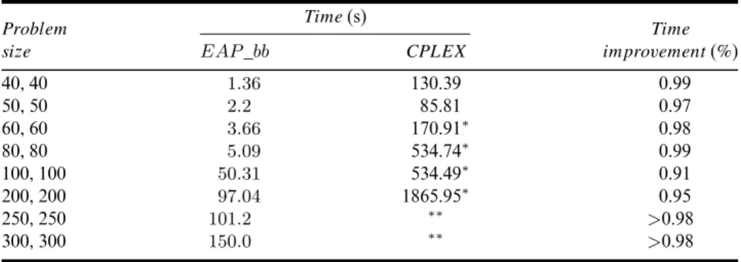
In a first set of experiments, whose results are reported in Table 1, we compared our algorithm and the default CPLEX branch and cut implementation, in terms of CPU times and effectiveness. Each one of the eight classes has the same size (which is reported in the first column). The results are average values over 30 instances for each class (three disjoint cost ranges were considered and, for each cost range, ten different randomly generated instances were solved). The average CPU times (in seconds) needed by EAP_bb and default CPLEX 8.0 are reported. Results marked with ‘∗’ indicate that the average values are only relative to those subsets of instances
where the optimal solution is obtained within a given time limit of 3600 s; whereas mark ‘∗∗’ indicates that the algorithm did not reach the optimum within the same time
limit, and the average times needed to find the best feasible solutions are presented. Table 1 Time comparisons between EAP_bb and CPLEX 8.0. The results are relative to averages
over different cost ranges and randomly generated instances Time (s)
Problem Time
size EAP _bb CPLEX improvement (%)
40, 40 1.36 130.39 0.99 50, 50 2.2 85.81 0.97 60, 60 3.66 170.91∗ 0.98 80, 80 5.09 534.74∗ 0.99 100, 100 50.31 534.49∗ 0.91 200, 200 97.04 1865.95∗ 0.95 250, 250 101.2 ∗∗ >0.98 300, 300 150.0 ∗∗ >0.98
EAP_bb improves the computational times upon CPLEX significantly: this is particularly evident for the largest instances of problems; our algorithm takes, on the average, less than 3 min to obtain an optimal solution while CPLEX takes hours.
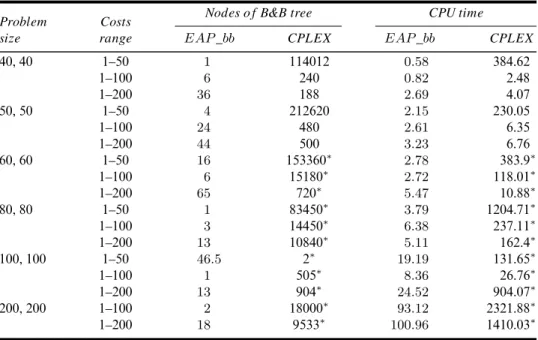
In Table 2, the number of nodes of the branch-and-bound tree (measuring memory occupation) and CPU times are reported. Moreover the results relative to different cost ranges are presented on separate rows. We may notice how using improved upper and lower bounds turns out in a dramatic decreasing of the number of nodes generated in the enumeration scheme. More surprisingly, in both algorithms, the number of nodes is highly sensitive to the cost ranges.
Again, also in Table 2, mark ‘∗’ indicates that we report average values only relative
to the instances where the optimal solution is obtained within a given time limit of 3600 s; whereas mark ‘∗∗’ indicates that the algorithm did not reach the optimum within
the same time limit and the average times needed to find the best feasible solutions are presented.
Table 2 Time and memory comparisons between EAP_bb and CPLEX 8.0. The results are relative to averages over randomly generated instances
Nodes of B&B tree CPU time Problem Costs
size range EAP _bb CPLEX EAP _bb CPLEX
40, 40 1–50 1 114012 0.58 384.62 1–100 6 240 0.82 2.48 1–200 36 188 2.69 4.07 50, 50 1–50 4 212620 2.15 230.05 1–100 24 480 2.61 6.35 1–200 44 500 3.23 6.76 60, 60 1–50 16 153360∗ 2.78 383.9∗ 1–100 6 15180∗ 2.72 118.01∗ 1–200 65 720∗ 5.47 10.88∗ 80, 80 1–50 1 83450∗ 3.79 1204.71∗ 1–100 3 14450∗ 6.38 237.11∗ 1–200 13 10840∗ 5.11 162.4∗ 100, 100 1–50 46.5 2∗ 19.19 131.65∗ 1–100 1 505∗ 8.36 26.76∗ 1–200 13 904∗ 24.52 904.07∗ 200, 200 1–100 2 18000∗ 93.12 2321.88∗ 1–200 18 9533∗ 100.96 1410.03∗
6 Testing the equilibrium strategy
In this section we analyse the quality of the equilibrium solution for CAP. Rather than addressing the efficiency of the algorithm used to find the equilibrium solution, we try to evaluate the suitability of the equilibrium approach in a 2-agents competition. In other words, one may question why an agent should find convenient to settle on an equilibrium solution. Here we try to set a specific experimental framework and draw some partial conclusions from the results.
We assume that two agents compete for the assignment of resources in a dynamic environment, where they are given more that one instance of the AP, and that the costs related with this assignment vary for each instance. We also refer to each instance of the problem as a game. Such situation may well represent realistic settings where the costs of consecutive games (biddings, market shares, task assignments) are affected
from external factors that are out of the agents’ control. In these settings the agents have to choose a strategy, that is, a rule to solve each instance of the assignment.
In our experiments we compared the following three simple strategies: • Equilibrium Strategy (ES), where the two agents agree over the equilibrium
solution, that is, an EAP is solved for each game.
• Global Optimal Strategy (OS), where the agents agree to choose the assignment with global minimum cost, eventually sharing the differential benefits at the end of each game.
• Alternate Strategy (AS), where the two agents solve the AP sequentially, the first one choosing the resources in an optimal way among all available resources, and, the second among those that are not used by the first one. In this case, the first decisor is selected by tossing a coin before each game.
We have set the following experiments. First, we generate a number of games where the assignment costs for the two agents are chosen at random according to the uniform distribution in a given interval. Second, we solve each game using the three strategies. Third, we compare the costs for the two agents (A and B) considering their average and variance over all the generated games.
We have considered different sizes of the APs, expressed as the number of resources to be assigned to the two agents, namely, 50, 100, 150, and 200 (in the following referred to as n); for each possible size the assignment costs have been generated randomly in the intervals(0, 4n) (‘small’) and (0, 8n) (‘large’). For each size and cost range, we have generated 300 APs, and solved them with the three strategies. The results are summarised in Table 3, where the first column reports the size of the AP (n) and the second column the interval used to generate the costs. The following three columns report the average cost for Agent A under the ES, OS and AS strategies. Columns six to eight report the same data for Agent B.
Obviously, as it might be expected, on the average the OS is the best in terms of final costs. It should be noticed that the average values of the costs for the two agents are also very close, under this strategy. The reason of this fact is related to the high number of instances (300) over which average are computed and to the uniform distribution used for the assignment costs cij. In a real setting, when the number of games between
two competitors is limited, this would be equivalent to require to transfer some of the utility at given time intervals, i.e., it assumes that the utility of the games is fully represented by the costs of the assignment. This is in fact a strong assumption in most cases.
The results highlight that, on the average, the distance between the Global Optimal and the Equilibrium strategies is actually small. An interpretation of this fact leads to conclude that the ES, in the long run, is not significantly worse than the OS in terms of global costs; but it is, by far, easier to implement in a competitive setting.
The AS, on the contrary, exhibits the largest costs for all problem sizes and cost types. Thus, in the long run and if agents have equal probability to win, it is convenient to settle on the equilibrium solution rather than simply compete to be first in the decision making process. Additionally, a strategy that exhibits low variance may be preferable to another that does not: as, in most cases, decision makers are interested in reducing uncertainty and having a steady behaviour in different games.
In Table 4, the information about the cost standard deviations, for the same set of experiments of Table 3, are reported. Not surprisingly, the ES performs with the lowest standard deviation, and results are more stable even when compared to the optimal one. It is important to stress that these comparisons are related with the average costs of A and B over a significantly large number of games (300). However, with reference to the results reported here, one may conclude that an ES, at least in the long run, stands as an interesting, perhaps easier to implement in a real world setting, alternative position with respect to total competition (AS) or total collaboration (the OS) scenarios. Table 3 Average costs for Agents A and B under Equilibrium Strategy (ES), Global Optimal
Strategy (OS), and Alternate Strategy (AS) Strategies
Agent A Agent B n Cost range ES OS AS ES OS AS 50 Small 175.33 170.40 218.23 172.50 171.92 230.99 50 Large 337.26 332.91 415.62 329.56 322.32 436.60 100 Small 350.31 349.27 464.11 346.90 342.94 447.75 100 Large 679.06 670.49 905.48 671.67 668.12 871.18 150 Small 527.35 525.67 718.88 527.16 523.54 663.40 150 Large 1010.38 1003.61 1391.70 1022.33 1018.34 1295.90 200 Small 705.54 705.57 941.70 708.80 703.73 925.32 200 Large 1363.24 1358.20 1819.37 1354.98 1349.13 1776.77
Table 4 Cost standard deviations for Agents A and B under Equilibrium Strategy (ES), Global Optimal Strategy (OS), and Alternate Strategy (AS) Strategies
Agent A Agent B n Cost range ES OS AS ES OS AS 50 Small 24.47 26.33 103.73 25.10 28.15 103.43 50 Large 49.44 52.76 199.84 45.86 52.23 198.49 100 Small 33.38 37.71 210.63 33.17 34.03 205.68 100 Large 72.68 73.51 428.95 74.44 82.81 414.93 150 Small 42.99 48.91 320.52 42.36 45.77 311.87 150 Large 92.16 97.81 636.13 76.75 88.59 626.76 200 Small 46.11 54.15 418.84 47.84 52.05 427.11 200 Large 96.34 110.83 825.48 89.70 108.59 851.67
7 Conclusions and future works
In this paper we introduce and analyse a variation of the AP that arises in the context of Multi-Agent Systems. We address the case of two agents competing for the usage of a common set of resources, where each agent has its own objective of minimising the total assignment cost of its jobs only.
We define and analyse the problem of determining Pareto-optimal solutions, in order to provide a basis over which the agents can negotiate, and the problem of finding an Equilibrium Assignment, i.e., a specific solution that represents for both
the agents the ‘best compromised assignment’ providing some sort of equity in the deviations from the optimal unconditioned solutions, that would happen if each agent were assigned its optimal set of resources. We show that this solution is basically equivalent to one proposed by Kalai and Smorodinsky for the bargaining problem in game theory. The EAP is formulated as an integer linear problem. By a suitable linear relaxation, we develop good lower and upper bounds for EAP. An efficient and effective branch-and-bound algorithm that exploits these bounds is also proposed.
This work puts several directions forward for future research. One is the design of a proper heuristic to efficiently enumerate all Pareto-optimal solutions. Another is to extend EAP to other types of equilibria, such as those arising when agents are given different ‘weights’ based on their ‘power’ in the bargaining game. Finally, different scenarios may be considered, including cooperation between agents where benefits of cooperation are distributed from one agent to the other.
Acknowledgements
The authors wish to gratefully acknowledge the helpful comments and constructive suggestions of the editor and two anonymous referees.
References
Aboudi, R. and Nemhauser, G. (1991) ‘Some facets for an assignment problem with side constraints’, Operations Research, Vol. 39, pp.244–250.
Aggarwal, V. (1985) ‘A Lagrangean-relaxation method for the constrained assignment problem’, Computers and Operations Research, Vol. 12, pp.97–106.
Agnetis, A., Mirchandani, P.B., Pacciarelli, D. and Pacifici, A. (2004) ‘Scheduling problems with two competing agents’, Operations Research, Vol. 52, No. 2, pp.229–242.
Arbib, C. and Rossi, F. (2000) ‘Optimal resource assignment throught negotiations in a multi-agent manufactoring system’, IIE: Transaction, Vol. 32, No. 32, pp.963–974. Benders, J.F. and van Nunen, J.A.E.E. (1983) ‘A property of assignment type mixed integer
linear programming problems’, Operations Research Letters, Vol. 2, No. 2, pp.47–52. Bertsekas, D. (1981) ‘A new algorithm for the assignment problem’, Mathematical
Programming, Vol. 21, pp.152–171.
Brans, J., Leclerq, M. and Hansen, P. (1972) An Algorithm for Optimal Reloading of Pressurized Water Reactors, North-Holland Publishing, M.Ross edition, Amsterdam.
Burkard, R.E. (2002) ‘Selected topics in assignment problems’, Discrete Applied Mathematics, Vol. 123, pp.257–302.
Burkard, R.E. and Cela, E. (1999) ‘Linear assignment problems and extensions’, in Du, D-Z. and Pardalos, P.M. (Eds.): Handbook of Combinatorial Optimization, Kluwer Academic Publishers, Suppl. Vol. A, pp.75–149.
Cattryse, D.G. and Wassenhove, L.N. (1992) ‘A survey of algorithms for the generalized assignment problem’, European Journal of Operation Research, Vol. 60, No. 3, pp.260–272.
Conley, J.P. and Wilkie, S. (1991) ‘The bargaining problem without convexity: extending the egalitarian and Kalai–Smorodinsky solutions’, Economics Letters, Vol. 36, No. 4, pp.365–369.
Conley, J.P. and Wilkie, S. (1996) ‘An extension of the Nash bargaining solution to nonconvex problems’, Games and Economic Behavior, Vol. 13, No. 1, pp.26–38.
Felici, G., Mecoli, M., Mirchandani, P.B. and Pacifici, A. (2004) Assignment Problem with Two Competing Agents, Technical Report, Istituto di Analisi dei Sistemi ed Informatica del CNR, Viale Manzoni 30, Roma, Italy.
Fisher, M.L., Jaikumar, R. and Wassenhove, L.N. (1986) ‘A multiplier adjustment method for the generalized assignment problem’, Management Science, Vol. 32, No. 9, pp.1095–1103.
Gabow, H.N. and Tarjan, R.E. (1989) ‘Faster scaling algorithms for network problems’, SIAM Journal on Computing, Vol. 18, No. 5, pp.1013–1036.
Garey, M.R. and Johnson, D.S. (1979) Computers and Intractability. A Guide to the Theory of NP-Completness, WH Freman, New York.
Geoffrion, A. (1974) ‘Lagrangean relaxation for integer programming’, Mathematical Programming Study, Vol. 2, pp.82–114.
Gupta, A. and Sharma, J. (1981) ‘Tree search method for optimal core mamangement of pressurized water reactors’, Computers and Operations Research, Vol. 8, pp.263–266. Herrero, M.J. (1989) ‘The Nash program: non-convex bargaining problems’, Journal of
Economic Theory, Vol. 49, No. 2, pp.266–277.
Higgins, A.J. (2001) ‘A dynamic tabu search for large-scale generalized assignment problems’, Computers and Operations Research, Vol. 28, No. 10, pp.1039–1048.
Hougaard, J.L. and Tvede, M. (2003) ‘Nonconvex n-person bargaining: efficient maxmin solutions’, Journal of Economic Theory, Vol. 21, No. 1, pp.81–95.
ILOG Inc. (2003) ILOG CPLEX 8.0 User Manual. Gentilly Cedex, France.
Kalai, E. and Smorodinsky, M. (1975) ‘Others solutions to Nash’s bargaining problem’, Econometrica, Vol. 43, pp.513–518.
Kaneko, M. (1980) ‘An extension of the Nash bargaining problem and the Nash social welfare function’, Theory and Decision, Vol. 12, pp.135–148.
Kennington, J.L. and Mohammadi, F. (1994) ‘The singly constrained assignment problem: a lagrangian relaxation heuristic algorithm’, Computational Optimization and Applications, Vol. 3, pp.7–26.
Khun, A.W. (1955) ‘The Hungarian method for the assignment problem’, Naval Research Logistic Quart., Vol. 2, pp.83–97.
Lin, Z. (1997) ‘The Nash bargaining theory with non-convex problems’, Econometrica, Vol. 65, No. 3, pp.681–686.
Mariotti, M. (1998) ‘Nash bargaining theory when the number of alternatives can be finite’, Social Choice and Welfare, Vol. 15, Springer, Berlin, Heidelberg.
Mazzola, R.A. and Neebe, A.W. (1986) ‘Resource constrained assignment scheduling’, Operations Research, Vol. 34, No. 4, pp.560–572.
Nash, J.F. (1950) ‘The bargaining problem’, Econometrica, Vol. 18, pp.155–162.
Nemhauser, G. and Wolsey, L. (1988) Integer and Combinatorial Optimization, Wiley-Interscience Series in Discrete Mathematics and Optimization, Wiley, NEM g 88:1 P-Ex.
Oliveira, E., Fischer, K. and Stepankova, O. (1999) ‘Multi-agent systems: which research for which applications’, Robotics and Autonomous Systems, Vol. 27, pp.91–106.
Punnen, A.P. and Aneja, Y.P. (1995) ‘A tabu search for the resource-constrained assignment problem’, Journal of Operational Research, Vol. 46, pp.214–220.
Rosenwein, M.B. (1991) ‘An improved bounding procedure for the constrained assignment problem’, Computers and Operations Research, Vol. 18, No. 6, pp.531–535.
Ross, G.T. and Soland, R.M. (1975) ‘A branch and bound algorithm for the generalized assignment problem’, Mathematical Programming, Vol. 8, pp.91–103.
Savelsbergh, M. (1997) ‘A branch-and-price algorithm for the generalized assignment problem’, Operations Research, Vol. 45, No. 6, pp.831–841.