2016
Publication Year
2020-05-04T10:10:23Z
Acceptance in OA@INAF
Absolute Calibration of the Radio Astronomy Flux Density Scale at 22 to 43 GHz
Using Planck
Title
Partridge, B.; López-Caniego, M.; Perley, R. A.; Stevens, J.; Butler, B. J.; et al.
Authors
10.3847/0004-637X/821/1/61
DOI
http://hdl.handle.net/20.500.12386/24420
Handle
THE ASTROPHYSICAL JOURNAL
Journal
821
Absolute Calibration of the Radio Astronomy Flux Density Scale at 22 to
43 GHz Using Planck
B. Partridge
1, M. L´opez-Caniego
2,3, R. A. Perley
4, J. Stevens
5, B. J. Butler
4, G. Rocha
6,7, B.
Walter
1, A. Zacchei
81Haverford College Astronomy Department, 370 Lancaster Avenue, Haverford, Pennsylvania, U.S.A. 2European Space Agency, ESAC, Camino bajo del Castillo, s/n, Urbanizaci´on Villafranca del Castillo, Villanueva de
la Ca˜nada, Madrid, Spain
3Instituto de F´ısica de Cantabria (CSIC-Universidad de Cantabria), Avda. de los Castros s/n, Santander, Spain 4National Radio Astronomy Observatory, P.O. Box O, Socorro, NM, 87801, USA
5CSIRO Astronomy and Space Science, Paul Wild Observatory, 1828 Yarrie Lake Road, Narrabri, NSW 2390,
Australia
6Jet Propulsion Laboratory, California Institute of Technology, 4800 Oak Grove Drive, Pasadena, California, U.S.A. 7California Institute of Technology, Pasadena, California, U.S.A.
8INAF - Osservatorio Astronomico di Trieste, Via G.B. Tiepolo 11, Trieste, Italy
ABSTRACT
The Planck mission detected thousands of extragalactic radio sources at frequencies from 28 to 857 GHz. Planck’s calibration is absolute (in the sense that it is based on the satellite’s annual motion around the Sun and the temperature of the cosmic microwave background), and its beams are well-characterized at sub-percent levels. Thus Planck’s flux density measurements of compact sources are absolute in the same sense. We have made coordinated VLA and ATCA observations of 65 strong, unre-solved Planck sources in order to transfer Planck’s calibration to ground-based instruments at 22, 28, and 43 GHz. The results are compared to microwave flux density scales currently based on planetary observa-tions. Despite the scatter introduced by the variability of many of the sources, the flux density scales are determined to 1 − 2% accuracy. At 28 GHz, the flux density scale used by the VLA runs 2 − 3% ± 1.0% below Planck values with an uncertainty of ±1.0%; at 43 GHz, the discrepancy increases to 5 − 6% ± 1.4% for both ATCA and the VLA.
Subject headings: cosmology: observations – surveys – catalogues – radio continuum: general – submillimeter: general
1. Introduction
Calibration of the flux density scale used by radio astronomers was for many years based on observa-tions of a set of strong radio sources made with scaled horns or other instruments having well-determined op-tical properties (Baars et al. 1977). More recently, flux density scales have been revised by Perley & Butler (2013a) in the 1–50 GHz frequency range, based on extensive observations of Mars made at the Karl G.
Jansky Very Large Array (VLA) operated by NRAO.1 A similar calibration at 30 GHz pinned to observations of Jupiter is presented by Hafez et al.(2008). This calibration method depends on accurate knowledge of the planet’s surface temperature and its variation over time. Perley & Butler used planetary temperatures adjusted to fit extensive observations of Mars by the WMAP satellite (Weiland et al. 2011). The WMAP measurements are important because the WMAP
ca-1The National Radio Astronomy Observatory is a facility of the
Na-tional Science Foundation operated under cooperative agreement by Associated Universities, Inc.
libration is absolute, since it is determined from the dipole signal induced in the 2.7255 K cosmic back-ground radiation (CMB) by the satellite’s yearly mo-tion around the Sun (Hinshaw et al. 2009; Fixsen 2009).
1.1. Planck-based calibration
The European Space Agency’s Planck2 mission, like WMAP, is calibrated absolutely from the CMB dipole (Planck Collaboration I 2015). Planck’s higher resolution and greater sensitivity permit a more di-rect method of transferring its absolute calibration to ground-based radio telescopes. This paper describes the results obtained by this method. It is based on ap-proximately simultaneous (explained below) observa-tions of many strong radio sources using Planck and the more sensitive VLA and Australia Telescope Com-pact Array (ATCA).3 The results reported here are
based on a more thorough analysis than preliminary results reported in a recent Planck paper (Planck Col-laboration XXVI 2015).
Several of the standard sources calibrated by Per-ley & Butler(2013a), such as 3C 48 and 3C 286, were detected by Planck but at low significance; hence we made the choice to observe a set of stronger calibra-tion sources. We also observed scores of sources rather than concentrating on a few with high flux densities as a further control over the variability of radio sources at high frequencies. Finally, linear polarization was mea-sured for each source.
The Planck scan strategy (Planck Collaboration I 2011) is fixed. Thus the date at which a source at particular celestial coordinates was observed can be found, for instance, by the POFF tool (Massardi & Burigana 2010). This information allowed us to coor-dinate the Planck and ground-based observations. The VLA is dynamically scheduled, so we did not know in advance the exact dates of these ground-based obser-vations. We therefore selected sources that Planck was scheduled to scan sometime in the three-month period of 2013 April–June. The list included sources near the
2Planck(http://www.esa.int/Planck) is a project of the
Euro-pean Space Agency (ESA) with instruments provided by two scien-tific consortia funded by ESA member states (in particular the lead countries France and Italy), with contributions from NASA (USA) and telescope reflectors provided by a collaboration between ESA and a scientific consortium led and funded by Denmark.
3ATCA (http://www.narrabri.atnf.csiro.au) is funded by the
Com-monwealth of Australia for operation as a National Facility managed by CSIRO.
ecliptic poles, regions of the sky covered nearly contin-uously by Planck, as well as low-declination sources visible to the ground-based instruments in both hemi-spheres. We also included some fainter sources to al-low us to increase the flux density range and to test the linearity of the flux density scales used at the VLA and ATCA; the direct VLA–ATCA comparison especially for frequencies lower than Planck’s 28 GHz band, will be treated in a separate paper (Stevens & Perley 2015). The locations of these sources, and the area of the sky scanned by Planck in the period 2013 April 1 to 2013 June 30, are shown in Figure1.
VLA observations were made at two epochs, roughly 4 weeks apart, to provide some information on the possible variability of the sources we used. The ATCA observations spanned a period of approxi-mately two weeks in 2013 April. The issue of source variability is discussed further in Section5.3.
1.2. Outline
In Sections2,3, and4, we discuss the observations made with the VLA, ATCA, and Planck, respectively, and the methods used to determine flux densities from each instrument. The comparison of ground-based and satellite flux densities at 22, 28, and 43 GHz is made in Section5. Polarization measurements are very briefly discussed in Section6, and we summarize and discuss the results in Section7.
This paper addresses the consistency of the flux-density scales used at the VLA and ATCA only at fre-quencies above ∼20 GHz, where the Planck data can be employed. A separate paper (Stevens & Perley 2015) treats the comparison of measurements at the two ground-based instruments made at lower frequen-cies.
2. VLA Observations and Data Reduction The VLA observations were taken in two sessions, 30 h on 2013 May 3–4, while the array was in the most compact ‘D’ configuration, and 18 h on 2013 May 30, while the array was being reconfigured be-tween ‘D’ and ‘C’ configurations. These observations were part of a regular observatory maintenance pro-gram; the data are used to check system performance, and to determine various system parameters. Obser-vations were made in eight VLA frequency bands, us-ing the 8-bit samplers, which limit the total bandwidth in each frequency band to 2048 MHz. The data from each observing band employed in this paper are
orga-Fig. 1.— Sky distribution of the sources on the 30 GHz special Planck map that covers the observing period 2013 April 1 to June 30. The figure is a full-sky Mollweide projection in equatorial coordinates. The blank unobserved pixels are shown in white and the units of the colorbar are kelvins.
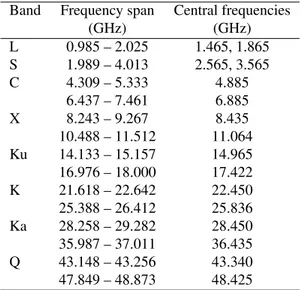
nized into 16 sub-bands, each of 128 MHz. The fre-quencies spanned are given in Table1. Only the data at frequencies above 20 GHz are used here; the lower frequency observations are discussed inStevens & Per-ley(2015). Because the observed sources are all fairly strong, there is no need to use the full bandwidth for the imaging; only a single 128 MHz-wide sub-band is needed. The center frequencies actually used to deter-mine the flux density and polarization of the sources are given in Table1.
The data were calibrated with the AIPS calibration package, using the regimen described byPerley & But-ler(2013a) as well as their revised flux density scale. The calibration took account of atmospheric opacity. Polarization calibration was established following the regimen described byPerley & Butler(2013b), includ-ing the adjusted position angles for 3C 286 described in that paper.
Accurate flux density measurements using the VLA require corrections for three factors which change the antenna gains. (1) Changes in electronic gains are monitored by injecting at 10 Hz a small amount of wideband noise into the receiver from a stable noise diode. This contributed power is detected by the cor-relator. Variations in this detected power are propor-tional to changes in the receiver gain, and are used to correct the visibilities for these changes. (2) Errors in antenna pointing are minimized by employing the referenced pointing technique, whereby the local an-tenna pointing offsets are determined using a nearby calibrator source, and the offsets are then employed for the target source. For this set of observations, all sources were strong enough to employ the technique directly. This reduced the typical pointing error from 10–20 arcsec to ∼ 5 arcsec. (3) Finally, variations in antenna gain with elevation are measured by fitting a second-order polynomial in elevation to the measure-ments of sources of known flux density during the ob-servations. There are typically 30 observations of such sources, over the full range of elevation available (typ-ically 10–80 degrees), permitting an estimate of the antenna gain as a function of elevation to better than 1%. At 28 GHz, the typical change in power gain of the VLA antennas is ∼ 10%. At 43 GHz, it can be as high as 30%.
Following these corrections, the flux density scale is set by observations of 3C 286, a source known to be stable over the past thirty years (Perley & Butler 2013a). At all frequencies above 10 GHz, the limit-ing factor in determinlimit-ing accurate flux densities with
the VLA are the residual pointing errors (seePerley & Butler 2013afor a fuller discussion).
Flux density determinations were made through di-rectly imaging the sources in Stokes parameters I, Q, and U, using well-established techniques for self-calibration and deconvolution (see Perley & Butler 2013afor details). The VLA resolution varied because of the the configuration employed as well as the dif-ferent declinations, δ, of the sources observed. Typ-ically, the resolution for the ’D’ configuration data is given by [60 × 60 csc(δ − 35◦)]/ν arcsec, with ν in gi-gahertz. For the second observing epoch, taken in a mixed configuration, the beam sizes are about half this size. The total flux density for a source was determined by integration of the source strength over an area en-compassing all visible emission. This approach was taken since the Planck beams were far larger than the VLA beams. While we also computed peak brightness for each source, we consistently used total flux densi-ties when making comparisons with Planck measure-ments. We also examined results in the visibility data to check for extended emission.
Any significant difference between total and peak brightness is an indication that the source may be re-solved. Clear evidence of resolution was found for several sources such as J2107+4213 (NGC 7027) and J0813+4812 (3C 196). In Section5.2, we discuss the effect of excluding evidently resolved sources.
The uncertainties in these VLA flux density mea-surements were determined from the scatter in the in-dividual observations of each source, as each object was typically observed five times during the course of each run. Potential systematic error in the flux den-sity scale introduced by Perley and Butler arises from uncertainties in the model for emission by Mars (the average dielectric constant of the surface; the extent of and changes in the polar caps, etc.) and in the transfer of measurements from Mars to 3C 286. These issues are discussed more fully in Perley & Butler(2013a), section 9. There, the estimated uncertainty in the flux density scale at 22 GHz is given as ∼ 2%, rising to ∼ 3% at 43 GHz.
3. ATCA Observations and Data Reduction 3.1. Observations
The Australia Telescope Compact Array (ATCA) observed the comparison sources between 2013 April 17 and 29, during the Planck observations described
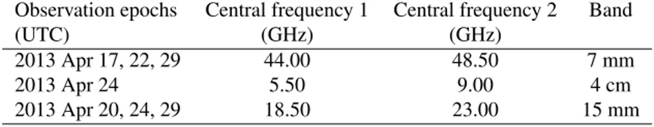
above (but days to weeks earlier than the VLA ob-servations). The Compact Array Broadband Back-end (CABB) system installed on ATCA (Wilson et al. 2011) provides two simultaneous sub-bands, each with 2048 MHz of bandwidth. On each day a different pair of simultaneous frequencies was observed, as detailed in Table2.
During each observing epoch, the sources were ob-served alternately for a few minutes at a time, so that each was observed over a range of hour angles and elevations. Since all of the sources had flux densi-ties above 100 mJy, integration time was not a pri-mary concern, and no source was observed for more than 25 min per epoch. Between scans on the target sources, a number of potential flux density calibrators were observed. These were the planets Venus, Mars, Uranus, and Neptune, and the gigahertz-peaked spec-trum (GPS) source PKS 1934−638; this latter source is regularly used as the primary flux density calibra-tor for the ATCA for frequencies below 25 GHz. To limit the effect of antenna gain changes as a function of elevation, the calibrator sources were observed over the same range of elevations as the program sources. For at least one measurement for each source at each epoch, the elevation of the calibrator source PKS 1934-638 matched the program sources to better than 2.65 degrees. The measured gains vary by less than 1% over such an elevation range for frequencies below 30 GHz, and by approximately 1% in the worst case for higher frequencies. We therefore conclude that our measure-ments are not biased by systematic elevation depen-dencies. The system temperature of each antenna was constantly monitored by injecting noise at the receiver front-end, and variations in system temperature were compensated for by scaling the amplitudes in the cor-relator.
The ATCA was in its H214 configuration during the observations. Five of the six ATCA antennas were separated by between 82 and 247 m. Observations were scheduled in this compact array to better match Planck’s resolution, to minimize possible resolution of complex sources, and to limit the effect of the atmo-sphere at the higher frequencies.
3.2. Data Reduction
All data reduction was done with the ATCA soft-ware reduction package Miriad (Sault et al. 2011). At the very beginning of the data reduction process, cor-rections for atmospheric opacity changes were made
using meteorological data recorded during the runs; the Miriad package uses the atmospheric models of Liebe (1985) to make these corrections. The gains derived through our calibration process displayed less than 3% variation over the range of zenith opacities ex-perienced during our observations, indicating that our opacity corrections were successful to at least that pre-cision. Elevation dependence of the gains was also cor-rected for at this stage.
3.2.1. Flux density model for PKS 1934−638 The Miriad software has a built-in model for the flux density of PKS 1934−638 as a function of fre-quency, based on the models ofReynolds(1994) and Sault(2003). In this paper, we use a new model for PKS 1934-638 which is derived by including mea-surements of its flux density at frequencies between 92 and 96 GHz. These high-frequency measurements were performed on 2012 August 12, with the ATCA in its H75 configuration. Only five of the six anten-nas were used due to receiver constraints. Observa-tions were made at night, in excellent, stable condi-tions. PKS 1934-638 was observed for a total of 63 minutes, and its flux density was measured by com-paring it to that observed for the planet Uranus, us-ing the de Pater (1990) model. Measurements were made in two independent 2048 MHz bands, centered at 93 GHz and 95 GHz. No opacity corrections were required during data reduction because atmospheric opacity changes are compensated for during the obser-vations through regular obserobser-vations of an absorbing paddle. Elevation-dependent gain changes were cor-rected for using the model ofSubrahmanyan (2002). In these observations, PKS 1934-638 covered the ele-vation range 32 to 44 degrees, while Uranus was ob-served at approximately 55 degrees elevation. The flux density of PKS 1934-638 was measured from the im-ages made in each band, and assigned to the central frequency of that band. Both images had a synthesized beam size of 7.70 x 5.17 arcseconds, and the flux den-sity was measured to be the same in each image, to within the uncertainties, at 0.11 ± 0.01 Jy. These flux densities, measured at such high frequency, are an ex-cellent constraint on the flux density model for PKS 1934-638.
We chose to modify the Sault (2003) flux den-sity model to incorporate these higher frequency flux density measurements, while assuming that the Sault (2003) model provides correct flux densities in the range 16 - 24 GHz. We make this assumption in
or-der that flux densities referenced against our modified model will closely match those made against theSault (2003) model, which has been in use for ATCA data reduction since 2003.
To do this, we first evaluated theSault(2003) model to get a list of the Stokes I flux density of PKS 1934-638 every 128 MHz between 10 GHz and 24 GHz. We assume a very conservative uncertainty of 0.1 Jy for each of these flux density values (slightly less than 10% uncertainty). The 93 GHz and 95 GHz measure-ments of PKS 1934-638, as listed above, are added to this list, and a first-order linear least-squares fit is made. The resulting flux density model fit is:
log S = 5.8870 − 1.3763 log ν, (1) where S is the flux density in Jy, ν is the frequency in MHz, and the log is base-10. This paper aims in part at evaluating how closely this proposed model agrees with the absolute calibration provided by Planck with-out making any other presumptions abwith-out the quality of the proposed model.
3.2.2. Calibration
For each observation, data from two independent 2048 MHz bands were independently reduced. Cali-bration began with the determination of the bandpass response and an initial estimate of the time-dependent gain variation of one of the stronger sources observed during that epoch. In the 4 cm band (4–11 GHz), PKS 1934−638 can be used for this purpose, since it is quite strong ( > 2 Jy) and its flux density model is known; thus, the bandpass determination should not need further correction.
At higher frequencies we used the strong VLBI calibrator B1921−293 to determine the bandpass re-sponse. Because Miriad does not have a model for the flux density of B1921−293, a flat (α = 0) spec-trum is the default during the bandpass determination. This is not entirely correct, but assuming that the actual flux density model has a power-law slope at these fre-quencies (an accurate assumption as it turns out) then a later correction for this slope is straightforward. This correction was done by transferring the bandpass so-lution to the flux density calibrator and then adjusting the bandpass slope to match the expected flux density behavior.
This flux calibrated bandpass solution was applied to all the other sources observed on the same day. The time-dependent gains were determined for each of the
other sources independently.
Once each source was self-calibrated in this way, the visibility plane data for all sources were rescaled to the bandpass calibrator’s flux density scale, and cor-rections were made for any slope variations introduced in the gain determination.
3.2.3. Measurements
Flux density measurements were made using Miriad from the vector-averaged spectra of each source. A first or second order linear least-squares fit was made to the observed Stokes I flux densities as a function of frequency over both of the simultaneously observed channels. The fit that best describes the spectra was used: this was determined by computing the rms of the residual amplitudes after the fitted model is subtracted from the spectra.
The ATCA did not observe the exact same bands as the VLA, so the fitted ATCA flux density models were evaluated at the VLA frequency that lay clos-est. The ATCA frequencies relevant for this paper are 17.422 GHz and 22.450 GHz in the 15 mm band, and 43.340 GHz and 48.425 GHz in the 7 mm band.
The Stokes I flux densities were the direct result of this process. The uncertainty for the Stokes I mea-surements is the rms scatter of the spectral amplitudes around the model fit.
3.2.4. Measurement Uncertainty
Since many of the comparison sources were ob-served in more than one of the seven epochs, we can look at the consistency of the measurements to get an estimate of the accuracy of our measurements. This es-timate will include any inconsistencies introduced by unrecognized variability of the sources.
In the 15 mm band we observed eight sources in two separate epochs, and in the 7 mm band we observed ten sources in two or more epochs, with seven observed in three epochs.
The observations of the eight multiply-observed sources in the 15 mm band show that on average, the Stokes I flux densities of these sources vary by 1.3% between the epochs, and by no more than 3.7%. In the 7 mm band, the average Stokes I variance is 5%, and the maximum variance is 10.7%. Since we cannot be certain that any of the sources varied intrinsically over the seven epochs, we have to assume conserva-tively that the actual measurement uncertainty could
be as large as 3.7% in the 15 mm band and 10.7% in the 7 mm band.
4. Planck Measurements
The Planck satellite (Tauber et al. 2010; Planck Collaboration I 2014) was launched on 2009 May 14, and scanned the sky stably and continuously from 2009 August 12 to 2013 October 23. Planck carried a scientific payload consisting of an array of 74 de-tectors sensitive to a range of frequencies between 25 and 1000 GHz, which scanned the sky simultaneously and continuously with an angular resolution vary-ing between 30 arcmin at the lowest frequencies and 5 arcmin at the highest. The array is arranged into two instruments. The detectors of the Low Frequency In-strument (Bersanelli et al. 2010;Mennella et al. 2011) are pseudo-correlation radiometers, covering three bands centered at 28.4, 44.1, and 70.4 GHz. The de-tectors of the High Frequency Instrument (Planck HFI Core Team 2011) are bolometers, covering six bands centered at 100, 143, 217, 353, 545, and 857 GHz. The design of Planck allows it to image the whole sky twice per year, with a combination of sensitivity, an-gular resolution and frequency coverage never before achieved.
For the results discussed here, flux densities at Planck’s three lowest frequencies were derived from special maps including only data taken during the pe-riod 2013 April 1 to 2013 June 30. These maps were constructed by the LFI Data Processing Cen-ter (DPC) in Trieste (Italy). Flux densities were de-rived using a non-blind approach at the position of each VLA or ATCA source using the Mexican Hat Wavelet 2 (MHW2) algorithm (Gonz´alez-Nuevo et al. 2006;L´opez-Caniego et al. 2006). This algorithm pre-serves the amplitudes of compact sources while greatly reducing the effects of large scale structure (such as Galactic foregrounds, a random background of faint sources or fluctuations in the CMB) as well as small scale fluctuations (such as instrument noise). Further details about the implementation of the MHW2 are given inPlanck Collaboration XXVI(2015).
For all but the strongest sources (or those in con-fused regions at low Galactic latitude), flux density uncertainties for individual sources were ∼0.15 Jy at 28 GHz and ∼0.26 Jy at 44 GHz.
The overall calibration uncertainty for the Planck LFI instrument at 30, 44, and 70 GHz was 0.35%, 0.26% and 0.20%, respectively (Planck Collaboration
II 2015). As noted in Section 1, the calibration is absolute in the sense that it is determined from the satellite’s orbital motion in the solar system (compared to the speed of light). It also depends on the abso-lute temperature of the cosmic microwave background, To = 2.7255 ± 0.0006K (Fixsen 2009), but the
uncer-tainty in that quantity is at the 0.02% level. 4.1. Beam Solid Angles
These special maps, like all Planck frequency maps, are presented in temperature units. To convert the mea-sured intensity of a source to flux density, we need to know the size of Planck’s effective beam: flux den-sity S ∝ Ω ∝ (FWHM)2, whereΩ is the entire solid
angle of the beam and FWHM is the full width at half maximum, derived fromΩ assuming a Gaussian beam for each receiver. Approximate values for each band are given in Table 3. These were derived from FEBeCoP beams (see Planck Collaboration IV 2015 andMitra et al. 2011) constructed for these maps; note that the beam shape and solid angle vary slightly from point to point in the sky. Extensive testing and cal-culations described inPlanck Collaboration IV(2014) give us confidence that we know Planck’s beam solid angle in the 30 GHz channel to a precision of ∼ 0.1%. The situation at 44 GHz is more complicated. Two of Planck’s three 44 GHz receiver-horn assemblies are lo-cated on one side of its focal plane, and at a substan-tial distance from its center (seePlanck Collaboration II 2011;Planck Collaboration IV 2015). As a conse-quence, the beams for these two horns are substantially elliptical and are broader than the beam for the third, which is located on the other side of the focal plane. The FWHM figure in Table3is a weighted average ac-curate to ∼ 0.2% (Planck Collaboration IV 2015). The weights used were the same as employed in the LFI mapmaking process (Planck Collaboration VI 2015).
In Section 5.1.2, we treat separately the two sets of horns, and the measurements derived from each. Note that the large separation of the 44 GHz horns also means that a given source is observed at two sepa-rate epochs as the Planck beams scan across the sky; the separation between the two 44 GHz observations is ∼ 6 days. We return to this issue in Section5where we consider the effects of variability in the flux density of these sources.
4.2. Color Correction and Frequency Interpola-tion of Planck Measurements
Since Planck’s calibration is based on the dipole signal induced in the CMB (which has a thermal spec-trum with flux density roughly ∝ ν2) but most of the
sources in this study have spectral indices α (Sν∝να) in a quite different range, 0 to −1, the Planck flux densities need to be color-corrected (seePlanck Col-laboration II 2015). This color correction, as well as the (small) interpolation from Planck band centers of 28.4 and 44.1 GHz to the standard VLA frequen-cies of 28.45 and 43.34 GHz, was made individually for each source at each frequency. The corrections were based on spectral indices derived from the very precise VLA measurements. To correct the 28 GHz data, we calculated the spectral index from flux den-sity measurements at 25.836 and 36.435 GHz, and at 44 GHz, we used the VLA measurements at 36.435 and 48.425 GHz. Typical values of these multiplicative corrections were 0.99–1.005 at 28 GHz and 0.98–1.00 at 44 GHz. For a given source, the color corrections and frequency interpolation can be made with a preci-sion of ∼ 0.1% or better. The color corrections tabu-lated inPlanck Collaboration II(2015), however, have an intrinsic uncertainty of up to 0.4% for the range of spectral indices we find. These uncertainties are in-cluded in our final error budget.
4.2.1. Extrapolation to VLA and ATCA Frequencies As listed in Section 3, the ATCA frequencies most closely overlapping Planck’s LFI bands were 22.45, 43.34, and 48.425 GHz. As for the VLA, the 43.34 GHz band was close to the Planck 44.1 GHz band center. Thus the color correction and extrapola-tion required for the Planck measurements were small, as noted above. As in the case of the VLA results, these corrections were made individually for each source, based on VLA spectral indices when available (and on ATCA 43.34 and 48.425 GHz measurements otherwise). Since the ATCA and VLA band centers match exactly, we included all 43.34 GHz observa-tions made at either instrument when we compare the results to extrapolated Planck measurements. In taking this step, we assume that the 43.34 GHz flux density scales at the VLA and ATCA are consistent (confirmed below in Section5.5).
We also also combined results from both ground-based instruments at 22.45 GHz. Comparing Planck observations with the VLA and ATCA results at
22.45 GHz, however, requires a much larger extrap-olation in frequency, again based on spectral indices determined from VLA or ATCA measurements. The color correction to some degree cancels the frequency extrapolation, but the overall adjustment required for Planckdata ranged from 0.7 to 1.3 (multiplicative). 4.3. Resulting Planck Measurements Interpolated
to Ground-Based Frequencies
The interpolated and color-corrected Planck flux densities, adjusted to match the frequencies of the ground-based observations, are given in columns 10, 11, and 13 of Table 4. The table also provides the approximate time intervals between Planck and VLA and/or ATCA observations. The tabulated Planck flux densities are averages over the entire three-month pe-riod. In some cases, sources were observed only once, over a period of a day or so; in other cases, especially for sources near the ecliptic poles, sources were ob-served for several days or more extended periods. In addition, as noted above, the 44 GHz measurements for each source occurred at two different epochs. We consider the effect of these complications further in Section5.
5. Comparison of Flux Densities
5.1. Planck vs. ground-based Flux Density Mea-surements
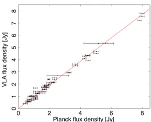
In Figures2,3 and4, we plot the fully corrected Planck flux densities against the corresponding VLA and ATCA measurements as described in Sections 2
and3. Not every VLA and ATCA source was detected by Planck. In some cases, this was because the source was too faint (as noted in Section1, sources were se-lected to cover a range of flux density). In other cases, at one or another of the Planck frequencies, the source fell just outside the area of the sky Planck scanned in the interval 2013 April 1 to June 30 (see Figure1). For sources that were observed in both early and late May at the VLA, we treat the two VLA measurements as independent, and plot both against the Planck results.
For each frequency, we also plot the best-fit linear relation. Since the Planck flux density errors domi-nated, and were roughly equal for most sources, we did not weight the data. In addition, we forced these fits to pass through (0, 0); these are referred to below as “constrained fits.” The consequences of this choice are discussed in Section5.3.1.
If the Planck and ground-based flux density scales agreed exactly, we would expect an exactly linear re-lation with unit slope. Measurement uncertainty in the Planckvalues (indicated by error bars in the figures), as well as source variability, produces the scatter seen in the figures.
5.1.1. Comparison of Planck with VLA Measure-ments at 28.45 GHz
Figure 2 shows the agreement between the cor-rected Planck and VLA measurements made at 28.45 GHz. The measured slope and the 1σ uncertainty of the relation are 0.964 ± 0.008, when the fit is con-strained to pass through (0, 0). This is changed to S(VLA)= 0.948S (Planck)+0.056 by allowing an un-constrained fit. We thus find that VLA flux densities run ∼ 4% (with a statistical scatter of ±0.8%) below the Planck measurements. This fit does not take into account any possible systematic errors in the Planck or ground-based measurements.
We next consider the potential systematic uncer-tainties in the Planck calibration, discussed in detail in Planck Collaboration III (2015). There are three sources of systematic error, which we assume are in-dependent. These include the uncertainty in the color correction mentioned above (taken as 0.4%); 0.06% uncertainty in the solid angle of the beam, taken from Planck Collaboration IV (2015); and 0.35% calibra-tion uncertainty, taken from Planck Collaboration II (2015). We combine these systematic errors in quadra-ture to arrive at an estimate of the systematic error. VLA flux densities run 3.6%±0.8%(stat)±0.5%(syst), or 3.6%±1.0% lower than those measured by Planck if we combine the two types of error in quadrature. This result is cited in Planck Collaboration XXVI(2015). Estimates of the systematic uncertainties in the VLA and ATCA flux densities are given in sections 2 and 3.2.4.
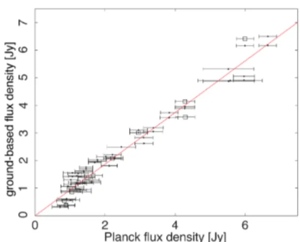
5.1.2. Comparison of Planck with VLA and ATCA Measurements at 22.45 GHz
As noted in Section4.2.1, comparing Planck mea-surements made at 28.45 GHz to VLA and ATCA val-ues at 22.45 GHz required a much larger extrapolation in frequency. This extrapolation (like the generally smaller color correction) made use of the spectral in-dex for each source. We employed several means of calculating spectral indices for each source. First, for those sources observed by the VLA, the spectral index
Fig. 2.— Comparison between color-corrected Planck and VLA measurements at 28.45 GHz; the observed scatter is due mainly to variability of the sources. The slope and 1σ uncertainty of the fit (solid line) are 0.964 ± 0.008.
could be found directly from 22.45 and 28.45 GHz ob-servations. For sources observed only at the ATCA, we calculated both a spectral index from 17 to 22 GHz and one from 22 to 43 GHz. For all but four of the sources involved, all the spectral indices agreed within errors, and we used an average for the extrapolation and color correction.
For the other four cases, we compared results us-ing the largest value for the derived spectral index for a given source with the results with the smallest value. This resulted in a ∼ 1σ shift in the overall slope. The results we adopted are based on taking that value for the spectral index of these 4 sources which produced the lowest scatter in the fit. As shown in Figure 3 , we find a slope of 0.967 ± 0.007(stat). In the case of the 22 GHz measurements, ground-based flux densi-ties again run low, but agree within the assumed ATCA and VLA uncertainties with the Planck values. 5.1.3. Comparison of Measurements at 43 GHz
Figure 4 demonstrates the agreement between the flux density scales used by Planck and by the two ground-based instruments at 43.34 GHz. The con-strained linear fit to all the data shows that the ground-based measurements are on average 6.2%±1.3% lower than Planck’s. Allowing an unconstrained fit gives S(ground based)= 0.933S (Planck)+0.018. While the
Fig. 3.— Color-corrected and extrapolated Planck flux densities compared to VLA measurements (dots) and ATCA measurements (open squares) of the same sources at 22.45 GHz; The slope and 1σ uncertainty of the fit (solid line) are 0.967 ± 0.007.
extrapolation from the Planck band center of 44.1 GHz to the VLA and ACTA frequency of 43.34 GHz is slightly larger than at 28.45 GHz, it is partially offset by the spectral-index dependent color correction. At 43.34 GHz, the overall uncertainty is dominated by the 1.3% statistical error in the slope of the fit, induced by Planckmeasurement errors and variability.
We estimate the systematic error as the quadrature sum of the uncertainty in the color correction (0.4%), the beam uncertainty < 0.2% (Planck Collaboration IV 2015), and the overall calibration < 0.26% (Planck Collaboration II 2015). We thus end with an ob-served difference in the flux density scales of 6.2% ± 1.3%(stat) ± 0.5%(syst); the ground-based measure-ments are fainter than Planck values by 6.2% ± 1.4%.
This discrepancy is much larger than either the color correction or the uncertainty in Planck’s beam solid angle, and also exceeds the quoted 3% accuracy of the flux density scale introduced byPerley & Butler (2013a). The discrepancy between Planck and ground-based flux densities is not significantly changed if we consider only the VLA measurements: if we omit the smaller number of ATCA measurements, the slope changes from 0.9384 to 0.9343.
Fig. 4.— Color-corrected (and extrapolated) Planck flux densities compared to VLA measurements (dots) and ATCA measurements (open squares) of the same sources at 43.34 GHz. The slope and 1σ uncertainty of the constrained fit (solid line) are 0.9384 ± 0.013.
5.1.4. Treating the 44 GHz Horns Separately To explore this discrepancy further, we also consid-ered separately the Planck measurements made with the single 44 GHz horn on one side of the focal plane, and measurements made by the two other horns on the other side of the focal plane. The separate mea-surements were noisier. We found a 1.7σ difference: the flux densities recorded by the single horn for these sources were on average 4.6% ± 2.7% higher. Even if we exclude all measurements made by this horn, how-ever, we still find that the remaining Planck measure-ments at 44 GHz run high compared to ground-based ones.
5.2. The Effect of Resolved Sources and Possible Confusion
The VLA beams have far smaller solid angles than Planck’s. As a consequence, four sources were heavily resolved by the VLA but not by Planck: J0813+4812 (3C 196), J1229+0203 (3C 273), J1411+5212 (3C 295) and J2107+4213 (the planetary nebula NGC 7027). Although in comparing measurements from the two instruments we always used the total VLA flux den-sity, which nominally corrects for resolution, we ex-amined the effect that dropping these four sources had on the slopes of the fit. If some flux were missed at the
VLA due to resolution, we would expect the slopes to increase slightly when dropping these sources. At 43.34 GHz, dropping these sources had only a small effect on the slope: it did increase slightly to 0.941 ± 0.013. At 28.45 GHz, the effect of dropping resolved sources was equally small, but in the oppo-site direction: the slope decreased to 0.958 ± 0.008. The same was true at 22.45 GHz: the slope changed to 0.963 ± 0.007.
We also investigated the possibility that Planck’s larger beam could incorporate radio sources other than the target source (loosely, ”confusion”). To first order, the Mexican Hat Wavelet 2 algorithm used to derive Planck’s flux densities corrects for a random distribu-tion of weak sources. In addidistribu-tion, we computed the probability of finding a weak source within Planck’s 32 arcminute beam at 28 GHz, employing 30 GHz source counts taken from Planck Collaboration XIII (2011). That probability falls below unity for sources with flux density > 10 mJy, which in turn is 2.5% or less of the flux density of even the weakest target sources we consider. At 44 GHz the counts (ibid) are lower and the beam solid angle is somewhat smaller, so the probability of finding a source > 10 mJy falls to 20%.
A referee pointed out that the distribution of ra-dio sources near our bright target sources might not be random. Radio sources, unlike dusty galaxies, are only weakly correlated – see, for example,Cress et al. (1996) – so our assumption of a random distribution is not unreasonable. Nevertheless, we performed a check by searching the NVSS catalog (Condon et al. 1998) for other sources within 10 arcmin of our tar-get sources. This catalog is constructed at 1.4 GHz a much lower frequency than we employed, but cov-ers much of the sky. Not surprisingly, given the well-established source counts at 1.4 GHz, we found a few weak sources around many of the target sources (the number ranged from 0 to 8). We also checked 20 ran-dom positions and found comparable numbers of weak sources in the same search area. Thus we found no in-dication of a significant increase in the number of weak radio sources near our bright target sources. Further-more, none of the weak sources except one near J1037-2934 had a measured 1.4 GHz flux density > 6% of the flux density of the target source in that search area. While the flux densities of most of these sources are unknown at the higher frequencies of Planck given typical synchrotron spectral indices, we expect them to be 4-30 times lower at 22 to 44 GHz. We end by
noting that in the particular case of J1037-2934, the Planckflux densities were observed to be slightly be-low, not above, the VLA values.
5.3. The Effect of Source Variability
Although we aimed to make the Planck and ground-based observations as close in time as possible, all the VLA observations were made at just two epochs in May, and the ATCA observations ended in late April. As columns 14 and 15 of Table 4 show, the inter-vals between ground and space-based measurements ranged from less than a day to 45 days as a conse-quence. Since many of our sources are AGN (includ-ing many blazars) we expect them to vary. Variability will introduce scatter into our plots, but should not in principle bias them.
5.3.1. Possible effects of bias
One could argue, however, that some form of selec-tion bias would make it less likely for Planck to de-tect marginal sources when they happen to be in their low luminosity states, thus artificially boosting the av-erage Planck flux densities at the faint end. Indeed, there is evidence in Figure4 that the 44 GHz Planck measurements at the faint end may be subject to an ef-fect that biases the Planck flux density measurements high for the faintest sources (see the detailed discus-sion in Crawford et al. 2010). We reduce the im-pact of this effect by forcing the fits to pass through (0, 0). We also made a trial of dropping all 44 GHz sources with Planck flux densities < 1.4 Jy. The re-sult was to shift the slope of the constrained fit slightly to 0.943 ± 0.013. The unconstrained fit to the strong (S > 1.4 Jy) 44 GHz sources has a much flatter slope of 0.87. Bias in the flux densities of weak sources is evidently not responsible for the discrepancy between Planck and ground-based measurements at 43 GHz. The closer spacing in time of the ATCA observations made such a test less useful for those data.
5.3.2. Dropping known variable or resolved sources As one way of assessing the effect of source vari-ability on our comparisons, we looked first at the sources (about half the sample) observed twice at the VLA, once in early May and once at the end of the month. At 43 GHz, five sources changed observed flux density by more than ∼ 6% over that interval: J0813+4812 (resolved), J0958+6533, J1037−2914, J2107+4213 (NGC 7027, resolved), and J2146−1525.
In addition, J0854+2006 and J1849+6705 varied at 28 GHz. Note that two of these apparently ”variable” sources J0813+4812 and J2107+4213 are among the four resolved sources discussed in Section5.2above. Although we always employed total flux densities, the apparent change in VLA flux density of the two heav-ily resolved sources is certainly in large part due to the different beam solid angles resulting from the dif-ferent configurations used in early and late May. At 43.34 GHz, as these variable sources were dropped one by one, the slope settled to 0.941±0.013. As expected, variability introduces scatter but no significant bias in the fits. J2253+1608 = 3C 454.3 is a special case. While the observed change in flux density between the two epochs of the VLA observations happened to be small at all frequencies, the source clearly did vary during the (longer) Planck mission (Planck Collabo-ration XV 2011). VLA and Planck measurements at 43 GHz differ by 15–18%. If we also drop this source on grounds of assumed variability, the derived slope at 43 GHz moves to 0.958 ± 0.013, a ∼ 1.5σ change.
Thus dropping variable and/or resolved sources re-duces, but does not eliminate, the discrepancy between Planckand ground-based flux densities at 43 GHz.
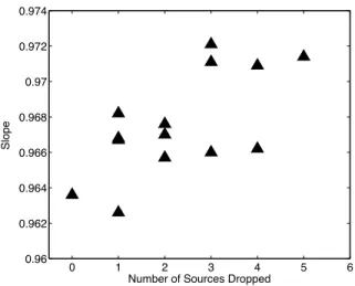
In contrast, a more systematic change was found at 28.45 GHz as variable sources (five in this case) were dropped one by one. In Figure 5, we show the re-sult of dropping more and more sources (in various orders): the slope averaged to 0.97 ± 0.0075. Again, J2253+1608 had a particularly large effect; also drop-ping just that source produced a ∼ 1σ change in the slope to 0.977 ± 0.0075. On the other hand, dropping variable and/or resolved sources had little effect on the 22 GHz data: the slope remained in the range 0.963 to 0.972.
5.3.3. Restricting the allowed time interval between Planck and ground-based observations We also tried restricting the fits to sources observed by Planck within one week of one of the VLA or ATCA runs. That left only about half of the data. As expected, this restriction reduced the scatter in the plots of ground-based vs. Planck flux density. At 28.45 GHz, the slope changed by approximately 1σ to 0.980 ± 0.009. At 43.34 GHz, the same restric-tion led to a change in slope from 0.9384 ± 0.013 to 0.940±0.012 (note that the uncertainty barely changed even though we retained only about half the data, be-cause the scatter in the data induced by variability was
0 1 2 3 4 5 6 0.96 0.962 0.964 0.966 0.968 0.97 0.972 0.974
Number of Sources Dropped
Slope
Fig. 5.— Change in the slope of the constrained fits of the 28.45 GHz data as more and more variable sources are dropped (in various orders); note that the resulting change is smaller than or comparable to the statistical uncertainty in the slope of ±0.008, and that the slope settles to ∼ 0.97.
reduced).
Given these results, we conclude that variability does not alter the overall conclusion that the ground-based flux density scales run below those established by Planck. The ground-based flux densities run roughly 3% below the Planck flux densities at 22 and 28 GHz, and 5–6% below them at 43 GHz.
5.4. The Effect of Color Corrections
As noted in Section4.2, the Planck data needed to be color corrected as well as interpolated to match the VLA and ATCA central frequencies. We performed two tests on the effect of the small color corrections made to the Planck data. First, we compared the uncorrected Planck observations in the 30 GHz band to the VLA results. Omitting the color corrections changed the observed slope from 0.964 to 0.968. We also separated the Planck data into two parts, one hav-ing a very small (1.000 ± 0.005) color correction, the other with a larger and more spectral-index-dependent color correction. The difference in the resulting fits to VLA data was at the 0.1σ level.
5.5. Comparison of VLA and ATCA Flux Density Scales at 43.34 GHz
We turn next to a direct comparison of flux density scales employed by the two major interferometric ar-rays, the VLA in the north and the ATCA in the south. We note that questions have been raised (see Sajina et al. 2011) about the agreement of calibration scales at 22 GHz, before the recent re-estimates of flux den-sity scales described in Sections 2 and 3 above. These direct comparisons between the new Perley-Butler and the new Stevens scales are treated inStevens & Perley (2015) and cover a much wider range of frequencies than those considered here, as well as a wider range of flux density. Since we have combined 43.34 GHz observations by the two instruments when making the comparison to Planck, however, we need to be certain that the flux density scales used at the two interferom-eters agree at that frequency. We checked this by di-rectly comparing VLA and ATCA measurements for 14 sources observed in common at 43.34 GHz: on av-erage, VLA measurements were 0.990±0.011 those of ATCA measurements of the same source – at the high-est frequencies, the new Perley-Butler and Stevens flux density scales agree well.
5.6. Best estimates of VLA–Planck flux density comparison
We summarize this section by giving our best es-timates of the small difference between flux densi-ties observed by Planck and the ground-based instru-ments. We take account of source variability as dis-cussed in Section 5.3. At 28.45 GHz, we find that VLA flux densities are lower than Planck’s by 2–3% with a combined systematic and statistical error of 1%. At 22.45 GHz, ATCA and VLA flux densities are 3– 3.5% lower than Planck’s, again with a combined er-ror of ∼ 1%. At 43.34 GHz, on the other hand, the discrepancy is larger: Planck flux densities are higher by 5–6% than those from either ground-based instru-ment, with a combined systematic and statistical er-ror of 1.4%. At both 28.45 and 43.34 GHz, these re-sults are consistent with, but more precise than, the values based on a less complete analysis of these data inPlanck Collaboration XXVI(2015).
6. Polarization
We attempted to compare Planck measurements of polarized flux density with those obtained at the VLA and ACTA. Very few of the sources observed in this
program had enough polarized flux to be robustly de-tected by Planck. One of these was 3C 273. The Planck30 GHz polarized flux density (color-corrected and extrapolated to 28.45 GHz for comparison with the VLA) was 835 ± 70 mJy, while the VLA observed 813 ± 70 mJy. At 43.34 GHz the Planck polarized flux density was 567 ± 97 mJy, as compared with 623 ± 70 mJy seen by the VLA. At both frequencies, the mea-sured polarization angles agreed to ±2◦. Further re-finements of the Planck polarization measurements are planned, including more scrutiny of the possible leak-age of total power into polarization. At this point, we simply report that there are no evident discrepancies between the Planck and ground-based polarization. 7. Summary and Discussion
In conclusion, we see that the comparison of Planck data with VLA data at 28.45 GHz yields acceptable agreement: the VLA data run on average 2–3% fainter than Planck’s, which is within the margin of error of the VLA flux density scale. Similarly, the Planck 28.45 GHz data that have been extrapolated and com-pared to the VLA and ATCA data at 22.45 GHz are about 3 − 3.5% higher than the ground-based measure-ments, which is just within the margin of statistical and systematic error. The more problematic compar-ison is that between Planck 44.1 GHz data (extrapo-lated to 43.34 GHz) and the ground-based instruments at 43.34 GHz. Planck data were consistently 5–6% higher than the ground-based measurements. This re-mained largely unchanged when the Planck data were compared with the VLA and ATCA individually, when the two sets of 44 GHz Planck horns were compared separately to the ground-based instruments, when four resolved sources from the VLA data were dropped, and when variable sources were dropped (individu-ally and in all combinations). We suggest therefore that the difference in flux measurements in the 43 GHz range results from a difference in calibration. This discrepancy could affect precision flux density com-parisons between instruments, and would also affect source spectra that included 43 GHz data.
We end by asking whether the difference in flux density scales we have demonstrated could be due to a calibration mismatch between Planck and WMAP, since the VLA flux density scale is based on the WMAP calibration. Planck–WMAP calibration has been examined in detail in Planck Collaboration II (2015) and Planck Collaboration V (2015) for the
Planckbands considered here. Following the initial re-lease of Planck data in 2013, there was a small upward adjustment of the Planck calibration (which brings it closer to the WMAP calibration). The shifts were +0.45% and +0.64% at 28 and 44 GHz, respectively. Even with these slight shifts, the WMAP calibration remains ∼ 1% higher than Planck’s, so the difference is unlikely to explain why the VLA flux densities ap-pear to be a bit low. It is important to note, however, that the comparison of Planck and WMAP calibration is based on observations of the CMB (both the dipole and CMB fluctuations at degree scales). These have a different spectrum than the radio sources considered here, and have larger angular scales. A better com-parison is between Planck and WMAP observations of planets (essentially point sources for both instru-ments). Measurements of Jupiter are compared in Planck Collaboration V (2015). These indicate that Planck’s measurements of the brightness temperature of Jupiter agree with WMAP’s to 0.2±1.0% at 28 GHz, and ∼ 0.0 ± 1% at 44 GHz. Thus we currently have no convincing explanation for the observed discrepancy. We can speculate on possible contributing factors: er-rors in the model for secular changes in the emission of Mars, or in corrections for atmospheric absorption, or in the beam solid angles of one of the satellite ex-periments. Further refinements of the Planck data and analysis, expected in the next year, may allow us to check the last of these.
We are deeply indebted to Kris Gorski, Sanjit Mi-tra, and Luca Pagano of the FEBeCoP team who helped in the construction of the beams used to de-rive flux densities from the Planck maps. The dates that Planck observed each source were supplied by Jonathan Leon Tavares, then at Aalto University, Fin-land. MLC acknowledges the Spanish MINECO Projects AYA2012-39475-C02-01 and Consolider-Ingenio 2010 CSD2010-00064. The Planck Collab-oration acknowledges the support of: ESA; CNES and CNRS/INSU-IN2P3-INP (France); ASI, CNR, and INAF (Italy); NASA and DoE (USA); STFC and UKSA (UK); CSIC, MINECO, JA, and RES (Spain); Tekes, AoF, and CSC (Finland); DLR and MPG(Germany); CSA (Canada); DTU Space (Den-mark); SER/SSO (Switzerland); RCN (Norway); SFI (Ireland); FCT/MCTES (Portugal); ERC and PRACE (EU). A description of the Planck Collaboration and a list of its members, indicating which technical or scientific activities they have been involved in, can be
found at http: //www.cosmos.esa.int/web/planck/planck-collaboration.
Facilities:ATCA, Planck, VLA REFERENCES
Baars, J. W. M., Genzel, R., Pauliny-Toth, I. I. K., & Witzel, A. 1977, A&A, 61, 99
Bersanelli, M., Mandolesi, N., Butler, R. C., et al. 2010, A&A, 520, A4
Condon, J. J., Cotton, W. D., Greisen, E. W., et al. 1998, AJ, 115, 1693
Crawford, T. M., Switzer, E. R., Holzapfel, W. L., et al. 2010, ApJ, 718, 513
Cress, C. M., Helfand, D. J., Becker, R. H., Gregg, M. D., & White, R. L. 1996, ApJ, 473, 7
de Pater, I. 1990, ARA&A, 28, 347 Fixsen, D. J. 2009, ApJ, 707, 916
Gonz´alez-Nuevo, J., Arg¨ueso, F., L´opez-Caniego, M., et al. 2006, MNRAS, 369, 1603
Hafez, Y. A., Davies, R. D., Davis, R. J., et al. 2008, MNRAS, 388, 1775
Hinshaw, G., Weiland, J. L., Hill, R. S., et al. 2009, ApJS, 180, 225
Liebe, H. J. 1985, Radio Science, 20, 1069
L´opez-Caniego, M., Herranz, D., Gonz´alez-Nuevo, J., et al. 2006, MNRAS, 370, 2047
Massardi, M., & Burigana, C. 2010, New A, 15, 678 Mennella, A., Butler, R. C., Curto, A., et al. 2011,
A&A, 536, A3
Mitra, S., Rocha, G., G´orski, K. M., et al. 2011, ApJS, 193, 5
Perley, R. A., & Butler, B. J. 2013a, ApJS, 204, 19 —. 2013b, ApJS, 206, 16
Planck HFI Core Team. 2011, A&A, 536, A4 Planck Collaboration I. 2011, A&A, 536, A1 Planck Collaboration II. 2011, A&A, 536, A2 Planck Collaboration XIII. 2011, A&A, 536, A13
Planck Collaboration XV. 2011, A&A, 536, A15 Planck Collaboration I. 2014, A&A, 571, A1 Planck Collaboration IV. 2014, A&A, 571, A4 Planck Collaboration I. 2015, A&A, submitted,
arXiv:1502.01582
Planck Collaboration II. 2015, A&A, submitted, arXiv:1502.01583
Planck Collaboration III. 2015, A&A, submitted Planck Collaboration IV. 2015, A&A, submitted,
arXiv:1502.01584
Planck Collaboration V. 2015, A&A, submitted, arXiv:1505.08022
Planck Collaboration VI. 2015, A&A, submitted, arXiv:1502.01585
Planck Collaboration XXVI. 2015, A&A, submitted, arXiv:1507.02058
Reynolds, J. 1994, ATNF Memo Series 39.3/040 Sajina, A., Partridge, B., Evans, T., et al. 2011, ApJ,
732, 45
Sault, R. J. 2003, ATNF Memo Series AT/39.3/124 Sault, R. J., Teuben, P. J., & Wright, M. C. H.
2011, MIRIAD: Multi-channel Image Reconstruc-tion, Image Analysis, and Display, astrophysics Source Code Library, ascl:1106.007
Stevens, J., & Perley, R. 2015, in preparation
Subrahmanyan, R. 2002, ATNF Memo Series AT39.3/117
Tauber, J. A., Mandolesi, N., Puget, J., et al. 2010, A&A, 520, A1
Weiland, J. L., Odegard, N., Hill, R. S., et al. 2011, ApJS, 192, 19
Wilson, W. E., Ferris, R. H., Axtens, P., et al. 2011, MNRAS, 416, 832
This 2-column preprint was prepared with the AAS LATEX macros
v5.2.
Table 1: Frequencies employed at the VLA. Band Frequency span Central frequencies
(GHz) (GHz) L 0.985 – 2.025 1.465, 1.865 S 1.989 – 4.013 2.565, 3.565 C 4.309 – 5.333 4.885 6.437 – 7.461 6.885 X 8.243 – 9.267 8.435 10.488 – 11.512 11.064 Ku 14.133 – 15.157 14.965 16.976 – 18.000 17.422 K 21.618 – 22.642 22.450 25.388 – 26.412 25.836 Ka 28.258 – 29.282 28.450 35.987 – 37.011 36.435 Q 43.148 – 43.256 43.340 47.849 – 48.873 48.425
Table 2: Frequencies employed at ATCA.
Observation epochs Central frequency 1 Central frequency 2 Band
(UTC) (GHz) (GHz)
2013 Apr 17, 22, 29 44.00 48.50 7 mm
2013 Apr 24 5.50 9.00 4 cm
2013 Apr 20, 24, 29 18.50 23.00 15 mm
Table 3: Planck characteristics.
Band Band Center Frequency Beam FWHM
(GHz) (arcmin)
30 28.4 32
44 44.1 27
Table 4 Flux D ensity M easurements 1 2 3 4 5 6 7 8 9 10 11 12 13 14 15 VLA VLA VLA VLA VLA VLA A TCA A TCA Planck Planck Planck Planck Planck T ime Gap T ime Gap Source 22.450 25.836 28.450 36.435 43.340 48.425 22.45 43.34 Ra w 28 Corr . 28 Corr . 22 Ra w 44 Corr 43 30 GHz 44 GHz J0725 − 0054 5.4412 5.3963 5.3553 5.2238 4.9889 4.9017 .. . .. . 5.6118 5.6138 5.7801 .. . .. . 28 .. . J0745 − 0044 1.3696 1.2990 1.2463 1.1203 1.0332 0.9863 .. . .. . 1.241 1.2387 1.3651 .. . .. . 22 21 .. . .. . .. . .. . .. . .. . .. . 1.0190 1.241 .. . 1.3656 .. . .. . 19 18 B0754 + 100 .. . .. . .. . .. . .. . .. . 1.0680 0.9200 0.8897 .. . 0.8913 1.2336 1.22 82 6 11 J0813 + 4812 0.7266 0.6345 0.5461 0.3995 0.3064 0.2546 .. . .. . 0.6356 0.6289 0.8326 0.7133 0.7180 44 20 0.7452 0.6243 0.5592 0.4043 0.3365 0.2 801 .. . .. . 0.6356 0.6295 0.8326 0.7133 0.7166 18 .. . J0826 − 2230 1.3345 1.3029 1.2601 1.2051 1.1611 1.1342 .. . .. . 1.5763 1.5758 1.6708 1.2537 1.2482 3 14 .. . .. . .. . .. . .. . .. . 1.3190 1.2130 1.5763 .. . 1.6708 1.2537 1.2470 .. . 1 B0826 − 373 .. . .. . .. . .. . .. . .. . 1.2360 0.8600 0.9241 .. . 1.0399 1.0575 1.056 0 .. . .. . B0829 + 046 .. . .. . .. . .. . .. . .. . 0.5740 0.5420 0.5147 .. . 0.5203 0.8488 0.844 2 3 1 B0834 − 201 .. . .. . .. . .. . .. . .. . 1.7180 1.2980 1.8841 .. . 2.0921 1.6113 1.607 5 .. . 1 J0854 + 2006 3.9721 4.0049 3.9266 3.8965 3.8849 3.9594 .. . .. . 4.5059 4.5075 4.5509 4.3026 4.2730 27 27 4.5606 4.4371 4.3473 4.1311 3.9458 3.89 57 .. . .. . 4.5059 4.5039 4.7311 4.3026 4.2838 1 1 .. . .. . .. . .. . .. . .. . 4.5030 4.1350 4.5059 .. . 4.5008 4.3026 4.2795 8 2 .. . .. . .. . .. . .. . .. . 4.5030 3.5740 4.5059 .. . 4.5277 4.3026 4.2902 8 14 J0900 − 2808 0.5523 0.5263 0.5080 0.4552 0.3936 0.3698 .. . .. . .. . .. . .. . .. . .. . .. . 11 .. . .. . .. . .. . .. . .. . .. . 0.4080 .. . .. . .. . .. . .. . .. . .. . J0909 + 0121 2.0568 2.1213 2.1504 2.1301 2.0977 2.0489 .. . .. . 2.2373 2.2394 2.0806 2.2785 2.2674 17 1 1.9910 2.0569 2.1077 2.1124 2.0615 2.002 1 .. . .. . 2.2373 2.2399 2.0247 2.2785 2.2685 1 .. . J0920 + 4441 1.3263 1.3010 1.2477 1.1419 1.0669 1.0525 .. . .. . 1.1352 1.1339 1.2089 0.9517 0.9485 25 1 1.3150 1.2583 1.2473 1.1183 1.0637 0.986 3 .. . .. . 1.1352 1.1339 1.1976 0.9517 0.9499 1 .. . J0927 + 3902 8.1303 7.7399 7.5306 6.8295 6.1684 5.9942 .. . .. . 7.9907 7.9816 8.6299 6.6606 6.6481 22 1 8.3966 7.9208 7.8075 7.0650 6.4944 6.053 6 .. . .. . 7.9907 7.9824 8.6299 6.6606 6.6514 1 .. . J0927 − 2034 2.0287 2.0854 1.9939 1.8813 1.8093 1.6940 .. . .. . 1.9514 1.9500 2.0099 2.1300 2.1239 2 3 1.9501 1.9466 1.9256 1.8807 1.8155 1.767 4 .. . .. . 1.9514 1.9507 2.0099 2.1300 2.1207 10 .. . J0948 + 4039 0.8293 0.7814 0.7433 0.6495 0.5917 0.5473 .. . .. . 1.1227 1.1202 1.2574 0.9040 0.9037 17 1 0.8708 0.8103 0.7767 0.6831 0.6150 0.575 0 .. . .. . 1.1227 1.1203 1.2574 0.9040 0.9037 2 .. . J0956 + 2515 1.4862 1.5538 1.5868 1.6306 1.6225 1.7411 .. . .. . 1.6787 1.6808 1.5024 1.4048 1.3916 6 9 1.4884 1.5178 1.5456 1.5740 1.5744 1.579 0 .. . .. . 1.6787 1.6808 1.5779 1.4048 1.3959 9 .. . J0958 + 6533 1.2091 1.2440 1.2564 1.2638 1.3060 1.2690 .. . .. . 1.2575 1.2586 1.1820 1.0302 1.0236 27 1 1.2118 1.1983 1.2069 1.1726 1.1414 1.108 5 .. . .. . 1.2575 1.2584 1.2575 1.0302 1.0257 2 .. . J1037 − 2934 1.4619 1.4299 1.3915 1.2539 1.2015 1.1026 .. . .. . 1.1202 1.1187 1.1762 1.1931 1.1909 .. . .. . 1.7056 1.6865 1.6775 1.5661 1.4445 1.395 5 .. . .. . 1.1202 1.1202 1.1426 1.1931 1.1903 .. . .. . J1044 + 8054 1.0657 1.0212 1.0067 0.9262 0.8760 0.8420 .. . .. . 0.8271 0.8265 0.8767 .. . .. . .. . .. . 1.0851 1.0557 1.0543 0.9901 0.9279 0.887 6 .. . .. . 0.8271 0.8270 0.8477 .. . .. . .. . .. . J1048 + 7143 1.8504 1.8296 1.8064 1.7218 1.6938 1.6419 .. . .. . 1.7089 1.7087 1.7430 1.4655 1.4584 24 13 1.9063 1.8779 1.8911 1.8215 1.7574 1.695 4 .. . .. . 1.7089 1.7098 1.7259 1.4655 1.4598 1 .. . J1048 − 1909 1.8979 1.8446 1.7597 1.5760 1.4246 1.4053 .. . .. . 1.8368 1.8332 1.9837 1.0704 1.0679 .. . .. . 1.9657 1.9098 1.9078 1.7110 1.5557 1.486 3 .. . .. . 1.8368 1.8356 1.8919 1.0704 1.0689 .. . .. . J1104 + 3812 0.6433 0.6400 0.6384 0.6364 0.6349 0.6275 .. . .. . 0.8833 0.8841 0.8921 .. . .. . .. . .. . J1130 + 3815 1.1229 1.0702 1.0232 0.9357 0.8961 0.8480 .. . .. . 1.1205 1.1188 1.2325 0.9896 0.9863 6 6 J1153 + 8058 0.8303 0.7782 0.7569 0.6641 0.6048 0.5600 .. . .. . 0.687 0.6857 0.7557 .. . .. . 32 6
Table 4— Continued 1 2 3 4 5 6 7 8 9 10 11 12 13 14 15 VLA VLA VLA VLA VLA VLA A TCA A TCA Planck Planck Planck Planck Planck T ime Gap T ime Gap Source 22.450 25.836 28.450 36.435 43.340 48.425 22.45 43.34 Ra w 28 Corr . 28 Corr . 22 Ra w 44 Corr 43 30 GHz 44 GHz 0.8424 0.7940 0.7659 0.6733 0.6120 0.5691 .. . .. . 0.687 0.6857 0.7557 .. . .. . 6 .. . J1229 + 0203 .. . 17.5000 16.9000 15.1000 1 4.6000 13.3000 .. . .. . .. . .. . .. . 10.5181 .. . .. . .. . J1331 + 3030 2.5063 2.2582 2.1018 1.7465 1.5331 1.4103 .. . .. . 2.1662 2.1573 2.5561 1.2300 1.2314 .. . .. . 2.5063 2.2582 2.1018 1.7465 1.5331 1.4103 .. . .. . 2.1662 2.1573 2.5561 1.2300 1.2314 .. . .. . J1411 + 5212 0.9449 0.7924 0.7006 0.5035 0.4119 0.3398 .. . .. . 0.8422 0.8333 1.1159 .. . .. . .. . .. . 0.9546 0.7868 0.6977 0.4941 0.3985 0.3324 .. . .. . 0.8422 0.8334 1.1369 .. . .. . .. . .. . J1642 + 6856 2.5780 2.4221 2.3904 2.0806 1.9259 1.7792 .. . .. . 2.3308 2.3268 2.5172 1.7068 1.7053 1 12 2.7235 2.5418 2.5054 2.1874 1.9503 1.8048 .. . .. . 2.3308 2.3268 2.5172 1.7068 1.7062 8 .. . J1716 + 6836 0.5135 0.4996 0.5121 0.4865 0.4812 0.4581 .. . .. . 0.5626 0.5630 0.5626 .. . .. . .. . 45 J1748 + 7005 0.7770 0.7648 0.7783 0.7504 0.7474 0.7167 .. . .. . 0.9569 0.9576 0.9569 .. . .. . 3 .. . J1800 + 7828 2.4772 2.4091 2.3748 2.2463 2.1831 2.1160 .. . .. . 1.9562 1.9559 2.0442 .. . .. . 35 12 2.4732 2.4277 2.4050 2.2741 2.1687 2.0830 .. . .. . 1.9562 1.9559 2.0148 .. . .. . 9 .. . J1806 + 6949 1.3699 1.3559 1.3720 1.3372 1.2859 1.2530 .. . .. . 1.3775 1.3795 1.3775 .. . .. . 3 3 1.3910 1.3600 1.3772 1.3491 1.2831 1.2318 .. . .. . 1.3775 1.3795 1.3912 .. . .. . 8 .. . J1842 + 6809 0.5496 0.5823 0.6199 0.6549 0.6731 0.6656 .. . .. . 0.5875 0.5889 0.4670 .. . .. . 7 6 J1849 + 6705 1.8407 1.8476 1.8987 1.8755 1.8445 1.8163 .. . .. . 1.8643 1.8664 1.7710 .. . .. . 1 6 1.6832 1.6823 1.7237 1.7140 1.6826 1.6451 .. . .. . 1.8643 1.8664 1.7897 .. . .. . 4 .. . J1911 − 2007 1.9472 2.0366 2.1018 2.1430 2.1451 2.1244 .. . .. . 1.9803 1.9836 1.7228 2.0381 2.0251 20 30 J1924 − 2914 7.8316 7.4155 7.2218 6.6232 6.1598 5.9570 .. . .. . 7.8556 7.8490 8.5233 6.0125 5.9952 27 27 .. . .. . .. . .. . .. . .. . 8.3900 6.4100 7.8556 .. . 8.6055 6.0125 5.9982 12 12 J1927 + 6117 1.0695 1.0348 1.0159 0.9370 0.8856 0.8344 .. . .. . 1.1052 1.1044 1.1604 .. . .. . 4 7 B1933 − 400 .. . .. . .. . .. . .. . .. . 1.0510 0.9380 0.9022 .. . 0.9025 .. . .. . 14 1 B1954 − 388 .. . .. . .. . .. . .. . .. . 1.5410 1.4580 1.5114 .. . 1.5277 1.6823 1.6724 6 3 J1955 + 3151 1.2507 1.2283 1.2374 1.1631 1.1208 1.0563 .. . .. . 1.2043 1.2046 1.2163 .. . .. . 1 .. . J2000 − 1749 1.4553 1.6133 1.7424 2.0582 2.2130 2.3295 .. . .. . 1.6514 1.6558 1.1549 2.2405 2.2150 6 .. . .. . .. . .. . .. . .. . .. . 1.4610 2.0730 1.651 4 .. . 1.2828 2.2405 2.2117 9 .. . J2011 − 1546 1.8644 1.7810 1.7287 1.5680 1.4091 1.3512 .. . .. . 1.6371 1.6351 1.7598 1.4762 1.4742 11 2 .. . .. . .. . .. . .. . .. . 1.9530 1.3900 1.637 1 .. . 1.7598 1.4762 1.4742 1 8 J2015 + 3710 4.4837 4.5687 4.6839 4.8017 4.8964 4.7478 .. . .. . .. . .. . .. . 5.6103 5.5 774 2 .. . J2025 + 3342 2.7372 2.6677 2.6865 2.6282 2.4944 2.3788 .. . .. . 2.5418 2.5437 2.5799 2.4773 2.468 9 5 .. . J2035 + 1056 0.3662 0.3724 0.3935 0.4195 0.4420 0.4350 .. . .. . 0.4298 0.4308 0.3782 .. . .. . .. . .. . 0.3721 0.3854 0.3953 0.4122 0.4408 0.4606 .. . .. . 0.4298 0.4307 0.3868 .. . .. . .. . .. . .. . .. . .. . .. . .. . .. . 0.3970 0.4560 0.4 298 .. . 0.3938 .. . .. . .. . .. . B2047 + 039 .. . .. . .. . .. . .. . .. . 0.4900 0.3690 0.6028 .. . 0.6633 0.8853 0.8832 15 12 J2101 + 0341 0.9552 0.9669 0.9999 1.0220 1.0348 1.0104 .. . .. . 0.9398 0.9415 0.8646 1.1644 1.1 576 5 6 0.9673 0.9776 0.9844 0.9809 0.9702 0.9379 .. . .. . 0.9398 0.9407 0.9160 1.1644 1.1587 10 .. . B2106 − 413 .. . .. . .. . .. . .. . .. . 0.5790 0.3860 0.8273 .. . 0.9475 0.8923 0.8920 11 10 J2107 + 4213 5.3846 5.2969 5.3540 5.1841 5.3145 5.0319 .. . .. . 5.1875 5.1909 5.2134 5.5505 5.5207 .. . .. . 5.4373 5.3228 5.3061 5.1025 4.8688 4.6650 .. . .. . 5.1875 5.1893 5.3171 5.5505 5.5318 .. . .. . J2123 + 0535 1.0483 0.9933 0.9814 0.9092 0.8821 0.8390 .. . .. . 0.7480 0.7477 0.7966 .. . .. . 4 7 1.0384 0.9820 0.9480 0.8631 0.8187 0.7782 .. . .. . 0.7480 0.7470 0.8190 .. . .. . 18 .. . J2129 − 1538 0.6833 0.6052 0.5562 0.4366 0.3769 0.3304 .. . .. . .. . .. . .. . .. . .. . .. . .. .
Table 4— Continued 1 2 3 4 5 6 7 8 9 10 11 12 13 14 15 VLA VLA VLA VLA VLA VLA A TCA A TCA Planck Planck Planck Planck Planck T ime Gap T ime Gap Source 22.450 25.836 28.450 36.435 43.340 48.425 22.45 43.34 Ra w 28 Corr . 28 Corr . 22 Ra w 44 Corr 43 30 GHz 44 GHz .. . .. . .. . .. . .. . .. . 0.7000 0.3690 .. . .. . .. . .. . .. . .. . .. . J2130 + 0502 0.4797 0.4120 0.3819 0.2928 0.2391 0.2075 .. . .. . 0.4533 0.4502 0.5646 .. . .. . 2 .. . J2131 − 1207 1.4891 1.4109 1.3779 1.2916 1.2447 1.2199 .. . .. . 1.6550 1.6541 1.7791 1.6187 1.6116 1 10 1.4631 1.3949 1.3654 1.2591 1.1926 1.1145 .. . .. . 1.6550 1.6538 1.7791 1.6187 1.6149 15 .. . J2134 − 0153 2.1876 2.1543 2.1504 2.0816 2.0294 1.9927 .. . .. . 2.3047 2.3053 2.3507 1.7913 1.7826 7 6 2.2024 2.1769 2.1628 2.0700 1.9709 1.8680 .. . .. . 2.3047 2.3048 2.3507 1.7913 1.7862 9 .. . J2136 + 0041 5.1357 4.4905 4.3172 3.5545 3.1093 2.8487 .. . .. . 4.4731 4.4569 5.3229 2.9531 2.9594 2 6 5.1626 4.6346 4.3453 3.5315 3.0150 2.6432 .. . .. . 4.4731 4.4538 5.3229 2.9531 2.9623 21 .. . .. . .. . .. . .. . .. . .. . 5.3390 3.0070 4.4731 .. . 5.3229 2.9531 2.9579 26 24 J2139 + 1423 1.7749 1.6047 1.5498 1.3154 1.1764 1.0425 .. . .. . 1.6908 1.6863 1.9275 1.4098 1.4135 2 .. . J2146 − 1525 0.8719 0.8935 0.9066 0.9397 0.9524 0.9583 .. . .. . 1.0973 1.0992 1.0314 1.3076 1.2980 1 7 0.7987 0.8176 0.8309 0.8472 0.8679 0.8235 .. . .. . 1.0973 1.0988 1.0314 1.3076 1.3006 19 .. . J2148 + 0657 3.0808 2.9827 2.9578 2.8706 2.8321 2.8026 .. . .. . 3.2672 3.2684 3.4142 3.1248 3.1080 1 .. . 3.0498 2.9435 2.9090 2.7485 2.6214 2.4834 .. . .. . 3.2672 3.2667 3.4142 3.1248 3.1143 27 .. . J2151 + 0709 0.6627 0.6033 0.5712 0.4852 0.4370 0.4070 .. . .. . 0.6933 0.6911 0.8007 .. . .. . .. . .. . J2158 − 1501 4.3713 4.1548 4.0724 3.7894 3.5564 3.4552 .. . .. . 4.2793 4.2766 4.6002 3.8414 3.8284 1 3 4.4876 4.3751 4.2843 3.9684 3.7323 3.4617 .. . .. . 4.2793 4.2766 4.5360 3.8414 3.8361 22 .. . J2248 − 3234 0.7983 0.7326 0.6955 0.6201 0.5706 0.5473 .. . .. . 0.6971 0.6957 0.7946 1.0195 1.0171 .. . .. . J2253 + 1608 4.6018 4.5424 4.6738 4.8530 5.0473 5.0780 .. . .. . 5.0299 5.0392 4.9293 6.0161 5.9688 .. . .. . 4.4691 4.4487 4.5284 4.7317 4.9101 4.9313 .. . .. . 5.0299 5.0392 4.9293 6.0161 5.9688 .. . .. . J2258 − 2758 3.7939 3.5672 3.5010 3.2700 3.0541 2.9650 .. . .. . 3.6753 3.6733 3.9877 3.3891 3.3777 .. . .. . 3.8768 3.7286 3.6316 3.3215 3.1901 2.9124 .. . .. . 3.6753 3.6722 3.9325 3.3891 3.3811 .. . .. . N o te .—Columns 1–8 present the ground-based measurements, in Jy . In column 9, we gi v e the Planck 28 GHz measurements before color correction and extrapolation: the color corrected and extrapolated v alues are gi v en in columns 10 and 11. The same pattern is follo wed in columns 12 and 13 for Planck 44 GHz measurements. Cols. 14 and 15 list the minimum interv als between Planck and ground-based measurements of a source, expressed in days, when the y could easily be determined. Sources with m ore than a single entry were either observ ed twice by the VLA (late May observ ations listed first, early May observ ations belo w) or by both the VLA and A TCA.