AETC: a powerful web tool to simulate astronomical images

(1)

2016

Publication Year

2020-05-22T09:48:09Z

Acceptance in OA@INAF

AETC: a powerful web tool to simulate astronomical images

Title

USLENGHI, MICHELA; FALOMO, Renato; FANTINEL, Daniela

Authors 10.1117/12.2233621 DOI http://hdl.handle.net/20.500.12386/25069 Handle PROCEEDINGS OF SPIE Series 9911 Number

(2)

PROCEEDINGS OF SPIE

SPIEDigitalLibrary.org/conference-proceedings-of-spie

AETC: a powerful web tool to

simulate astronomical images

Uslenghi, Michela, Falomo, Renato, Fantinel, Daniela

Michela Uslenghi, Renato Falomo, Daniela Fantinel, "AETC: a powerful web

tool to simulate astronomical images," Proc. SPIE 9911, Modeling, Systems

Engineering, and Project Management for Astronomy VI, 99112U (10 August

2016); doi: 10.1117/12.2233621

Event: SPIE Astronomical Telescopes + Instrumentation, 2016, Edinburgh,

United Kingdom

(3)

AETC : A powerful web-tool to simulate astronomical images

Michela Uslenghi

*a

, Renato Falomo

b

, Daniela Fantinel

b

a

INAF – IASF Milano, Via Edoardo Bassini 15, I-20133 Milano, Italy

b

_{INAF – Osservatorio astronomico di Padova, Vicolo dell’Osservatorio 5, I-35122 Padova, Italy}

ABSTRACT

We present the capabilities of the Advanced Exposure Time Calculator (AETC), a tool, publicly available via web interface (http://aetc.oapd.inaf.it/), aimed to simulate astronomical images obtained with any (given) telescope and instrument combination. The tool includes the possibility of providing an accurate modelling of PSF variations in the FoV, a crucial issue for realistic simulations, which makes AETC particularly suitable for simulations of adaptive optics instruments.

To exemplify the AETC capabilities we present a number of simulations for specific science cases, useful for studying the capabilities of next generation AO imaging cameras for Extremely Large Telescopes.

Keywords: Telescopes, Astronomical Instruments, Astronomical Observations, Exposure Time Calculator, Simulation,

Imaging

1. INTRODUCTION

Evaluation of capabilities of novel instrumentation in the earliest phases of their development (including the proposal preparation) is of great importance for their design, both for ground telescopes and for space satellites. The possibility of quickly verifying the impact of different project choices help in optimizing the design. In particular, end-to-end simulations allows probing key science cases that drive the key technical parameters of the new instruments: simulated images can be used to estimate the performance, but also fed to the analysis tools to characterize the accuracy of the measurements of the science parameters on the real data.

Moreover, Exposure Time Calculators are crucial in planning observations with existing facilities. In the modern era of telescope observations it is a common use to estimate the required exposure time to reach the desired signal to noise ratio of the proposed observation. This is a standard practice for all observations secured by space based instruments and has become common also for ground based telescopes, although for the latter the correct estimation of the exposure time depends on the environmental conditions during the observations (e.g. sky background, seeing, ...). The use of ETCs, that is becoming a standard practice in many observatories, allows the observer to evaluate the exposure time requested to obtain the desired data and to ensure that telescope observing time is optimized for the proposed scientific objectives. In spite of possible differences between the expected (computed by ETC) signal-to-noise ratio and that obtained during the real observations (mainly due to different observing conditions), the use of ETCs has greatly contributed to optimize the results from the observing programs. However, the ETC possibly provided by the various facilities are optimized only for that facility, whereas astronomers are often interested in evaluating which instruments could be more suitable for a given observation comparing the results achievable with different instruments and observing conditions.

For both purposes, the possibility of producing simulations by easily changing the parameters of the instruments and/or the conditions of the observations is essential.

We present here a flexible exposure time calculator and image simulator that can be fully configured using the instrument specs. Our tool can be used to evaluate Signal to Noise Ratio of observations and provide realistic simulated images of star fields, galaxies and more complex object sources. The tool is publicly available via a web interface at the link http://aetc.oapd.inaf.it/

*_{uslenghi@iasf-milano.inaf.it}

Modeling, Systems Engineering, and Project Management for Astronomy VII, edited by George Z. Angeli, Philippe Dierickx, Proc. of SPIE Vol. 9911, 99112U

Downloaded From: https://www.spiedigitallibrary.org/conference-proceedings-of-spie on 06 May 2020 Terms of Use: https://www.spiedigitallibrary.org/terms-of-use

(4)

Configuration: C: Standard Light User defined Batch (Help) (Examples) Object Generator Tools

° Stars Galaxies On Sky Object Distribution Scegli file Nessun file selezionato Clear GO (Help)

The input parameters include the characteristics of the telescope, instrument and the detector. For selected targets the tool provides estimate of S/N for given observations parameters (exposure time, number of exposures, sky conditions, etc). Pre-configured templates are also available for several sets of telescope/instrument, both existing and future, usable as is or as a starting point for a new configuration. In addition, AETC produces simulated images of the observed fields which can include not only stars and galaxies, but also any kind of complex object, modelled by convolution with the instrumental PSF.

The tool includes the possibility of accurate modelling of PSF variations in the FoV, a crucial issue for realistic simulations and which makes AETC particularly suitable for adaptive optics instruments.

2. THE TOOL

AETC has been developed during the Phase A study of EELT/MICADO [1]. It is mainly composed by three parts: • The User Interface, web-based, developed in php language; this allows to set all the parameters of the adopted

instrumentation.

• The Data Handler, a server-side CGI application written in Python; user parameters are processed in order to generate the requested outputs.

• The Image Simulator, developed in IDL

2.1 Description of the web interface

The user interface is available via web at http://aetc.oapd.inaf.it. It resides on a CentOS based server and is written in PHP and javascript.

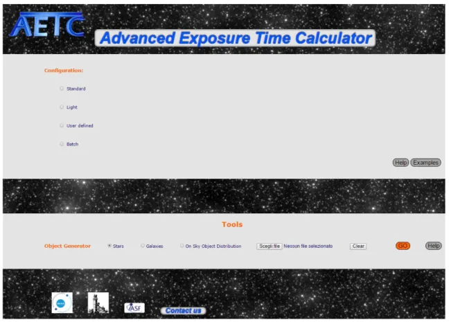
Figure 1. AETC (version 4.0) main web interface.

Proc. of SPIE Vol. 9911 99112U-2

(5)

From the main page (Figure 1) it is possible to load the configuration selecting among various options:

• Standard: pre-defined list of instruments (Table 1) with the possibility to modify all inputs; it is also possible to configure a completely new instrument from scratch;

Telescope Instrument HST WFPC2 JWST NIRcam VLT FORS ELT MICADO TNG NICS DOLORES REM ROSS REMIR LBT LBC

Table 1. List of the pre-defined instrument configurations available.

• Light: list of existing instruments with fixed telescope, site and detector characteristics; it is possible to select only observation parameters;

• User defined: configuration totally provided by the user;

• Batch: a user provided list of instrument configuration files to execute in batch mode in order to run multiple simulations automatically.

Once the selected configuration is loaded, the interface to enter all input parameters becomes available. Default values are already set in input fields. Each input can be a value, an array or a list.

The list of the parameters is summarized in Table 2:

Telescope and Instrument Specification

Primary mirror Value

Number of reflections Value

Fraction of obstruction Value

Platescale Value

Readout noise Value

Mirror Reflectivity Array

Instrument Efficiency Array

Detector Efficiency Array

Sky

Air mass Value

Sky Brightness Array

Atmospheric Absorption Array

Observation Parameters

Observation band Array

Exposure time Value

Number of exposures Value

(6)

Ariz

Home Configuration Telescope and Instrument Specification Sky Observation Parameters Source Specifications Image Simulator Results Configuration file Batch mode Advanced Help object generator Stars Galaxies Sky Field Extractor On sky abject distribution

INAF

(43F,

Introduction

The Advanced Exposure Orne Calcuator lAEfC) N a tool to simulate mages of astroplysbal objects obtained wan any commnar n or telescope, instrument and givenpassion using a suable set or parameters That define the configuration arse equipment used for Ne observalbns. The tool provides count rates and as dstriburbn over the focal pane, through the proper dennnbn arse PSF, or Mealy any telescope equipped wan an imager provided Nat as configuration H assessed. Moreover genaltd simulation ortie observed fields can be simulated including stars, galaxies and more complex aber. proNding template orme targets

Fabmo, R., Fantinel, O., Ilsengnl, M 2011 Prec. SPIE 8135. 813523 120111 IPDF1

Some example or Images produced by AETC:

e

.II

Nuclear star cluster_ MICADO @E -ELT Nearby galaxy cluster. W FC @INT M51 -llke galgos @Z=2.4 MICADO @E -ELT

Aperture Value PSF model Array Source Specification Redshift Value SED Array Flux Array Image Simulator X-size Value Y-size Value Gain Value FPN Value Dark Value

Rad min Value

Saturation level Value

Threshold Value

System Coordinates Value

Spline Degree Value

Number of used PSF Value

Convolution Value Table 2. List of the configurable parameters.

On the same interface it is also possible to select the results to be displayed in the output page, checking the available boxes.

2.2 Help & examples

An exhaustive help is reachable from the main interface; for each field the input meaning, the range of possible values and examples are illustrated.

Figure 2. AETC help main page.

(7)

Configuration:

O Standard O Light O User defined

® Batch Browse... No file seleded. Clear e -mail address (LOAD)

Aperture Output Signals:

S/N area: 12.6 px

Collecting area: 11009347.0298 cm2

Zero Point: 30.12

Source: 3.598228e +06 ph /aper /expT StoN: 1862.75

Background: 1.328349e +05 ph /aper /expT (10.57 ph /sec /px)

Effective wavelenght: 16475.0A

Extinction at Aeff: 0.0

Example page shows three complete simulations obtained with AETC: a star field with LBC@LBT, a star cluster with MICADO@E-ELT and a cluster of galaxies with a custom instrument. All steps needed to reproduce these simulations are explained in detail.

2.3 Modes

The tool can run in interactive and in batch modes. In interactive mode the user fills the requested fields in the form, selects the output options and then AETC shows the results. In batch mode (see Figure 3) a large number of simulations can be executed automatically. Inputs are passed to the tool in a single gzipped file containing all configuration files. At the end of simulations a link to the result is provided.

Figure 3. When “Batch” mode is selected in the AETC main page, the user is asked to provide a gzipped file containing the configuration files and an email address to receive the link to the result.

3. SIMULATION PIPELINE

The simulation pipeline takes a user selectable set of input parameters and creates the output, including the simulated image. The process can be broken down into the configuration builder and the image builder.

3.1 Configuration builder

The configuration builder has been developed in PYTHON and makes use of NUMPY, SCIPY and MATHLAB packages. The computed results include number of counts for a selected object and background in the aperture and the Signal to Noise Ratio.

Figure 4. Output counts and the expected Signal-to-Noise ratio produced by the configuration builder.

(8)

Sensitivity Graphs

Input source:

MicaooH (14800.0 - 18200.0) Stars vega ExpT 1000

1.61e -18 1.4 á 1.2 E á 1.0 0.8 4500000 4000000 3500000 3000000 rv 2500000 2000000 1500000 1000000 500000 throughput:

MicadoH (14800.0 - 18200.0) Stars vega ExpT 1000

44500 15000 15500 16000 16500 17000 17500 18000 18500 12500 15000 15500 16000 16500 17000 17500 18000 18500 50 40 30 c 0 0 20 10 Wavelength (A) s<y 1).J; ,(1..2.1.11'0:

(+acaal ,l-l'cUU.O 1.82U::.01 v l 10,.0

1600 1400 1200 1000 c 800 600 400 200 Wavelength (Al output source:

MicadoH (14800.0 - 18200.0) Stars vega ExpT 1000

12500 15000 15500 16000 16500 17000 17500 18000 18500 14500 15000 15500 16000 16500 17000 17500 18000 18500

Wavelength (A) Wavelenght (A)

Signal /Noise (Point Source)

S/N 1862.7 Aperture Diameter 0.012aresec ExpT 1000sec Mag 20 System Vega

105 z ",71 104 103 102 101 10° 102 103 104

Exp time (sec)

Values of input source, throughput, sky background and output source are then extended in the range of the Observation band and displayed (Figure 5).

Figure 5. Plots of the selected input source, passband and the throughput.

Figure 6. Plot the trend of the S/N against the exposure time for a wide range of integration times

(9)

l Stars

EGalaxies

El Objects

2Functions

Browse... No file selected. IClear E Upload Browse... No file selected. I dear 0 Upload

Browse... No file selected.

Clear © Upload Object Template Files

Clear EUpload Function Template Files

Browse... No file selected. Upload

Browse... I No file selected. 0 Upload The S/N is computed for a point like source; input flux is combined with the telescope efficiency parameters and the background level and finally integrated on the aperture diameter defined by the user. The S/N is then extended in a range of different exposure times. The S/N curves at different limiting magnitudes are also computed (Figure 6)

Moreover, the configuration builder provides all parameters to Image Builder through an ascii file.

3.2 Image Builder

The module for generating the simulated images has been developed in IDL. The tool takes in input the adopted configuration of the instrument, in the format produced by the configuration builder, the PSF and a set of files containing the positions and the properties of the sources to be included in the image.

Sources can be of different types: stars, galaxies, templates and functions (at the moment, only 2d Gaussian function has been implemented but more kind of functions will be available in the future) to model complex targets. For each kind of sources to be included in the simulation, an asci file containing the list of the appropriate source parameters must be uploaded (see Figure 7). The format of the files is explained in the help page of the image simulator.

Figure 7. Section of the web interface to upload the list of the objects to be included in the simulated image. The star file must contain a list of the [x,y] coordinates and magnitude of each star.

Galaxies are modeled with a Sersic law I(r) (eq.1): the user must provide for each galaxy the coordinates of the center, the total magnitude, the index of the Sersic law, the half-light radius, the ellipticity and the position angle.

( )

(

₍

)

₎

( )

( ) ⎟⎟⎟_⎠ ⎞ ⎜⎜ ⎜ ⎝ ⎛ − ⋅ − − − − − ⋅ ⋅ Γ − = 1 331 . 0 2 2 2 331 . 0 2 0 1 1 2 2 331 . 0 2 n rn e n n e r n n n e I r I ε π (1) where r is given by the relationship:

(

)

(

)

(

)

2

(

0

)

0 2 0 0 1 cos ) ( sin sin cos 1 ) , ( ⎟ ⎠ ⎞ ⎜ ⎝ ⎛ − − + − − + − + − = ε θ θ θ θ y y x x y y x x r y x r e (2)

Complex objects can be simulated from a user-provided template: this allows introducing sources with complex features, just providing an image of suitable resolution. The template must be a fits image with the background subtracted. The “object” file is a text file listing:

• x,y coordinates of the object

• magnitude of the object in the adopted photometric system • template to be used

• size (in arcsec) in the simulated output frame

(10)

“Functions” is a generalized kind of sources, which includes also stars and galaxies, but add the possibility of using simple functions to describe any kind of objects by a combination of them.

The sources models are convolved with the PSF. One of the key features is how the simulator can manage the PSF: it can support a large range of types, from very simple models, constant in the field of view, to complex models taking in account the spatial dependency.

The PSF can be seeing limited, modeled by a Gaussian or Moffat function of given FWHM, or the user can provide a model in form of a 1D radial average brightness profile or 2D fits image.

For modeling variable PSF there are a two options available:

1) provide a 3-D fits data cube containing 2D PSF images computed (or measured) at different positions in the field of view (the position of the PSF in the data cube are listed in a separate text file). The PSF is then computed at each position of interest (x0,y0) by a weighted average of the n (n is an user-defined parameter) closest PSF included in the data cube, weighting each PSF template with the inverse of the distance from x0,y0

2) provide a stretching map that describes the changes (not necessarily on a grid) of the PSF model in terms of ellipticity, FWHM and position angle along the FoV, compared to a reference fits image describing the PSF at a given point. The first option is particularly suitable for instruments in development (the PSF data cube can be built using a ray tracing software), whereas the second one is thought for existing instruments, since the variation of the ellipticity, FWHM and position angle can be derived by analysis of reference stars in previously acquired images.

The last steps of the simulation are 1) adding the noise (optional), which is modeled taking in account: • Shot noise

• Readout noise

• Dark current of the detector • Fixed pattern noise

and 2) convert photons in ADU considering the gain and the saturation level of the detector.

To save computation time, all the simulated sources can be computed up to a radius where their contribution goes below a given fraction of the background noise. The fraction of flux external to the computed radius is then considered as a diffuse component and added to the background. Sources outside the simulated area, but close enough that their wings can give a contribution, are also considered, in order to avoid edge effects in the diffuse count rate.

In general, since the previous versions [1], in version 4.0 efforts have been devoted to limit memory occupancy and computation time.

3.3 Object generator

The Object Generator (OG) is an utility tool for creating lists of astronomical objects, to help the user in building the input files of the sources to be included in the AETC simulated images.

The tool is divided in two parts: in the first part, the ''on sky'' section, it is possible to create lists of stars or galaxies according to a selected flux and spatial distribution on the sky (Figure 8). In the second part of the tool the object distribution is converted into a list of targets on the chosen detector, based on the platescale of the selected instrument.

(11)

On Sky Object Distribution Stellar population: Total objects: 1501 Brightest Meg: 18.0 Faintest Mag: 24.0

Field of liiew: 600.0 Miser) Magnitude Distribution: Power law Index: 0.3 Spatial Distribution: User deemed law bumble: Spatialdst0b.txt

Magnitude Histogram

MO

On Sky Object Distribution (aresec): star2015 02 10 10 111 M.bR

On StellarPapalailaa. Total objecta:10p Brightest Kng: 151 rainten y20.0

S Object Distribution

Magnitude Distribution: Spatial Distribution: Lin

Userdefinaed lawfromel: Gal MOgDistnb.Dd ar

Sway: effective ramos..020.01inea =1.0 seismo super,: 1.0.4.0 kaea=1.0 Elliptic] ty: 0.0-0.7 lmea=1.0 PA, 0.0-100.0kae. =(.0 Magnitudilintogram Sky

xso

On Sky Object Distribution ( aresec). galaay2O15 02 18 10 52 14.5(1 11

Figure 8. Example of Object Generator outputs: (left) a list of 1500 stars distributed according to a radial distribution profile; (right) a list of 100 galaxies uniformly distributed in the FoV.

4. EXAMPLES

As previously mentioned, AETC has been developed during the Phase A study of MICADO. MICADO (Multi-AO Imaging Camera for Deep Observations) is an IR camera designed for EELT to provide diffraction-limited imaging over a ~1 arcmin FoV. To explore the new challenges that we could face using this unique instrument, we started to study the feasibility of a number of science cases. For each of them, we simulated imaging observations with AETC and performed a detailed photometric analysis on the images. The results were used to evaluate the photometric performances of the instrument and then asses the reliability of the scientific results.

Some examples are summarized in the following paragraphs to briefly illustrate AETC capabilities, for more details see references [2-7].

4.1 Nuclear Star Clusters (NSC)

The nuclei of galaxies are extraordinary laboratories to probe the processes that lead to the formation of nowadays galaxies. The properties of the nuclear regions are in fact thought to be linked with the formation history of the galaxies where the collapse of gas and merging events may play a relevant role for different types of galaxies and environments. Various phenomena characterize these nuclei such as super-massive black holes (SMBHs), active galactic nuclei, central starbursts, and extreme stellar densities. All these phenomena are likely connected to the global properties of their host galaxies, and co-evolution of the various components is invoked to account for the observed correlations.

In order to age-date the resolved stellar population of the NSC we need to disentangle the cluster members from the stars of its host galaxy. In the central parts of the cluster, the stellar field is dominated by the cluster members, but the stellar density is very high and stars are blended, decreasing the accuracy of the photometry. On the other hand, in the external regions, where photometry is more accurate, the host galaxy body population contribution becomes important, and it is more difficult to disentangle the two components. The interplay of these two factors determines the intermediate region where photometry can be accurate enough and the host contribution is low enough to allow us to measure reliable age and metallicity for the cluster stellar populations. Thus, the possibility of characterizing the stellar population of NSCs depends on a few parameters, e.g. the distance of the host galaxy and the core radius of the cluster which control the crowding conditions. In addition, for a given distance, the older the NSC the fainter are the stars at the turn off, which makes it more difficult to determine its age. In order to exploit the capabilities of ELTs to investigate NSCs, we have simulated a number of cases with different age and at different distance, simulating observations with both MICADO@E-ELT (in I, J, H, K band) and IRIS (InfraRed Imaging Spectrograph) at TMT (the Thirty Meter Telescope, that will be built at Mauna Kea, Hawaii) in Z and J band.

All simulated images used in the work [5] were produced using AETC with a total integration time of 3h. For IRIS, AETC has been configured with the specifications listed in ref. [9] and the PSF has been kindly provided by S. Wright.

(12)

y

:

--1

.

' .

`

.

'

^

,

.-.,

'

, # or.

¡',

.

..-y

A

r.

.=;

. .

4

` ' 4 .

,. i

.': *_lr

'r.

.

-`

.

* -

.

.1

For MICADO, we used the specifications given in ref. [8] and the June 2012 release of the MAORY (Multi-conjugate Adaptive Optics post focal RelaY) available at the official site:

http://www.bo.astro.it/maory/Maory/Welcome.html

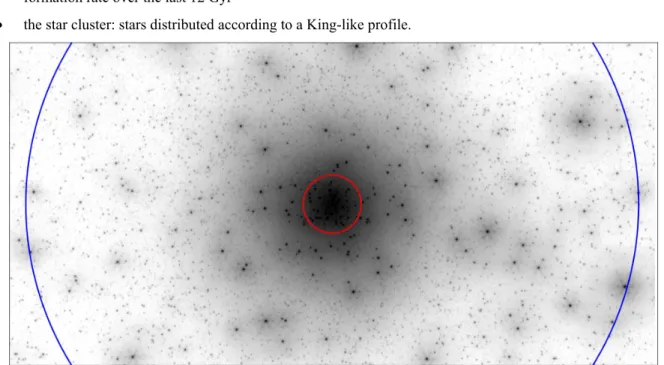
An example of a section of a simulated image with 3h exposure time is shown in Figure 9. The input star list included two components for a total of 465567 stars:

• the host galaxy body: spatially uniform distribution of stars, magnitudes calculated assuming a constant star formation rate over the last 12 Gyr

• the star cluster: stars distributed according to a King-like profile.

Figure 9. Zoom of a 6’’×3’’ region of a J-band simulated with MICADO@E-ELT. The circles shows effective radius (0’’.27, in red) and tidal radius (2’’.85, in blue) of the cluster.

Figure 10 shows a comparison of the same region simulated with different instruments.

4.2 High-z galaxies

To evaluate the accuracy with which will be possible to characterize the properties of high redshift galaxies with MICADO observations [7], we performed simulated observations of high-z galaxies using template images obtained

Figure 10. 1’’×1’’ E-ELT (left), TMT (center), and JWST (right) images at 6 re from the

centre of the 1 Gyr old NSC at 2 Mpc. In the left panel the red circles shows J=28 mag stars, corresponding to the main-sequence turn-off magnitude.

(13)

HST/WFC3 F475W ARP 142

4100*--00.

Micado H z=3 NirCAM H z=3 Hi"

gip

HST /ACS F435W NGC 6217 Micado J z=2 NirCAM J z=2

from high-resolution observations of nearby galaxies. To this aim, we looked for Advanced Camera for Survey (ACS) and/or WFC3 observations of galaxies with different morphologies in the HST archive.

We selected observations in photometric bands that roughly correspond to J and H (H and K) when redshifted at z∼2 (∼ 3). Figure 11 shows an example of simulations obtained with two different templates:

• image in the filters F435W of NGC 6217 (z = 0.004), a star-forming barred spiral galaxy;

• images in filters F475W of ARP 142 (z = 0.023), a violent merger of an elliptical galaxy with a disrupting gas-rich galaxy.

We removed from the original HST images all foreground stars, background galaxies, cosmic rays and artefacts. We then used AETC to produce MICADO and JWST simulated observations with a total integration time of 3 hours. The total flux and angular size of the templates were rescaled to match the magnitude and size of galaxies at redshift 2 and 3.

5. CONCLUSIONS

We realized and provided to the scientific community a flexible exposure time computation tool, with image simulation capability, which can be used for a wide range of existing instrumentation or for predicting the performance of new instrumentation. It can be useful to study feasibility of science programs both with existing and future facilities, and to tune the design parameters of new instruments driven by the main science cases.

Figure 11. Simulations of MICADO (central panels) and NIRCam (right panels) H-band observations of galaxies at z ∼ 2 (top panels) and z ∼ 3 (bottom panels) obtained using as templates HST observations of nearby galaxies (left panels) in photometric bands roughly corresponding to the H band when redshifted at z ∼ 2 or 3. Images are simulated with exposure time = 3h.

(14)

REFERENCES

[1] Falomo, R., Fantinel, D., Uslenghi, M., “AETC: Advanced Exposure Time Calculator”, SPIE 8135 (2011) [2] Greggio, L., Falomo, R., Uslenghi, M., “Studying stellar halos with future facilities”, Proc. IAU Symposium

317 "The General Assembly of Stellar Halos: Structure, Origin and Evolution, arXiv:1510.03181

[3] Greggio, L., Gullieuszik, M., Falomo, R., Fantinel, D., Uslenghi, M., “Properties of High Redshift Galaxies in the ELTs Era”, IAU General Assembly, Meeting #29 (2015)

[4] Schreiber, L., Greggio, L., Falomo, R., Fantinel, D., Uslenghi, M., “Studying the metallicity gradient in Virgo ellipticals with European-Extremely Large Telescope photometry of resolved stars”, MNRAS 437, issue 3, p.2966 (2014)

[5] Gullieuszik, M., Greggio, L., Falomo, R., Schreiber, L., Uslenghi, M., “Probing the nuclear star cluster of galaxies with extremely large telescopes”, A&A 568 (2014)

[6] Greggio, L., Falomo, R., Zaggia, S., Fantinel, D., Uslenghi, M., “Resolved Stellar Population of Distant Galaxies in the ELT Era”, PASP 124, issue 917, p.653 (2012)

[7] Gullieuszik, M., Falomo, R., Greggio, L., Uslenghi, M., Fantinel, D., “Exploring high-z galaxies with the E-ELT”, A&A, in press

[8] Davies, R., Ageorges, N., Barl, L., et al., in Ground-based and Airborne Instrumentation for Astronomy III, eds. I. S. McLean, S. K. Ramsay, & H. Takami, Proc. SPIE, 7735, 77352A (2010)

[9] Wright, S. A., Barton, E. J., Larkin, J. E., et al., in Ground-based and Airborne Instrumentation for Astronomy III, eds. I. S. McLean, S. K. Ramsay, & H. Takami, Proc. SPIE, 7735, 77357P (2010)