University of Pisa
Sant’Anna School of Advanced Studies
Master of Science in Economics Department of Economics and Management
Financial contagion in inter-bank
networks: a computational model
with real shocks
A.Y. 2013/2014
Supervisors:
Prof. Giulio Bottazzi Dr. Fabio Vanni
Candidate Alessandro De Sanctis
Contents
List of figures iii
1 Introduction 9
2 Literature review 13
2.1 Network application to financial systems . . . 14
2.2 The model of Gai and Kapadia (2010) . . . 16
3 The model 22 3.1 The logic of the model . . . 23
3.1.1 Assumptions . . . 24
3.1.2 The algorithm: 1) initializing the model . . . 27
3.1.3 The algorithm: 2) shock trasmission . . . 28
4 Simulations results 30 4.1 The benchmark case . . . 33
4.1.1 Extent and frequency of contagion . . . 34
4.1.2 Dynamic of the model . . . 36
4.2 Varying η . . . 48
4.2.1 Extent and frequency of contagion . . . 48
4.2.2 Dynamic of the model . . . 50
4.3 Varying θ . . . 55
4.3.1 Extent and frequency of contagion . . . 55
4.4 Varying pF . . . 62
4.4.1 Extent and frequency of contagion . . . 62
4.4.2 Dynamic of the model . . . 64
4.5 Varying δ . . . 68
4.5.1 Extent and frequency of contagion . . . 68
4.5.2 Dynamic of the model . . . 69
5 Conclusions 73
Appendices 75
A - Network theory 75
List of Figures
2.1 Gai Kapadia benchmark model . . . 21
3.1 Balance sheet structure . . . 25
4.1 Benchmark case: extent and frequency of contagion . . . 34
4.2 Benchmark case: average number of rounds . . . 36
4.3 Benchmark case: average number of rounds and standard devistions . 37 4.4 Benchmark case: total number of defaults . . . 38
4.5 Benchmark case: defaults for rounds from 1 to 6 . . . 39
4.6 Benchmark case: defaults for rounds from 7 to 12 . . . 40
4.7 Benchmark case: defaults for rounds from 1 to 6 given contagion . . . 41
4.8 Benchmark case: defaults for rounds from 7 to 12 given contagion . . 42
4.9 Benchmark case: aggregate loss per round . . . 43
4.10 Benchmark case: loss per round from 1 to 6 . . . 44
4.11 Benchmark case: loss per round from 7 to 12 . . . 45
4.12 Benchmark case: loss per round from 1 to 6 conditional on contagion 46 4.13 Benchmark case: loss per round from 7 to 12 conditional on contagion 47 4.14 Varying η: extent and frequency of contagion . . . 49
4.15 Varying η: average number of rounds . . . 50
4.16 Varying η: average number of rounds with standard deviations . . . . 51
4.17 Varying η: total number of defaults . . . 52
4.18 Varying η: aggregate loss per round . . . 54
4.19 Varying θ: extent and frequency of contagion . . . 56
4.21 Varying θ: average number of rounds with standard deviations . . . . 58
4.22 Varying θ: total number of defaults . . . 59
4.23 Varying θ: aggregate loss per round . . . 61
4.24 Varying pF: extent and frequency of contagion . . . 63
4.25 Varying pF: average number of rounds . . . 64
4.26 Varying pF: average number of rounds with standard deviations . . . 65
4.27 Varying pF: total number of defaults . . . 66
4.28 Varying pF: aggregate loss per round . . . 67
4.29 Varying δ: extent and frequency of contagion . . . 68
4.30 Varying δ: average number of rounds . . . 69
4.31 Varying δ: average number of rounds with standard deviations . . . . 70
4.32 Varying δ: total number of defaults . . . 71
4.33 Varying δ: aggregate loss per round . . . 72
5.1 An example of network . . . 76
Chapter 1
Introduction
Over the last forty years world’s economy has experienced an unparallel process of globalization both in terms of goods traded, both in terms of capital movement and financial exchanges. For what concerns the financial sector, intended in a broad sense as the ensemble of banks, insurances, funds and so on, the willingness to attempt an even higher level of risk diversification , the advances in terms of finan-cial engeneering (for example securitization) and the diffusion on large scale of new types of contracts (such as derivatives, credit default swaps and collateralised debt obligations) , have caused an increase in the level of complexity and connectivity of the finalncial system, with the result that today’s financial insitutions are directly or indirectly connected with many more counterparts (within the financial system itself and with the real side of the economy) all over the world than few decades ago.
This reduction of the “world’s size” from an XXL to a SMALL (Friedman, 2006) has brought, togheter with numerous advantages, also some potential drawbacks, which, as far as concern the financial system, have become clearer with the financial crises started in late 2007 in the United States.
In that case, the initial local shock represented by the inability to pay their home mortgages by hundreds of american households, has ended up into a global financial crises, then turned into an economics crises at world scale. The most famous and striking event of this crises, even at the level of collective imaginary, has been the
failure of Lehman Brothers in 2008.
That default has not been isolated, but it has been followed by a series of deafults and bailouts all over the world, from United States (AIG, Fannie Mae, Freddie Mac, Bearn Sterns, Merrill Lynch, Countrywide Financial just to name a few) to Unitied Kingdom (for instance Northen Rock), from Ireland (Anglo Irish Bank) to Spain (Bankia and Caja de Ahorros Castilla La Mancha between the others), from Iceland (for example Landsbanki, Glitnir, Kaupthing Bank) to Netherlands (ABN AMRO). This sequence of bailouts has shown how the intricate network of claims and obli-gations links the financial institutions all over the world, so that the functioning of one institution can affect the survival of another, appearently far and not influenced, institution (in many respects resembling the so called butterfly effect ), or even be crucial for the whole system (too big to fail argument). The high degree of connc-tivity among banks, hedge funds, insurance companies and in general of financial intermediaries which has been reached by the modern financial system, turned out to be a key determinant for the outbreak of a systemic crises, that is of a crises affecting the whole system.
As pointed out by Reinhart and Rogoff (2009) in their study of financial crises, what happened in 2008 was not an exception; paraphrasing the title of their book, “that time was not different”. Indeed, by looking at the data that they have collected, banking crises have revealed to be a periodic event of economies: from 1800 to 2010 United States have experienced 31 banking crises1, United Kingdom 25, France and
Germany 16, Italy 18, Japan 17 (Reinhart, 2010), (Reinhart & Rogoff, 2010). Given the relative high frequency of banking crises and the enormous costs related to them for taxpayers, governments (public debt) and the economy as a whole (for instance loss of potential output), a better understanding of how crises occur and which can be their cosequences seems required, both to better forecast them, both to develope policy prescriptions in order to prevent them.
1In (Reinhart, 2010) the two authors define a banking crises as an event in which there are “bank
runs that lead to the closure, merging, or takover by the public sector of one or more financial institutions and if there are no runs, the closure, merging, take-over or large-scale government assistance of an important financial institution (or group of institutions) that marks the start of a string of similar outcomes for other financial instituitions”
As pointed out in the previous paragraphs, the structure of modern financial sys-tem is characterized by an ensable of different agents highly interconnected between them by their reciprocal claims and obligations, which give rise to an intricate web of debit/credit relations that link the balance sheets of a wide variety of intermedi-aries (Gai & Kapadia, 2010). A natural way to think at this system is to see it as a complex network, that is as “a collection of points joined together in pairs by lines. [...] points are referred to as vertices or nodes and the lines are referred to as edges” ((Newman, 2010) p. 1).
The developements in the theory of networks of the last twenty years and its re-cent application to economics and finance have revelaed how much this approach is well suitable in modelling financial system and have gave rise to a growing body of literature on financial networks. The present work engages in this filed of research by developing a simple model of financial network and performing a computational study to assess if and to what extent a real shock, such as the bankruptcy of a firm (due for example to a slump in the aggregate demand), can be transmitted to the financial system and determine a systemic crisis.
The work draws from the growing body of literature regarding the contagion in fi-nancial network, which has flourished in the recent years, however, differently from the majority of the studies of this kind, the present comprises a formalization of the real side of the economy represented by firms2 and of the interaction between banks
and firms.
One of the main benchmarks of the work is the model provided by Gai and Kapa-dia (2010): following these two authors the financial network is constructed on the basis of mutual claims and obligations between financial instituions. However, the model presented here extends the one of Gai and Kapadia extends the one of Gai
2In what follows it is assumed for simplicity that the real side of the economy is constituted only
by firms, however for they way in which firms are modelled in this work it would also be possible to think at them as households or as households and firms without altering the analysis or making any conceptual mistake. However, we decided to consider and to call them firms because there are more data available on the defaults of firms rather than on houselhods, which are useful to parametrising the model; even more important is that, nothwithstanding the fact the the subprime crisis has been triggered by the “defaults” of hoseholds, firms are bigger than hoseholds in terms of assets and loans received and therefore are likely to be more relevant in determining a crisis.
and Kapadia by adding a second layer in the network structure which represents the real side of the economy through firms: in this new set up, exogenous shocks are no longer represented by a “big” single failure of a bank, but by a multiplicity of “small” shocks hitting different banks, represented by the default of a given number of firms; therefore a priori we do not have the guarantee that the banking system will be affected (for example by triggering a cascade of banks defaults) by a real shock.
The model developed departs from the baseline model of Gai and Kapadia (2010) also in some others respects, such as heterogeneity of banks’ assets and number of inter-bank links, as it will be discussed more in detail in the next chapters. The work studies, under different settings and values of the paramenters, how shocks propagate through the financial network, which is the resilience of such a system and to what extent the final outcome depends on finer details like the assumptions about balance sheet composition.
Although the model that will be presented in the next chapters is a very stylized representation of reality and the interplay between the financial and the real part may appear oversimplified, it is able to provide some policy suggestions in order to analyse the financial stability, to increase the resilience of the system and to reduce the probability and the spread of systemic crises. Moreover, notwithstanding its limits, it represents a first attempt to link two worlds which have been too often treated separately, constituting a useful starting point for further research.
Chapter 2
Literature review
In this chapter we will make a short review of the literature on contagion in financial networks, doing a brief history of the main theoretical and empirical achievements. We will also give an overview of the most relevant models developed and of their features and findings, devoting greater attention to the ones which have represented a particular important reference point for this work.
Even if the network applications to financial systems constitute a relatively recent field of research, the issues related with this strand of literature are already many and diverse, therefore to provide a complete tretment of all of them would be im-possibile and it is not the aim of the work3.
For our purposes it is just worth noting that the model presented here leaves out several issues regarding network modellization of financial systems, such as the en-dogenous network formation, the optimal network structure and the choice of the network model. Those issues, however important, have been left apart from the dis-cussion for three main reasons: first, to keep things as simple as possible, avoiding excessive complication of the model, which would have resulted in too long compu-tational times; second, to preserve some form of comparability with the benchmark models; third, because there is no unanimous consensus between scholars on what
best reflects empirical reality4 5.
Before proceeding to the next section, the reader which is not familiar with the network terminology that will be used from now on, can refer to Appendix A on network theory for clarifications.
2.1
Network application to financial systems
Over the last fifteen years, with a faster pace after the cirses of 2008, network models began to be extensively applied to study the resilience of banking systems (Allen & Babus, 2009; Hasman, 2013).
The pioneering work in the field is the one of Allen and Gale (Allen & Gale, 2000) who were the first to show how a complete network structure is able to absorb id-iosyncratic shocks hitting a single bank, while incomplete networks might allow the spread throughout the system.
In their work financial contagion is modeled as an equilibrium phenomenon and it is caused by liquidity preference shocks. In their framework the possibility of con-tagion depends strongly on the completeness of the structure of network: complete network structures are more robust than incomplete structures
After their work, many other research has been carried out, mainly thoretical, but also empirical, nothwitstanding the difficulties in obtaining data.
For example (Nier et al. , 2007) study a interbank random network of 25 banks to analyses how systemic risk depends on the structure of the banking system and show that, all else equal, contagion is a non-monotonic function of the number of interbank connections.
More complex model and different network structures, which aim at mimic more closely some emipirically observed fetures of financial systems have then been used,
4For example there is no clear evidence on which structure exhibits real world banking networks:
although some real-world banking networks may have core-periphery structures and tiering, such as the Austrian (Boss et al. , 2004) and German (Craig & Von Peter, 2014) interbank markets, the empirical data are limited.
5For a discussion of these topics see (Leitner, 2005; Gale & Kariv, 2007; Castiglionesi & Navarro,
for example the one developed by (Montagna & Lux, 2013). In this model there are two interesting aspects: first, the analysis on the dynamics of contagion that the two authors perform, which studies in detail what happens in each default cascades, how many banks fail and which is the aggregate loss. A second interesting aspect is that they assume a scale-free network with preferential attachment, where the probability of having a link is dependet on the number of links already active for a node. In other words networks are produced according to a fitness algorithm, able to reproduce the disassortative behavior, the power laws in the degree distributions and the power laws in the distribution of bank sizes which have been frequanlty documented by empirical studies.
Another relevant model, which is the one more close to the approch that we will use later on, is the one recently published by (Anand et al. , 2013), in which for the first time, a real shock is introduced in this type of models.
Indeed this paper tries to link the real and the financial side of the economy exam-ining the role of macroeconomic fluctuations, assets market liquidity and network structure in determining contagion and aggregate loss. The results show the impor-tance of fire-sales externalities and feedback effects due to the reduction of credit on the economy and the mortality rate of the firms.
To summarize, the literature on financial contagion has enucleated a series of find-ings and interesting aspects. First of all two different type of causes of contagion have been pointed out: in contagion occurred through indirect balance-sheet linkages and contagion due to direct linkages. Second, an ambiguous role of diversification has been observed. Third, the degree of connectivity of the system has been deteced as a key determinant of contagion. Finally different initial shocks can be possible and they have different effects on the systems.
We will now describe more in details the model developed in (Gai & Kapadia, 2010), since it will represent our main benchmark point trough all the chapters.
2.2
The model of Gai and Kapadia (2010)
The present section summarizes the main features of the model of Gai and Kapadia (2010), therefore it necessarily draws a lot from the original paper, in particular from section 2 and subsection 3.1.
The paper is one of the most cited in current literature and represents one of the major contributions to this field, as well as our main starting point in the builiding our model.
The two authors develop a model6 of contagion in financial networks which studies
how an initial exogenous shock, represented by the bankrupt of a bank, is trans-mitted thorugh the network and which is the likelihood and extent of contagion for different degrees of connectivity, recovery rates and levels of liquidity risk.
The model manage to capture two key sources of contagion: the so called direct con-tagion, which goes through the interbank channels, and the indirect concon-tagion, that affects the non-interbank assets inscribed in banks’ balance sheet (such as mortgages, bonds, shares). The first source of contagion reflects the direct influence which the default of a bank can have on linked banks, while the second source reflects the indirect influence of a fall in the price (and so in the value)7 of assets owned by banks led by the failure of others, not necessarily linked, banks.
The authors consider a financial network with arbitrary structure in which N finan-cial intermediaries8 - banks for simplicity - are randomly connected one with the
other through their reciprocal claims.
In the view of graph theory banks represent the nodes of the network and the credit/debit relationships represent the links (or edges) between banks. Links are weighted for the value of the claim/duty reported in the balance sheet of the bank. In particular, if a bank i has a credit toward a bank j, this credit is represented by
6The model is solved both analytically, by means of probability generating function techniques,
both numerically through computer simulations. As we are primarily interested in the computa-tional part of their work, in what follows we will not discuss the analytical solution provided by the authors.
7Such situation is more likely to occur when the market for financial assets is illiquid (cfr.
Gai-Kapadia 2010, p.3)
8With financial intermediaries we mean banks, insurance companies, hedge funds, pension funds
an incoming link for bank i and an outgoing link for bank j. The resulting network structure is therefore directed and weighted9.
Practically the model is impelmented thorugh the following steps.
Building the Financial Network First the financial network is constructed passing over all possible directed (non-weighted) links and activating each one with indepedent proabbility. In other words, one by one all nodes are considered and an incoming link is created with a proability p. The result is a (Poisson) random graph Γ (N, p)10that is mathematically represented by an N × N matrix, called adjacency matrix, which main diagonal is made of null elements (since links starting and ending in the same nodes are not allowed, that is a bank can not have a credit/debt with itself). In their simulation Gai and Kapadia consider a (Poisson) random graph composed of 1,000 nodes.
Initializing the Model At time t = 0 the model is initialized filling up the banks’ balance sheets in accordance with the following assumptions:
a) the same amount of interbank assets is assigned to every bank, i.e. Aib
i,0 = Aibj,0
∀i, j. In addition, interbank assets are assumed to be evenly distributed among all active links, therefore the credit owed from bank j to bank i is equal to the amount of interbank assets of bank i divided by the number of incoming link of bank i ;
b) from the previous assumption derives that interbank liabilities are endoge-nously determinated since each interbank assets Aib
i,j corresponds to an
inter-bank liability Lib
j,i for another bank;
c) total assets are assumed to be constituted for the 20% of interbank asstes and for the 80% of non-interbank assets11, therefore we can write:
Atoti,t = Aibi,t+ Ami,t
9See Appendix A for a definition of directed and weighted network 10See Appendix A for a definition of (Poisson) random graph.
Aibi,0 = 0.2 · Atoti,0 Ami,0 = 0.8 · Atoti,0
Ami,0 = 4 · Aibi,0 (2.1)
d) the capital buffer Ki,0 of a generic bank is set to be the 4% of its total assets,
therefore manipulating the previously established relations we can write
Ki,0 =
Aibi,0
5 (2.2)
It worth noting that, given these assumptions, at time t = 0 all banks are perfectly homogeneous with respect to their total assets and capital buffer and that it is possible to express all these variables in terms of interbank assets;
e) finally the liability side of the balace sheet is topped-up with deposits in order to respect the accounting identities, that is:
Di,0 = Atoti,0 − L ib
i,0− Ki,0 (2.3)
Note that Di,0 will not change during the dynamics of the model, i.e. it is
equal to its initial value ∀t.
The mechanism of contagion The dynamics of the model proceeds quite me-chanically in the following way. All banks are initially solvent, then at time t = 1 the network is perturbed by the default 12 of a single bank selected randomly. In
practice the default is generated by wiping out all the external asstes of the bank, that is setting Am
i = 0. This is sufficient to ensure that the bank will fail because:
Aibi,0+ 0 − Libi,0− Di,0 ≤ 0
Aibi,0− Libi,0− (24 5 A ib i,0− L ib i,0) ≤ 0 −19 5 A ib i,0 ≤ 0
which is true ∀Aib i,0 ≥ 0.
This initial shock can be absorbed or amplified and in principle can trigger a cascade of defaults. A zero recovery assumption is made, that is the failed bank is assumed to default of all its interbank liabilites, thus causing a complete loss to creditor banks which mark down to zero the value of their claim13. If losses exceed the capital buffer of the bank, then it is set into default too and another round of markdowns begins, otherwise capital is simply reduced in order to absorb the loss. This iterative process keeps going until no further bank defaults.
From the balance sheet defined above, it is possible to derive the condition for
12This intial default can be see as an idiosyncratic shock or as the result of an aggregate shock
that has had particularly negative effects on a single bank.
13In some of the numerical simulations performed by the authors show that their results are
ro-bust to relaxing this assumption. However, as we will see later in this work, the weaker assumption that is made is quite questionable.
solvency of a generic bank i ∀t, which is
(1 − φ)Aibi,t+ qAmi,t− Lib
i,t− Di,t > 0 (2.4)
where φ is the fraction of banks that were in debt with bank i that have defaulted and q is the reseal price of illiquid assets, namely all the assets that belong to Am,
such as mortgages or other types of long term lendings. The value of φ is ∈ [0, 1], the higher is its value the more the bank will lose; in the extreme case of φ = 1 all debtors of bank i have defaluted and therefore the bank will not receive back any of the money lended to other banks. Also the value of q ∈ [0, 1], when q = 1 we have no ”fire sales”14, while for q < 1 we have fire sales which imply that the total assets of the bank decrease. Note that q captures the liquidity effects associated with the potential detrimental effects of the default cascade on assets prices: in other words the sequence of default that can be triggered by an intial shock may negatively affect the value of Afi therefore providing another, indirect, source of contagion. We can rewrite the solvency condition as follows:
φ < A ib i + qAmi − Libi − Di Aib i (2.5) moreover, given that the capital buffer is Ki = Aibi + Ami − Libi − Di, by adding and
subtracting Am i we get: φ < Ki− (1 − q)A m i Aib i , Aibi 6= 0 (2.6)
Because of the assumption that total interbank asstes are evenly distibuted across all incoming links, when a single counterpart defaults, the fraction φ of banks that were in debt with bank i that have defaulted is equal to 1/ji, where ji is the number
of incoming links of bank i.
The default condition after the intial shock is then:
14With the term ”fire sales” it is generally intended the sale of goods at very discounted prices.
Firse sales typically occur when the seller faces bankruptcy and is forced to sell at low price to avoid bankrupt or to cover all or part of its debt. Historically the origin of the term is due to the sale of goods at a heavy discount due to fire damage.
1 ji > Ki − (1 − q)A m i Aib i (2.7) which express the vulnerability condition and hence the condition for the spread of default. The latter expression is used by Gai and Kapadia to provide an analytical solution to the model.
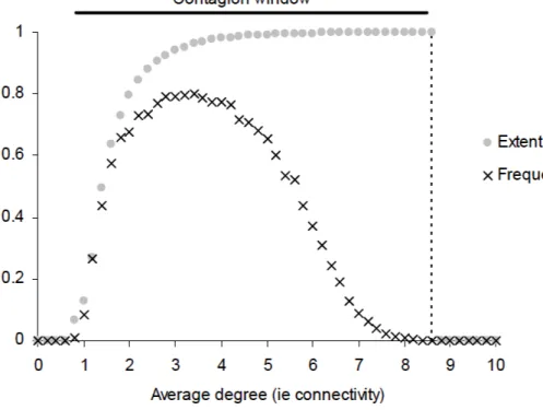
The main finding of the two economists of the Bank of England is that “financial systems exhibit a robust-yet-fragile tendency: while the probability of contagion may be low, the effects can be extremely widespread when problems occur”.
Graphically, this result can be seen in this figure: Indeed we observe that for high
Figure 2.1: Gai Kapadia benchmark model, Chart. 3
degrees of connectivity the frequancy of contagion is very low, but the extent is complete in the system.
Chapter 3
The model
As it has been seen in the previous chapter, almost all the literature on contagion in financial networks has focused its attention primarily on how idiosyncratic ex-ogenous shocks represented by the sudden failure of a bank can affect the financial system.
Due to its nature, the type of shock typically assumed by the majority of the models of this kind, mimics the effects of a fraud event or of a macroeconomic shock with particularly adverse consequences for one institution (see Gai-Kapadia (2010)). Al-though purely idiosyncratic shocks have happened in the past and have led to the failure of some financial institutions (for example Barings Bank, the oldest merchant bank of London, in 1995), they are rare events and not the norm. Therefore, es-pecially form a policy point of view, it would be appropriate to test the resilience of the financial system also on more frequent events, like economic downturns and declines in demand.
Our analysis aims to take a step in this direction, trying to provide a more solid microfoundation for the initial shock. In our model the initial shock is not produced by the default of a bank, but by the default of a certain number of firms, which follows from a fall in aggregate demand that put them out of business and makes them unable to pay back their loans. In other words the we induce an initial real shock at firms level and then we let it propagate to the financial system, with con-sequences that depend of the features of such a system. It is worth noting that in
this way, since more banks can have loans to the same firm and that more firms can have loans with the same bank, we do not have a single “big shock”, but a plurality of “small” shocks hitting different parts of the financial system.
Starting from the work of Gai and Kapadia (Gai & Kapadia, 2010), we developed a model able to asses the probability and the extent of contagion when the initial shock is the one described above.
By contagion we mean the mechanism through which “a shock that initially affects only a particular region or sector or perhaps even a few institutions can become sys-temic and then infect the larger economy” (Allen et al. , 2009).
To preserve the possibility of a comparison with the result provided in Gai and Ka-padia (2010), we manteined, when possible, the same assumptions, for example we will use the same network structure (i.e. a random network) and the same definition of probability of contagion (i.e. the likelihood of defaults hitting at least 5% of the system). However, in order to overcome some of the limits of the original model, we departed from it in several crucial respects, from the already mentioned type of intial shock, to other aspects that will be described in the next section. As final remark it must be said that, for the way in which they are modelled, the nodes rep-resenting firms could also be thought of as reprep-resenting households, since in reality also households can borrow from banks15.
3.1
The logic of the model
The model that we are going to present takes as key starting point the work of Gai & Kapadia (2010) described in the previous chapters. It draws also from Nier et al.(2007) in the kind of analysis developed and from Montagna and Lux (2013) in the study of the dynamics of contagion.
15Indeed the link with the banks is the same both for firms and households. However we didn’t
introduce hoseholds in that way because it would have added little to the analysis. A more significant modelization of hoseholds, which could justify their explicit presence in the model, would require the presence of interactions not only between hoseholds and banks, but also with firms. This would have required the modellization of hoseholds behaviour, which goes beyond the scope of this work and it is left for future studies.
The main contact points with Gai & Kapadia (2010) are the network structure adopted and the way in which shocks are transmitted, since losses are allowed to be either absorbed or amplified along the default cascade. In this sense we differ from the mechanism proposed by Nier et al. (2007), according to which shocks gradually fade away.
As mentioned in earlier section and differently from Gai & Kapadia (2010) and almost all the literature on the topic, with some similarities only with Anand et al. (2013), we intorduce a second type of nodes in the network which represent firms, with the aim of providing a first and very elementary conjunction point between the financial side and the real side of the economy. In addition, while Gai and Kapdia assume perfectly homogeneous banks in terms of size and initial balance sheet composition, which only differ in the number of incoming and outgoing links
16, we assume heterogeneous banks and we draw for each of them the intial value of
total asset from an uniform distibution within a range, from which we then calculate the balance sheet. In doing this we do not change the logic behind the construction of the balance sheet since, as in the Gai and Kapadia model, we “derive” the liability side of the balance sheet from the value of the total assets, in accordance with the idea, recently proposed in a famous bullettin of the Bank of England, that lending creates deposits and not the other way around 17. However, at least for
what concerns the model presented in the next sections, a logic of construction that go in a reverse order (i.e. from the deposits to the assets) would not change the results and the choice is just a matter of which economic theory is considered more correct.
3.1.1
Assumptions
We consider an interbank market populated by n financial entities - banks for short - and m firms. The n banks are linked together by their claims on each other and
16As we will see in the numerical simulations this assumption on homogeneity has important
implication on the frequency and spread of the contagion
are also linked to the m firms by the loans given. Firms are assumed not to lend to banks nor to each other. We have, therefore, a network constituted by two types of nodes: banks, which we will call type-1 nodes, and firms, which we will call type-2 node. The interbank assets and liabilities are respectively represented as incoming and outgoing type-1 links (we can think of an asset as an arrow pointing-in a node and of a liability as an arrow pointing-out) which are directed and weighted by the amount of the asset/liability. The liabilities of firms toward banks are represented as type-2 links directed only from firms to banks and weighted by the amount of the liability.
Following (Nier et al. , 2007), we use the scheme in Figure 3.1 in order to represent the balance sheets of a generic bank.
Figure 3.1: Balance sheet structure
The assets Ai of each bank (i = 1, 2, . . . , n) are partitioned into interbank loans li
and external assets ei:
The liabilities Li of each bank are partitioned into internal borrowing bi, customersˆa
deposits di, and net worth (or equity) ηi:
Li = bi+ di + ηi (3.2)
External assets ei are assumed to be a constant fraction (the same for all banks) of
total assets:
ei = θAi (3.3)
Consequently interbank loans li will be:
li = (1 − θ)Ai (3.4)
The net worth (or equity) ηi is assumed to a be a constant fraction (again the same
for all banks) of total (non risk-weighted) assets:
ηi = γAi (3.5)
In order to be solvent, banks’ difference between total assets and total liabilities must be positive, that is:
ηi ≡ li+ ei− bi− di > 0 (3.6)
If the solvency condition is not respected, bank i becomes insolvent and set into default18: defaulted banks are assumed to default on all their liabilities (i.e. par
condicio creditorum is assumed) and for all the amount (i.e. no partial recovery of the asset is assumed19 20), so the corresponding asset of creditor banks are set equal
18As pointed out both from Montagna and Lux and from Gai and Kapadia it would be possible
to impose a minimal capital requirement, but that “would leave our results qualitatively unchanged as it would just lead to a linear rescaling of the balance sheet” (Montagna & Lux, 2013) p.5
19It would be possible to relax this assumption and allow for a partial recovery, namely that
when a linked bank defaults, the creditor bank does not lose all of its asset held against that bank, but get some fraction of it, for example a share of the remaining assets of the defaulted bank proportional to the weight of creditor’s asset over all other liabilities of the defaulted bank.
20As pointed out by Gai and Kapadia this assumption is likely to be realistic in the middle
to zero and their balance sheets are accordingly reduced by the amount loss.
3.1.2
The algorithm: 1) initializing the model
For each computer simulation we perform the following steps in sequence.
As a first step we draw at random the level of total assets form an uniform disti-bution in a range [Amin, Amax]. We then construct the balance sheet of banks using
equations (4.1), (4.3) - (4.5).
Subsequently, we generate the inter-bank network represented by a (Poisson) random graph in which each possible directed link is present with independent probability p; in the same way we construct the firms-banks network. Hence we have two random graph Γ1(n, p1) and Γ2(n, m, p2), which can be represented mathematically by two
adjacency matrices, an nxn and an nxm matrix. The elements of the matrices are, for the moment, only 0 or 1: a 0 means absence of link; a 1 in the element i, j signals the presence of a link which goes from node j to node i, so it is an incoming link for node i and an outgoing link for node j. The main diagonal of Γ1(n, p1)
has only zeros beacuse self-loops, i.e. links starting and ending in the same node, are not allowed (in other words a bank cannot have a credit or debit with itself); instead, consistently with bankruptcy law, we do not net interbank positions, so two banks can be linked with each other in both directions. Γ2(n, m, p2) is a rectangular
matrix so it hasn’t a main diagonal, however no restrictions on the presence of 1 are imposed.
The algorithm then calculates the number of incoming type-1 links for each node and computes the value of each single interbank asset by dividing the total interbank assets of bank i by its number of incoming links. Therefore all the interbank assets owned by a bank are of the same amount. In the same way we calculate the number of incoming type-2 links for each bank and the value of each single external asset.
will be highly uncertain and banksˆa funders are likely to assume the worst-case scenario.(Gai & Kapadia, 2010). This is what actually happened in the case of Lehman Brothers, where the partial refunds are still not completed after six years. Intuitively, relaxing this assumption will reduce the frequency of contagion and the extent of contagion, but a more carefull study of the effects of a positive rate of recovery are left for future work.
Hence we have that the total interbank asset position and the total external asset position of every bank is evenly distributed over each of its incoming links.
Once found the amount of the average interbank and external asset for each bank, we substitute it, row by row, in the respective adiacency matrices in place of 1, obtaining two matrices weighted for the amount of the assets.
Thus summing along the second dimension of the banks-banks adjacency matrix (i.e. making the column sum), we obtain for each bank the total amount on its in-terbank assets li. In the same way we obtain the total amount on its external assets
ei from the banks-firms adiacency matrix. Moreover, since every interbank asset
is another bankˆas liability, interbank liabilities are endogenously determined in the system, therefore summing along the first dimension of the banks-banks adjacency matrix (i.e. making the row sum), we obtain for each bank the total amount on its interbank liabilities bi.
We further assume that banks with no type-1 incoming links but with type-2 incom-ing links have li = 0 and Ai = ei; banks with type-1 incoming links and no type-2
incoming links have ei = 0 and Ai = li; banks with no type-1 incoming links and no
type-2 incoming links have li = 0, ei = 0 and Ai = 0 (i.e. the bank is removed from
the network).
Finally, exploiting relation (4.2) and (4.6) we fill the liability side of the balance sheet, which is “topped-up” by deposits.
3.1.3
The algorithm: 2) shock trasmission
After the initial shock, banks linked with defaulted firms occur in a loss. If the loss of one or more banks is big enough to overcome its net worth and to make it unable to respect the solvency condition (4.6), then the bank is setted into default and creditors mark down to zero the value of their claim. If the resulting loss for creditors exceeds their net worth, then also creditors are setted into defaults and another round of marksdowns begins. Otherwise if the net worth is sufficient to cushion the loss occurred, net woth is reduced by the amount of the loss, the
bank hitted keeps surviving and the shock is not transimtted to other banks. This mechanism is repeated until no further default occurs.
Therefore the initial shock is allowed both to be absorbed both to be amplified by the system through a series of default cascades which may end up in a systemic crisis.
Chapter 4
Simulations results
To illustrate the results of the model described in the previous chapter, we calibrate it with empirically observed values of the parameters21 and simulate it numerically
in MatLab through Monte Carlo technique. We run 100000 simulation for the bench-mark case and 10000 simulations when we compare the effects of different values of the parameters, because of computational time constraints. Clearly the higher the number of simulations the better are the results: we observed that for 100000 repetitions the results are very good, with 10000 they are more “noisy”, but still good enough to detect the trend of the system.
In each simulation we generate a (Poisson) random graph22, where each node of the
network represents a bank and each possible directed link is present with indepen-dent probability p.
Our algorithm explicitly avoid the possibility of self-loops in the generation of type-1 network (i.e. of links strating and ending in the same node) because it would make no sense to have banks with links (i.e credits and/or debits) with itself; to do so we substitute the ones that may be present on the main diagonal of the randomly generated adjacency matrix with zeros. This implies an ex post change of the
out-21When empirically observed values are not available we usually test a wide range of values;
in the case neither empirical values are used nor wide ranges are explored we will point it out explicitly, explaining the reason why we decide to choose that particular value of a parameter.
22As in Gai and Kapadia, the random graph has been chosen for simplicity and conducting the
simulation analysis under different degree distributions would be a useful extension which we left for future work.
come of the distibution used to generate the network and a difference between the theoretical and actual degree of connectivity. This operation may appear not per-fectly correct from a theoretical point of view, but given the high number of nodes this “bias” is very small and therefore neglegible23. Moreover in a random network
structure, where each node is likely to have other links (in our particular case also many other links) and where each node has on average the same number of links, this change is definitely insignificant. It would have been different, for example, in a scale-free network with preferential attachment, where typically there are few nodes with many links and many nodes with few links, so even though it is an unlikely event, to wipe out a link from a node which has few links can have some effect on the overall network structure and so on the aggregate dynamics of the system. Before proceeding to illustrate the results of the computer simulations, one point de-serves to be highlighted since recurs in all subsequent figures. Indeed, following the definition provided by Gai and Kapadia (2010), the “extent of contagion measures the fraction of banks which default, conditional on contagion over the 5% threshold breaking out” (Gai & Kapadia (2010) p.21). This means that the extent of contagion shown in the plots is the arithmetic average not of all the values of the extent of contagion occurred in each repetition, but only of the values greater than 5%. This has important implications because, in principle, it is possible that on 1000 repeti-tions the extent of contagion is lower than 5% for 999 times and equal to 100% for 1 time. According to the above definition the extent of contagion would therefore be equal to 100%, but trust this measure would be an error because it is flawed by an insufficient statistic: indeed, depending on the specific values of the parameters, for some degrees of connectivity we do not have a sufficiently high level of observations to compute a significative average and we have to compute an average over very few observations.
There are at least two possible solutions to this issue. One is to perform dynamic
23Anyway it would be possible to correct such a distortion by recomputing the actual probabiliy
of the network and using the actual value instead of the theoretical one for calculating the average degree. When the difference between the actual and the theoretical value is small as in our case it is not worth to do that.
simulations, namely to run the simulations until it is reached a significant level of observations for all degrees of connectivity. This option is surely the best solution from a theorical point of view, but it is extremely costly in computational terms. Another solution, which is the one adopted here, is to increase the number of simu-lations to an order of magnitude sufficiently high to get enough observations. This solution is less sound than the previous from a theorical point of view and has the drawback that does not guarantee a priori the desired result, but it is surely more affordable in computational terms.
With this explanation in mind, the reader knows that the “noisy” fluctuations that may appear in some of the following figures have to be related to this issue, espe-cially in the cases in which the number of simulations is 10000.
In what follows we will focus our attention in analyzing both the final outcome of our simulation in terms of frequancy and extent of contagion, both the dynamics of the system, with particluar attention to the number of rounds (or default cascades) occured, to the number of defaults per round and to the loss of wealth - total and for each round - at aggregate level. We will show that, although the model relies on stylised assumptions, it is able to capture the role of diversification on finan-cial stability and the distinction between risk sharing and risk spreading within the financial network.
4.1
The benchmark case
In the financial system, our principal segment of investigation is the one composed by large banks and large firms since, as a matter of fact, they are more involved in risky business, manage bigger volumes of money and are therefore more relevant in terms of potential risk for the whole system. Accordingly, we consider as a benchmark a network of 100 banks and 500 firms: these values, however arbitrary, can be considered reasonable in the light of our previous assumption and of the fact that the number of financial intermediaries in a system depends on how the system is defined and what counts as a financial intermediary ((Gai & Kapadia, 2010) p.20). Clearly a more accurate comparison with empirical data would be desirable, but it would add little to the overall analysis if data on bilateral exposures between banks and between banks and firms are not (publicly) available.
For the benchmark case the internal structure of the nodes (i.e. the balance sheets of the banks) is parametrised adopting the following values: η = 0.04, = 0.2, pF =
0.0002, δ = 0.1. This values have been choosen in order to preserve as much as possible comparability with the work of Gai and Kapadia (2010); moreover, as reported in (Upper, 2007) the value of θ is braodly consistent with the share of interbank assets owed by banks in developed countries, while the value of η is close to the one measured in the british market. Finally the value of the mortality rate of firms δ has been setted equal to the rate registered for the EU in 2010; this value is also broadly consistent with the one registered in Italy in 2007 by ISTAT which was equal to 7,5%. Therefore it appears to be a good approximation of reality and a good benchmark point24.
4.1.1
Extent and frequency of contagion
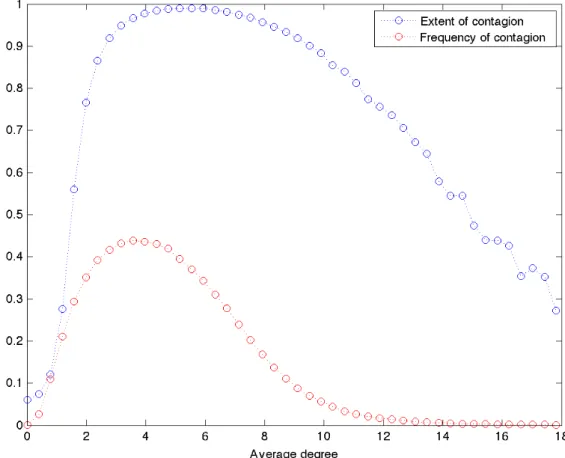
Figure 4.1 shows the extent and the frequency of contagion as a function of the avergage degree computed over T = 100000 repetitions, with θ = 0.2, η = 0.04, pF = 0.0002, δ = 0.1.
Figure 4.1: Extent and frequency of contagion as a function of the avergage degree. In all the 100000 repetitions the other paramenters are fixed at: θ = 0.2, η = 0.04, pF = 0.0002, δ = 0.1
We see that the probability of contagion is non-monotonic in connectivity: it ini-tially increases, peaking above 0.4 when the average degree is between 3 and 5 and then declining toward zero. The extent of contagion is initially increasing very rapidly, reaching its maximum for values of the average degree between 4.4 and 6; then it starts to slowly decreases, but manteining values above 0.9 for a wide range
of average degrees, in particular from values between 3 and almost 1025.
The contagion window, that is the range of average degree for which there is conta-gion above 5% threshold, goes from an average degree of connectivity of 0 to more than 18. The amplitude of the contagion window depends on the heterogeneity be-tween banks’ size: it would have been smaller if we had homogeneous banks (Iori et al. , 2006).
Finally it is possible to note that while high connectivity may reduce the probability of contagion, it can also increase its spread when problems occur, especilly for some ranges of the average degree: in other words crises happens less frequently, but are more severe. We do not find an asymptotic limit (or plateaux) for the extent of con-tagion curve, which shows a maximum for an average degree of 6 and then slowly decreases. This is due to the type of initial shock that we adopted, that is many small shocks at firms level rather that a unique shock at banks level, which is more likely to be absorbed by single banks.
Although the model is very simple and rather mechanical in its working, it is able to capture different features of modern financial systems: the benefits of diversifi-cation deriving from risk sharing (i.e increasing in connectivity) allows to reduce individual risk, but over a certain degree of connectivity they do so at the expenses of the systemic one, because of the risk spreading within the financial network. As a result, idiosyncratic risk is ultimately aggregated and transformed into systemic risk, so that contagion is possible even when diversification of risk in the system is maximised (Gai & Kapadia, 2010).
4.1.2
Dynamic of the model
We now analyze the dynamics of the model considering separately all the results of the simulations and then only the ones in which it has been observed a systemic crisis.
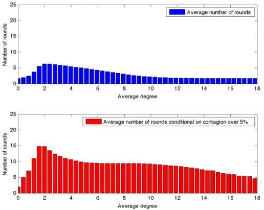
The computer algorithm implemented is albe to track the dynamics of the contagion process trhough the different rounds. In the following two figures we observe the average number of rounds computed on all the simulations performed and average number of rounds computed conditional on contagion.
Figure 4.2: In the top diagram: average number of rounds computed on all the simulations performed. In the bottom diagram: average number of rounds computed conditional on contagion. The results are obtained for θ = 0.2, η = 0.04, pF =
0.0002, δ = 0.1
As we might have expected, the average number of rounds peaks in correspondece of that values of the average degree in which the frequency of contagion is higher.
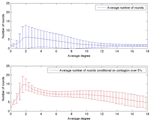
Figure 4.3: In the top diagram: average number of rounds computed on all the simulations performed. In the bottom diagram: average number of rounds com-puted conditional on contagion. In both diagrams vertical bars represent standard deviations. The results are obtained for θ = 0.2, η = 0.04, pF = 0.0002, δ = 0.1
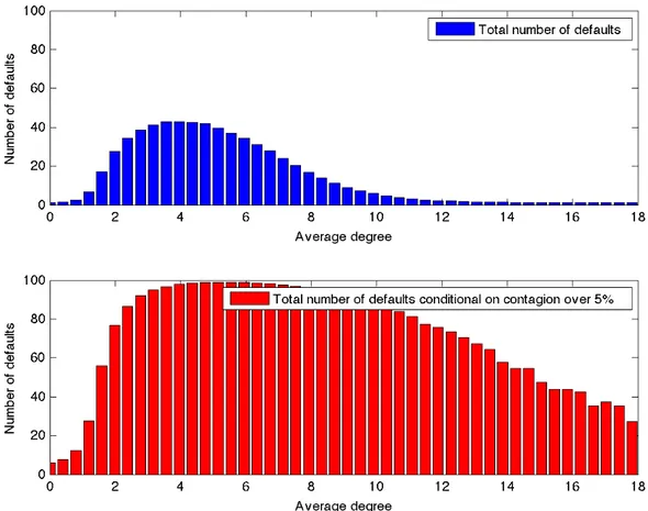
The same obviously holds for the average total number of defaults.
Figure 4.4: In the top diagram: total number of defaults computed as an average of all the simulations performed. In the bottom diagram: average number of rounds computed conditional on contagion. The results are obtained for θ = 0.2, η = 0.04, pF = 0.0002, δ = 0.1
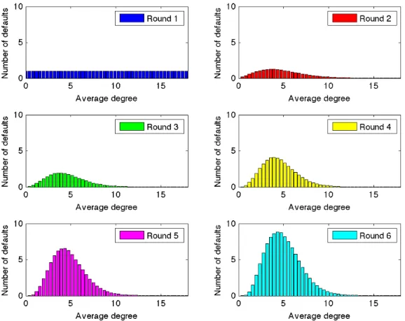
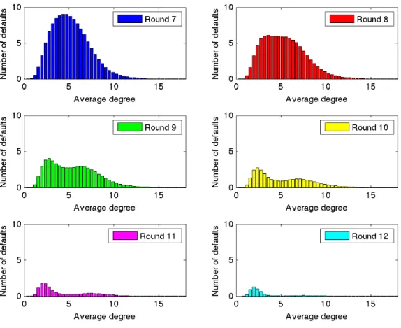
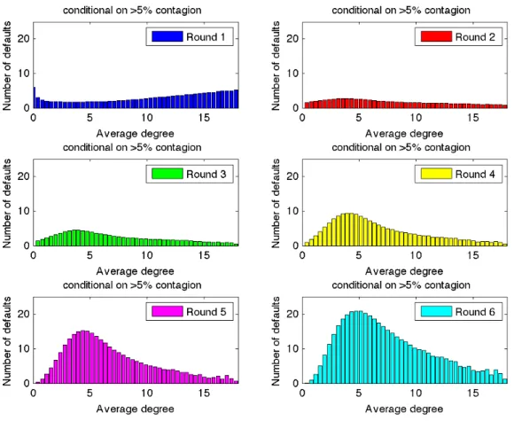
Particularly interesting is how defaults are distributed across different rounds. In-deed, quite surprisingly, when we compute the defaults per rounds we observe an increase in the number of defaults up to round number 7 and then a decrease. This testifies an increasing gravity of the crisis with time, which is the result of a domino effect.
Figure 4.5: The bar plots shows the absolute number of defaults for the first six rounds computed as an average of all the simulations performed. The results are obtained for θ = 0.2, η = 0.04, pF = 0.0002, δ = 0.1
Figure 4.6: The bar plots shows the absolute number of defaults for the second six rounds computed as an average of all the simulations performed. The results are obtained for θ = 0.2, η = 0.04, pF = 0.0002, δ = 0.1
Figure 4.7: The bar plots shows the absolute number of defaults for the first six rounds computed as an average conditional on contagion > 5%. The results are obtained for θ = 0.2, η = 0.04, pF = 0.0002, δ = 0.1
Figure 4.8: The bar plots shows the absolute number of defaults for the second six rounds computed as an average conditional on contagion. The results are obtained for θ = 0.2, η = 0.04, pF = 0.0002, δ = 0.1
The folowing graph shows the aggregate loss in terms of interbank assets as a share on the intial aggregate interbank wealth. Each line corresponds to a different default cascade (i.e. round of defaults) and the area below each line represents the loss occurred during that cascade. We can see that while initial rounds imply a limited aggregate loss, central rounds, namely the ones from the third to the eighth, are those in which the reduction of interbank assets is more severe. This is consistent with the fact that the majority of defaults occur in the middle rounds of cascade as a result of a domino effetc.
Figure 4.9: For each value of the average degree, the graph shows the aggregate loss in terms of interbank assets as a share on the intial aggregate interbank wealth. Each line corresponds to a different default cascade (i.e. round of defaults); the area below each line represents the loss occurred during that cascade. The results are obtained for θ = 0.2, η = 0.04, pF = 0.0002, δ = 0.1
In the following four figures it is shown the aggregate loss disaggregated per round calculated as an average on all the simulations.
Figure 4.10: For every average degree, the plots show the loss associated to the first six rounds. The results are obtained for θ = 0.2, η = 0.04, pF = 0.0002, δ = 0.1
Figure 4.11: For every average degree, the plots show the loss associated to the second six rounds. The results are obtained for θ = 0.2, η = 0.04, pF = 0.0002, δ =
In the following four figures it is shown the aggregate loss disaggregated per round calculated as an average conditional on contagion.
Figure 4.12: For every average degree, the plots show the loss associated to the first six rounds conditional on contagion. The results are obtained for θ = 0.2, η = 0.04, pF = 0.0002, δ = 0.1
Figure 4.13: For every average degree, the plots show the loss associated to the second six rounds conditional on contagion. The results are obtained for θ = 0.2, η = 0.04, pF = 0.0002, δ = 0.1
4.2
Varying η
In the following section we run the model for T = 100000 repetitions for different values of η keeping fixed the others parameters at the values used in the benchmark case, namely θ = 0.2, pF = 0.0002, δ = 0.1.
This exercise allows us to study which are the possible effects of an higher level of net worth.
4.2.1
Extent and frequency of contagion
Testing our model for variuos values of η it turns out that increasing the value of the equity reduces the probability and the extent of contagion because banks have more capital to absorb losses and dampen the shocks.
Indeed, by looking at Figure 14, we see that the probability of contagion switch from about 30% in the case of η = 0.03 to 10% in the case of η = 0.08.
Also the spread of contagion is enormously reduced and passes from 1 at η = 0.03, to 0.4 at η = 0.03. Indeed the y-axis of the subplot (d), (e) and (f) do not reach 1, in other words even if at a first look they may seem not too much different form, for example, subplot (a), indeed they are.
Therefore the increasing in η has the general effect of reducing both the risk of a systemic crise, both its extent, for every level of average degree.
(a) η = 0.02 (b) η = 0.03
(c) η = 0.04 (d) η = 0.05
(e) η = 0.06 (f) η = 0.07
Figure 4.14: Extent and frequency of contagion as a function of the avergage degree. The results are obtained for different values of η, given the values of the other parameters fixed at θ = 0.2, pF = 0.0002, δ = 0.1
4.2.2
Dynamic of the model
As for the benchamrk case we now analyze the dynamics of the model considering separately all the results of the simulations and then only the ones in which it has been observed a systemic crisis.
As η increases the average number of rounds decreases both when computed on all the simulations’ result both when only conditional on contagion.
(a) η = 0.02 (b) η = 0.03
(c) η = 0.04 (d) η = 0.05
(e) η = 0.06 (f) η = 0.07
Figure 4.15: In the top diagram: average number of rounds computed on all the simulations performed. In the bottom diagram: average number of rounds computed conditional on contagion. The results are obtained for different values of η, given the values of the other parameters fixed at θ = 0.2, pF = 0.0002, δ = 0.1
(a) η = 0.02 (b) η = 0.03
(c) η = 0.04 (d) η = 0.05
(e) η = 0.06 (f) η = 0.07
Figure 4.16: In the top diagram: total number of defaults computed as an average on all the simulations performed. In the bottom diagram: average number of rounds computed conditional on contagion. In both diagrams vertical bars represent stan-dard deviations. The results are obtained for different values of η, given the values of the other parameters fixed at θ = 0.2, pF = 0.0002, δ = 0.1
(a) η = 0.02 (b) η = 0.03
(c) η = 0.04 (d) η = 0.05
(e) η = 0.06 (f) η = 0.07
Figure 4.17: In the top diagram: total number of defaults computed as an average of all the simulations performed. In the bottom diagram: average number of rounds computed conditional on contagion. The results are obtained for different values of η, given the values of the other parameters fixed at θ = 0.2, pF = 0.0002, δ = 0.1
The folowing graph shows the aggregate loss in terms of interbank assets as a share on the intial aggregate interbank wealth. Each line corresponds to a different default cascade (i.e. round of defaults) and the area below each line represents the loss occurred during that cascade. It is immediatly clear how an increase in η decreases dramatically the average loss of the system, from a level of 30% with η = 0.02 to less the 5% with η = 0.07. So an increase in η has a positive effect of the stability of the system which is more than proportional. This is due to a positive domino effetc (or virtuos circle) which doesn’t allows losses to spread and cause other losses, reducing (as it has been seen in the previous figures) the average number of defaults, but not the number of rounds. Therefore an intial increase in η, even though may be costly for banks, has potential benefits which far exceeds their cost.
(a) η = 0.02 (b) η = 0.03
(c) η = 0.04 (d) η = 0.05
(e) η = 0.06 (f) η = 0.07
Figure 4.18: For each value of the average degree, the graph shows the aggregate loss in terms of interbank assets as a share on the intial aggregate interbank wealth. Each line corresponds to a different default cascade (i.e. round of defaults); the area below each line represents the loss occurred during that cascade. The results are obtained for different values of η, given the values of the other parameters fixed at θ = 0.2, pF = 0.0002, δ = 0.1
4.3
Varying θ
In the following section we run the model for T = 100000 repetitions for different values of θ keeping fixed the others parameters at the values used in the benchmark case, namely η = 0.04, pF = 0.0002, δ = 0.1.
This exercise allows us to study which are the possible effects of an higher share of external assets in banks’ balance sheets on the whole system.
4.3.1
Extent and frequency of contagion
Testing our model for variuos values of θ it turns out that increasing its level increases enormously the probability and the extent of contagion, also for high degrees of connectivity.
This is due to the fact that higher θ means higher average loans to firms for each bank and therefore also higher losses when a firm default, while η doesn’t increase proportionally because it is a fraction ot total assets of every bank and not of external assets.
(a) θ = 0.1 (b) θ = 0.2
(c) θ = 0.3 (d) θ = 0.4
(e) θ = 0.5 (f) θ = 0.6
Figure 4.19: Extent and frequency of contagion as a function of the avergage degree. The results are obtained for different values of θ, given the values of the other parameters fixed at η = 0.04, pF = 0.0002, δ = 0.1
4.3.2
Dynamic of the model
As for the benchamrk case we analyze the dynamics of the model considering sepa-rately all the results of the simulations and then only the ones in which it has been observed a systemic crisis.
As θ increases the average number of rounds is almost unchanged both when com-puted on all the simulations’ result both when only conditional on contagion.
(a) θ = 0.01 (b) θ = 0.02
(c) θ = 0.03 (d) θ = 0.04
(e) θ = 0.05 (f) θ = 0.06
Figure 4.20: In the top diagram: average number of rounds computed on all the simulations performed. In the bottom diagram: average number of rounds computed conditional on contagion. The results are obtained for different values of θ, given the values of the other parameters fixed at η = 0.04, pF = 0.0002, δ = 0.1
(a) θ = 0.01 (b) θ = 0.02
(c) θ = 0.03 (d) θ = 0.04
(e) θ = 0.05 (f) θ = 0.06
Figure 4.21: In the top diagram: total number of defaults computed as an average on all the simulations performed. In the bottom diagram: average number of rounds computed conditional on contagion. In both diagrams vertical bars represent stan-dard deviations. The results are obtained for different values of θ, given the values of the other parameters fixed at η = 0.04, pF = 0.0002, δ = 0.1
(a) θ = 0.01 (b) θ = 0.02
(c) θ = 0.03 (d) θ = 0.04
(e) θ = 0.05 (f) θ = 0.06
Figure 4.22: In the top diagram: total number of defaults computed as an average of all the simulations performed. In the bottom diagram: average number of rounds computed conditional on contagion. The results are obtained for different values of θ, given the values of the other parameters fixed at η = 0.04, pF = 0.0002, δ = 0.1
The figure in the next page shows the aggregate loss in terms of interbank assets as a share on the intial aggregate interbank wealth. Each line corresponds to a different default cascade (i.e. round of defaults) and the area below each line represents the loss occurred during that cascade.
It is immediatly clear how an increase in θ increases dramatically the average loss of the system, from a level of less than 5% with θ = 0.01 to a level of more than 30% with θ = 0.06.
An increase in θ (given the value of η) has therefore detrimental effect on the stability of the system because, given the assumptions of our model, by increasing the average size of firms present, it ultimately increases the value of the intial loss at aggregate level.
(a) θ = 0.01 (b) θ = 0.02
(c) θ = 0.03 (d) θ = 0.04
(e) θ = 0.05 (f) θ = 0.06
Figure 4.23: For each value of the average degree, the graph shows the aggregate loss in terms of interbank assets as a share on the intial aggregate interbank wealth. Each line corresponds to a different default cascade (i.e. round of defaults); the area below each line represents the loss occurred during that cascade. The results are obtained for different values of θ, given the values of the other parameters fixed at η = 0.04, pF = 0.0002, δ = 0.1
4.4
Varying p
FIn the following section we run the model for T = 100000 repetitions for different values of pF keeping fixed the others parameters at the values used in the benchmark
case, namely η = 0.04, θ = 0.2, δ = 0.1.
This exercise allows us to study which are the possible effects of an higher connec-tivity between banks and firms, namely of more lending acconnec-tivity directed to firms, on the whole system.
4.4.1
Extent and frequency of contagion
Testing our model for variuos values of pF it turns out that increasing its level
increases the probability of contagion, but not its extent (fluctuation of the blue curve for high degrees of connectivity for pF = 0.0001 and pF = 0.0002 are again
due to insufficient observations).
This is due to the fact that more banks can be linked with the same firm and the failure of a firm can put in troubles more banks simultaneously, so increasing the probability of a crisis.
(a) pF = 0.0001 (b) pF = 0.0002
(c) pF = 0.0003 (d) pF = 0.0004
Figure 4.24: Extent and frequency of contagion as a function of the avergage degree. The results are obtained for different values of pF, given the values of the other
4.4.2
Dynamic of the model
As for the benchamrk case we analyze the dynamics of the model considering sepa-rately all the results of the simulations and then only the ones in which it has been observed a systemic crisis.
As pF increases the average number of rounds is almost unchanged both when
com-puted on all the simulations’ result both when only conditional on contagion.
(a) pF = 0.0001 (b) pF = 0.0002
(c) pF = 0.0003 (d) pF = 0.0004
Figure 4.25: In the top diagram: average number of rounds computed on all the simulations performed. In the bottom diagram: average number of rounds computed conditional on contagion. The results are obtained for different values of η, given the values of the other parameters fixed at θ = 0.2, pF = 0.0002, δ = 0.1
The figure in the next page shows the aggregate loss in terms of interbank assets as a share on the intial aggregate interbank wealth. Each line corresponds to a different default cascade (i.e. round of defaults) and the area below each line represents the loss occurred during that cascade.
(a) pF = 0.0001 (b) pF = 0.0002
(c) pF = 0.0003 (d) pF = 0.0004
Figure 4.26: In the top diagram: total number of defaults computed as an average on all the simulations performed. In the bottom diagram: average number of rounds computed conditional on contagion. In both diagrams vertical bars represent stan-dard deviations. The results are obtained for different values of pF, given the values
(a) pF = 0.0001 (b) pF = 0.0002
(c) pF = 0.0003 (d) pF = 0.0004
Figure 4.27: In the top diagram: total number of defaults computed as an average of all the simulations performed. In the bottom diagram: average number of rounds computed conditional on contagion. The results are obtained for different values of pF, given the values of the other parameters fixed at η = 0.04, θ = 0.2, δ = 0.1
An increase in pF increases the average loss of the system, especially for low values
of the average degree.
(a) pF = 0.0001 (b) pF = 0.0002
(c) pF = 0.0003 (d) pF = 0.0004
Figure 4.28: For each value of the average degree, the graph shows the aggregate loss in terms of interbank assets as a share on the intial aggregate interbank wealth. Each line corresponds to a different default cascade (i.e. round of defaults); the area below each line represents the loss occurred during that cascade. The results are obtained for different values of pF, given the values of the other parameters fixed at
4.5
Varying δ
In the following section we run the model for T = 100000 repetitions for different values of δ keeping fixed the others parameters at the values used in the benchmark case, namely η = 0.04, θ = 0.2, pF = 0.0002.
This exercise allows us to study which are the possible effects of different magnitude of initial shocks on the whole system.
4.5.1
Extent and frequency of contagion
(a) δ = 0.05 (b) δ = 0.075
(c) δ = 0.1 (d) δ = 0.125
Figure 4.29: Extent and frequency of contagion as a function of the avergage degree. The results are obtained for different values of δ, given the values of the other parameters fixed at θ = 0.2, η = 0.04, pF = 0.0002
4.5.2
Dynamic of the model
Testing our model for different values of δ it turns out that increasing the number of firms initially set into default implies an increas in the probability, but not much in the extent of contagion.
(a) δ = 0.05 (b) δ = 0.075
(c) δ = 0.1 (d) δ = 0.125
Figure 4.30: In the top diagram: average number of rounds computed on all the simulations performed. In the bottom diagram: average number of rounds computed conditional on contagion. The results are obtained for different values of δ, given the values of the other parameters fixed at θ = 0.2, η = 0.04, pF = 0.0002
The figure in the next page shows the aggregate loss in terms of interbank assets as a share on the intial aggregate interbank wealth. Each line corresponds to a different default cascade (i.e. round of defaults) and the area below each line represents the loss occurred during that cascade.