The effect of marine protected areas of the biological environment. A case of study in southern Sardinia (Capo Carbonara (MPA)

ITALY CAGLIARI

We recommend that the thesis prepared under our supervision by

CORRIAS STEFANO

Entitled

THE EFFECT OF MARINE PROTECTED AREAS ON THE BIOLOGICAL ENVIRONMENT. A CASE OF STUDY IN SOUTHERN SARDINIA

(CAPO CARBONARA MPA)

be accepted in partial fulfilment of the requirements for the degree of

DOCTOR OF PHILOSOPY IN ENVIRONMENTAL SCIENCE AND ENGINEERING

Professor VALAORAS GEORGIA Committee Member

Professor Doctor KASPER JAN Committee Member

Professor FAVA FABIO Committee Member

Professor Doctor CAU ANGELO Advisor

Professor CAO GIACOMO PhD Coordinator

THE EFFECT OF MARINE PROTECTED AREAS ON THE BIOLOGICAL

ENVIRONMENT.

A CASE OF STUDY IN SOUTHERN SARDINIA

The growing interest in environmental issues and the establishment of new protected areas on land and seaside correspond to the worldwide need to understand and preserve the natural development of the ecosystems.

The establishment of protected areas is fairly new for the marine habitat.

It is becoming increasingly clear that marine protected areas represent an effective biodiversity conservation tool. Nowadays, there is a widespread growing need to recognize ecosystem interactions and to improve the effectiveness of protected areas in order to understand biological interrelations and human impacts.

It was the lack of high quality and rigorous monitoring data concerning the marine protected areas (and not the lack of effects, which are almost certain) to bring us to perform the environmental monitoring described in this thesis. In order to understand the biological interactions of a marine protected area in the Mediterranean sea, a study was carried out inside and around the Marine Protected Area of Capo Carbonara located off the southern Sardinia Island. Samplings were performed to identify and quantify the benthonic fish stock and the composition of benthos in rocky shores at different depths and in different times of sampling.

The composition of fish assemblages was evaluated both by the non-destructive visual census with SCUBA technique and the non-destructive method of the trammel net fishing.

Sciaenidae, Scorpaenidae, Serranidae, Sparidae, Sphiraenidae).

The fish assemblages observed inside the protected area and outside, in the unprotected fished area were statistically different during all the sampling periods. Larger amount of fish was found in the protected than in the fished area, and differences were observed in total fish density, abundance, biomass: most fish species targeted by fisheries had a greater density (e.g.

Diplodus puntazzo, Diplodus sargus, Diplodus vulgaris, Epinephelus marginatus, Mullus surmuletus, Pagrus pagrus, Sciena umbra, Scorpaena porcus, Serranus scriba, Sphyraena Sphyraena and Synphodus tinca) and/or

size (e.g. Dentex dentex, Diplodus puntazzo, Diplodus sargus) within the protected area than in the fished areas outside.

In the internal protected areas the Shannon Weaver diversity index showed richer ichtiofauna than outside, near the boundaries.

Cluster analysis and MDS plot showed a general progressive increased similarity between protected and unprotected sites from the early census to the end, validating the spillover effects from inside to outside areas. These results indicate that reserve effects (protection) from fishing may have the potential to influence fish assemblages of outside areas.

The composition of benthos in hard substrate, was examined applying benthic biocoenosis census through photographic and SCUBA techniques.

Three years of sampling displayed the usefulness of the used techniques in a low budget study.

The Visual census outcomes for macro benthic biocoenosis assemblages (5-25 m deep), assessed from September 2004 to May 2006, revealed 3(5-25

in all the analyzed sites.

The analysis of the community structure revealed high biodiversity. In each sampling an ecological index classification as “Moderate” was recorded, both in the whole sanctuary and nearby the boundaries. In particular, some sites within the sanctuary showed a “Good” quality in different times and at different depths.

Moreover, ecological and environmental factors able to modify the benthic composition often risked to warp outputs e.g. the presence of an alien species, the Caulerpa racemosa. In particular the analysis of these green algae within the sites was necessary because of its influence on the environment and consequently on the statistical analysis outputs.

It is relevant that the recorded temporal scale of events can be useful for further analysis in the studied area and/or in other Marine Protected Areas. The application of this protocol seems to be a functional tool to manage marine environments almost until a co-ordinated network between the Mediterranean Marine Protected Areas will be created.

ACKNOWLEDGEMENTS

First of all, I would like to thank my advisor Professor Dr. Angelo Cau for his

guidance and support throughout my graduate studies. Without the numerous

discussions and brainstorms with him, the results presented in this thesis

would never have existed. I am grateful to Dr. Piero Addis, for his valuable

comments and suggestions on my research. I thank Professor Dr. Anna Maria

Deiana and Dr. Danila Cuccu for their help during my collaboration with the

Department of Animal Biology and Ecology of Cagliari.

Last but not least, I would like to thank my wife and my little children for their

constant love and support. It would be impossible for me to express my

ABSTRACT... i

ACKNOWLEDGEMENTS... iv

LIST OF TABLES...vii

LIST OF FIGURES ...vii

1 INTRODUCTION... 1

1.1 WHAT MARINE PROTECTED AREAS ARE ... 1

1.2 MARINE PROTECTED AREAS IN THE MEDITERRANEAN SEA... 3

1.3 STUDY DESIGN... 5

1.4 THE MARINE PROTECTED AREA OF CAPO CARBONARA ... 7

1.5 INVESTIGATED SITES ... 13

1.5.1 CAPO CARBONARA ... 13

1.5.2 ISOLA DEI CAVOLI... 14

1.5.3 ISOLA DI SERPENTARA... 15

1.5.4 PUNTA IS PROCEDDUS... 16

1.5.5 CALA PIRA... 16

1.5.6 SOLANAS – CAPO BOI ... 17

1.5.7 TORRE DELLE STELLE ... 18

2 FISH FAUNA ANALYSIS ... 19

2.1 VISUAL CENSUS ... 23

2.2 VISUAL CENSUS TECHNIQUE... 24

2.2 1 DATA COLLECTION... 24

2.2 2 SAMPLING PROCEDURE... 24

2.2.2.a TIMING OF CENSUS ... 26

2.2.2.b DATA RECORDING... 26

2.2.3 DATA MANAGEMENT ... 27

2.2.4 STATUS OF FISH STOCKS ... 29

A) Identifying and counting species ... 29

B) Counting individuals ... 29

C) Statistical analysis ... 31

2.2.5 SOURCES OF ERROR... 35

2.3 SAMPLING DESIGN ... 42

2.4 RESULTS AND DISCUSSION ... 46

3 TRAMMEL NET FISHING ... 60

3. 1 FISHING TECHNIQUES... 62

3 1.1 STATUS OF FISH STOCKS ... 63

3.2 MATERIALS AND METHODS... 64

3 2.1 SAMPLING TIME ... 64

3 2.2 SAMPLING DESIGN ... 64

3.3 RESULTS AND DISCUSSION ... 65

4 MACRO BENTHIC BIOCOENOSIS CENSUS ... 73

4.1 PHOTOGRAPHIC TECHNIQUE ... 74

4.1.1 DATA COLLECTION... 75

4 1.2 SAMPLING PROCEDURE... 75

4.1.3 DATA ANALYSIS ... 75

4.1.4 THE ECOLOGICAL STATUS AND ECOLOGICAL EVALUATION INDEX ... 79

4.2 MATERIALS AND METHODS... 85

4.2.1 TIME SAMPLING ... 85

4.2.2 SAMPLING DESIGN ... 86

A) IN FIELD PROCEDURES ... 88

B) PICTURES MANAGEMENT... 89

4.3 RESULTS AND DISCUSSION ... 93

4.3.1 ANALYSIS OF THE COMMUNITY STRUCTURE ... 95

BIBLIOGRAPHY... 132

APPENDIX 1: Anthropogenic stress on marine benthic macrophytic communities. ... 146

APPENDIX 2: Functional characteristics and growth strategies of marine benthic macrophytes. ... 147

APPENDIX 3: Check list of studied Macro Phytobenthos in the MPA... 148

APPENDIX 4. Check list of studied Macro Zoobenthos in the MPA ... 152

APPENDIX 5: Check list of studied fish species in Capo Carbonara MPA. ... 157

APPENDIX 6: Fish visual census biomass per specimen (mean)... 158

Table 1.1: Boundaries of the MPA. ... 12

Table 2.1: Summary of the different sampling methods... 21

Table 2.2: Summary table... 30

Table 2.3: Sources of error... 35

Table 2.3: Latitude and longitude of the sampling sites... 44

Table 2.4: Fish visual census; target species. ... 44

Table 2.5: The 24 target species occurred in the three sampling Sites. ... 46

Table 3.1: Trammel net fishing: species occurred in the three sampling zones... 65

Table 4.1: Matrix for the evaluation of the Ecological State Class ... 83

Table 4.3: Numerical scoring system for the evaluation of ecological status... 85

Table 4.4: Position of the sampled area. ... 86

Table 4.5: list of the acronyms used for the classification... 91

Table 4.6: Recorded Phyla. ... 94

LIST OF FIGURES Figure 1.1: Marine Protected Areas in the Mediterranean Sea... 4

Figure 1.2: Location of the Marine Protected Area... 7

Figure 1.3-1.4: Partition and view of the sanctuary from Capo Boi boundary. ... 8

Figure 1.5: A zone boundaries... 10

Figure 1.6 - B and C Zone boundaries. ... 11

Figures 1.7-1.8: Capo Carbonara and shoals of Diplodus vulgaris. ... 13

Figures 1.9-1.10-1.11-1.12-1.13: Isola dei Cavoli, the lighthouse, a specimen of Paramuricea clavata and the Serranidae Epinephelus marginatus... 14

Figures 1.14-1.15-1.16-1.17: A specimen of Helicodiceros muscivorus, eggs of sea-gull, a view of the Island and the Anthozoa Parazoanthus axinellae... 15

Figure 1.18: A view of Punta is Proceddus. ... 16

Figure 1.19: The beach of Cala Pira. ... 16

Figures 1.20-1.21: The tower of Capo Boi and the promontory of Torre delle Stelle, the Crustacean Maja squinado... 17

Figures 1.22–1.23: Gerardia savaglia and the world war II shipwreck Isonzo at 48 meters of depth. ... 18

Figure 2.1: Spillover trend from MPA to surrounding areas. ... 19

Figure 2.2: General scheme of visual census survey. ... 25

Figure 2.3: The input mask... 28

Figure 2.4: Sampling sites... 42

Figure 2.5: Fish visual census, distances by the center of the core zone... 43

Figure 2.5: Example of recorded data... 45

Graph 2.1: Total mean weight from the Core Zone (A, North and South), Inside Zone (I, North and South) to Outside of the boundaries (O, North and South); all weight are listed by Time of sampling (Time 1-2-3)... 47

Graph 2.2: Mean length of the target species. ... 48

Graph 2.3: Mean abundance of the species (in number). ... 49

Graph 2.4: Abundance of species in the sampled areas. ... 50

Graph 2.5: Trend of the diversity from the A Zone to Outside South and North... 51

Graph 2.6: Diversity index from 2,1 to 2,6 in the studied areas. ... 52

Graph 2.7: Evenness is nearly one in the site 02N (Punta is Proceddus)... 53

Graph 2.8: High values of Simpson diversity in all the sites and higher from the centre to the Northern sites. ... 54

Graphs 2.9-2.10-2.11: Cluster analysis. ... 56

Figure 3.6: Trammel net fishing Sampling design... 64

Graph 3.1: Mean lenght of the species. ... 66

Graph 3.2: Species increase from Time 1 to Time 2 outside the sanctuary. ... 67

Graph 3.3: Specimen increase from Time 1 to Time 2 both inside and outside... 68

Graph 3.4: Diversity increases from Time 1 to Time 2 both inside and outside. ... 69

Graph 3.5: Index of diversity increases from Time 1 to Time 2 both inside and outside. ... 70

Graph 3.6: Evenness increases from Time 1 to Time 2 Inside and decreases Outside. 70 Graphs 3.7-3.8: Cluster analysis’ and Multidimensional analysis sorted by Time. ... 71

Figure 4.1: Sampled sites: P0 in A Zone, C1 and C2 in B Zone, C3 Outside near the Boundaries and C4 Outside. ... 86

Figure 4.2: Researcher (myself) using the camera equiped with frame and flashes to record the studied substrata... 88

Figure 4.3: The grid subdividing the picture in 25 rectangles, each corresponding to 4 % of the whole image... 89

Figure 4.4: Spirastrella cuntactrix, an uncountable species and countable species like Polychaeta. ... 90

Figure 4.5: Table of the registered data... 92

Figure 4.6: Table of the registered species subdivided by taxonomic rank... 92

Figure 4.7: Table of the interactive database. ... 93

Graph 4.1: Abundance of species in the studied sites: Protection A, B and C and Control 1, 2, 3 and 4. ... 95

Graph 4.2: Number of species subdivided by Time and depth. ... 95

Graphs 4.3 – 4.4: Multi dimensional scaling and cluster analysis of the sampled sites.96 Graph 4.5: Only in Control 3, placed outside near the boundaries (Capo Boi), richness in species was lower than in the other sites. ... 97

Graph 4.6: Degree of evenness was higher in Controls 1 and 2 (I Faraglioni and i Congressi – Isola dei Cavoli) than in other Studied sites... 97

Graph 4.7: Evenness had higher values in controls C1 (I Faraglioni) and C2 (I Congressi) than in protected sites and in other controls... 98

Graph 4.8: higher Diversity in Control 1 and 2, lower in the other sites. ... 99

Graph 4.9: Multidimensional Scaling by site factor... 100

Graph 4.10: Ecological evaluation index for the A zone in the Isola di Serpentara subdivided by Time and depth. ... 106

Graph 4.11: Ecological evaluation index for the B zone in the controls of the Isola dei Cavoli (I Faraglioni and the rocky islet I Congressi) subdivided by Time and depth. .. 107

Graph 4.12: Ecological evaluation index for the C zone in Capo Boi and Torre delle Stelle subdivided by Time and depth... 108

Graphs 4.13 4.14: Cluster analysis and Multidimensional scaling for the Ecological evaluation index in the analyzed sites... 109

Figure 4.8: Ship on the roadstead in the Gulf of Cagliari. ... 111

Figure 4.9: Stolon and erect part of Caulerpa racemosa on hard substrate. ... 114

Figures 4.10 - 4.11: Caulerpa racemosa ... 115

Figure 4.12: The studied area: the same sites examined for macro benthic analysis.. 116

Graph 4.15: Percentage values of Caulerpa racemosa in protected and control sites. 117 Graphs 4.16-4.17- 4.18: Recorded values of Caulerpa racemosa in Site A of the A Zone (Isola di Serpentara), subdivided by depth. ... 118

Graph 4.19- 4.20.- 4.21: Recorded values of Caulerpa racemosa in in Site B of the A Zone (Isola di Serpentara), subdivided by depth... 119

Graphs 4.22- 4.23- 4.24: Recorded values of Caulerpa racemosa in in Site C of the A Zone (Isola di Serpentara), subdivided by depth... 120

Graphs 4.25 - 4.26 - 4.27: Recorded values of Caulerpa racemosa in in Control 1 of the B Zone of the Isola dei Cavoli (I Faraglioni), subdivided by depth. ... 121

Graphs 4.28-4.29-4.30: Recorded values of Caulerpa racemosa in in Control 2 of the B Zone of the Isola dei Cavoli (I Congressi), subdivided by depth. ... 122

sanctuary at Torre delle Stelle, subdivided by depth... 124 Graph 4.37: Recorded values of Caulerpa racemosa showed in multidimensional scaling for protected sites in A Zone (Isola di Serpentara). ... 125 Graph 4.38: Recorded values of Caulerpa racemosa showed in multidimensional scaling for control sites... 126

A1S Sampling Sites (see figure 2.4) AC Articulated Corallinacea C1 Sampling Sites (see figure 4.1) C2 Sampling Sites (see figure 4.1) C3 Sampling Sites (see figure 4.1) C4 Sampling Sites (see figure 4.1) CBD Convention on Biological Diversity

CoNISMa Consorzio Nazionale Interuniversitario Scienze del Mare DFA Dark Filamentous Algae

DM Decreto Ministeriale EB Encrusting Bryozoans ECR Encrusting calcified Rhodophytae ECR Encrusting Calcified Rhodophytae EEI Ecological Evaluation Index ERS Encrusting Red Sponges ESC Ecological State Class ESG Ecological State Group GFA Green filamentous algae GFA Green Filamentous Algae GU Gazzetta Ufficiale

ICRAM Istituto Centrale per la ricerca Applicata al Mare I1N Sampling Sites (see figure 2.4)

I1S Sampling Sites (see figure 2.4) I2N Sampling Sites (see figure 2.4) I2S Sampling Sites (see figure 2.4) ISO International Standards Organization

IUCN International Union for the Conservation of Nature MBBC Macro Benthic Biocoenosis Census

MDS Multi Dimensional Scaling MDS Massive Dark Sponges MPA Marine Protected Area

NGO Non-Governmental Organisation O1N Sampling Sites (see figure 2.4)

O1S Sampling Sites (see figure 2.4) O2N Sampling Sites (see figure 2.4) O2S Sampling Sites (see figure 2.4) O3N Sampling Sites (see figure 2.4) O3S Sampling Sites (see figure 2.4) O4N Sampling Sites (see figure 2.4) O4S Sampling Sites (see figure 2.4) O5N Sampling Sites (see figure 2.4) O5S Sampling Sites (see figure 2.4) O6N Sampling Sites (see figure 2.4) O6S Sampling Sites (see figure 2.4)

OECD Organisation for Economic Co-operation and Development P0A Sampling Sites (see figure 4.1)

P0B Sampling Sites (see figure 4.1) P0C Sampling Sites (see figure 4.1) SBA Soft Branched Algae

SCUBA Self-Contained Underwater Breathing Apparatus TNF Trammel Net Fishing

TRB Thin Ramified Bryozoans TTS Thin Tubular Sheet-like UFVC Underwater Fish Visual Census

WFD Water Framework Directive

W

out of mind,’ that can no longer be the case. Let us work together: to protect the oceans and coastal zones; to help small islands survive and prosper; and to ensure that all people enjoy a sustainable future.

United Nations Secretary General Kofi Annan, 13 January 2005, at the Mauritius International Meeting for Small Island Developing States.

1 INTRODUCTION

1.1 WHAT MARINE PROTECTED AREAS ARE

The marine and coastal areas are critical to the health and more in general to people and communities living nearby.

Healthy waters abound with life providing food, jobs and income. Shallow waters and their ecosystems sustain fisheries which can support regional incomes, coastal trades and traditional culture.

The biological diversity of marine systems is rapidly diminishing all over the world, endangered by over-fishing, loss of habitats due to destructive fishing techniques and inappropriate coastal development, pollution, invasions of alien species which change the natural ecological balance. The long-term threat of climate change, whose influence can already be observed in biologic invasion, changing currents and increasingly violent and destructive storms around the world, overrides all the above mentioned threats.

Marine Protected Areas, in their multitude of forms and sizes, are seen as one of the solutions to cope threats facing the coastal marine sphere. Marine Protected Areas are considered a sustainable development tool contributing to the long term incomes of nearby citizens, to their culture and prosperity. These benefits include enhanced productivity from well managed coastal zones, shoals, beds of sea grass and seaweed, natural protection from wave erosion, increased recreational and tourist chances, as well as greater opportunities for education and research, especially about natural processes in ‘pristine’ regions (investing in the future through the long-term benefits of education).

The international community has recognised the potential role and benefits of Marine Protected Areas (MPAs). The main future goal must be to build representative networks of marine and coastal protected areas.

This is an actually global challenge that can only be realised through committed and effective cooperation.

MPAs are not considered anymore just a conservation tool, but a development and health tool.

The term MPA covers a wide range of different approaches for the management of coastal and marine areas. An MPA as defined by the IUCN is “any defined area within or adjacent to the marine environment, together with its overlying waters and associated flora, fauna, and historical and cultural features, which has been reserved by legislation or other effective means, including custom, with the effect that its marine and/or coastal biodiversity enjoys a higher level of protection than its surroundings.

In this definition, MPAs may include areas managed by governments, local communities, NGOs, development projects or any combination of these or other stakeholders including the private sector.

Many different terms have been used to describe MPAs, including ‘reserves’, ‘closed areas’, ‘no-take zones’, ‘sanctuaries’, ‘parks’ and ‘locally managed areas’. Much of the recent discussion has focused on ‘no-take MPAs’ intended to prohibit all extractive activities and thereby to sustain fisheries production in surrounding waters through “spillover” of fish stocks.

The success or sustainability of many MPAs comes from the collaborative planning with resource users to ensure managed access for each main

stakeholder group, and from a community involvement in governance, so as to promote agreement and support.

Nowadays Mediterranean biodiversity is undergoing rapid alteration under the combined pressure of climate change and human impacts.

1.2 MARINE PROTECTED AREAS IN THE MEDITERRANEAN SEA.

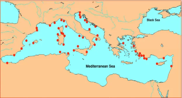
Mediterranean marine biodiversity has received only a fraction of the attention accorded to its terrestrial counterpart, despite the great cultural and economic importance that the sea has been having for the Mediterranean countries (Bianchi N. and Morri C., 2000). At a rough estimate, more than 8.500 species of macroscopic marine organisms should live in the Mediterranean Sea, corresponding to somewhat between 4% and 18% of the world marine species. These data are even more relevant if we consider that the Mediterranean Sea is only 0.82% in surface area and 0.32% in volume compared with the world ocean. The high biodiversity of the Mediterranean Sea may be explained by historical reasons (its tradition of studies) dates older than almost any other sea), paleogeographic reasons (its tormented geological history through the last 5 my has been determining the occurrence of distinct biogeographic categories), and ecological reasons (its variety of climatic and hydrologic situations within a single basin). Figure 1.1 below, shows the 48 MPAs existing in 2003.

Nowadays, there is not a co-ordinated network between the MPAs in the Mediterranean sea, useful tool to implement strategies for the environment conservation and for the economy of the nearby citizens.

Figure 1.1: Marine Protected Areas in the Mediterranean Sea, December 2003 (Rais C., 2003), Modified.

1.3 STUDY DESIGN

The main objective of the present thesis is to understand the role and patterns of marine biodiversity within a Marine Protected Area of Sardinia; to demonstrate that MPAs increase biodiversity in comparison with non-protected marine areas, and to demonstrate the spillover effects that may occur.

The research assessed the evolution of marine environment and the MPAs influences inside and outside, by studying fish fauna in rocky shores and benthos in hard substrates.

For this purpose, a set of samplings was carried out within and outside the MPA.

The biological analysis were subdivided in two main groups: 1. The analysis of fish fauna using:

a. visual census techniques and b. trammel net fishing

2. The analysis of flora using the macro benthic biocoenosis census. Analysis of fish fauna was performed by divers using SCUBA (Self-Contained

Underwater Breathing Apparatus) techniques inside and just outside the

sanctuary analyzing fish abundance, fish biomass and fish length data; trammel net fishing was a fishing technique performed with a boat and nets. The analysis of flora was performed mapping benthic biocoenosis (all the interacting organisms living together) inside and just outside the MPA on hard substrates and estimating the composition with photographic census techniques.

The increased coverage of an alien green alga, the Caulerpa racemosa and its dangerous effects on the environment were the subject of an entire study carried in the analyzed area. This study is presented in the section 4.4 of this thesis.

1.4

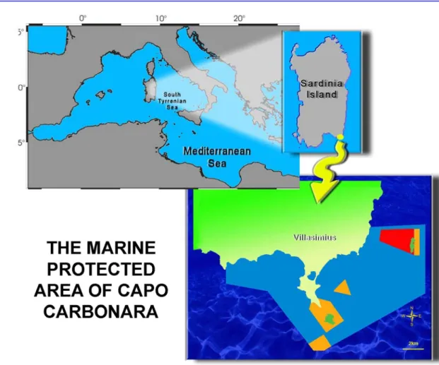
The Marine Area of Capo Carbonara is located in the southern Tyrrenian sea, off the south-eastern coast of Sardinia.

The MPA named as Capo Carbonara – Villasimius, has been instituted in 1988.

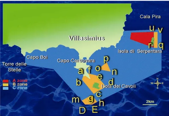
It measures 8857 hectares in surface and 32 km of coastlines which include granitic cliffs. The Area extends from the cape called "Capo Boi" to Cape "Punta Is Proceddus" including the island of Cavoli and Serpentara.

Figure 1.3-1.4: Partition and view of the sanctuary from Capo Boi boundary.

Latitude Longitude A 39° 07' .54 N 009° 26' .47 E B 39° 06' .54 N 009° 26' .47 E C 39° 05' .62 N 009° 28' .49 E D 39° 03' .37 N 009° 31' .40 E E 39° 03' .37 N 009° 32' .05 E F 39° 07' .40 N 009° 37' .19 E G 39° 09' .50 N 009° 37' .19 E H 39° 09' .13 N 009° 34' .13 E MPA boundaries

CHRONOLOGICAL HISTORY OF THE MPA

™ 1991 Identified as a "Area Marina di Reperimento" (National Low L.n.394–1991).

™ 1998 Established with the original institutive Law (D.M. 15.09.1998). ™ 1999 Modified by the D.M. of 03.08.1999 (G.U. n. 229 del 29.09.1999). ™ In progress: Certification ISO 9001.

GENERAL RULES

The regulations in force inside the entire MPA:

• Do not hunt, capture, pick, damage; in general, it is not allowed any activity provoking danger or disturb towards animal and vegetal species, including foreign species intake;

• Do not alter by any mean, directly or indirectly, the geophysical environment and the biochemical features of water; do not dump liquid and solid waste; do not introduce the inlet of any substances which could modify, even temporarily, the characteristics of the marine environment;

• Do not transport arms, explosive materials, destructive and rapture means, toxic and polluting substances.

• Do not practise any activity disturbing or hindering study programs and scientific research.

ADDITIONAL RULES

A ZONE: Primary Reserve, West Area of Isola di Serpentara.

Forbidden: removing, even partially, and damaging geological and mineral formations; navigation, admittance and stops for any ship and yacht; professional and sporting fishing; underwater fishing.

Figure 1.5: A zone boundaries.

Allowed: admittance of personnel of the Administrator Authority for active service; previously licensed scientific researchers; diving previously licensed by Administrator Authority for scientific purposes and submerged sightseeing regulated by the same authority in limited areas and according to previously agreed upon routes.

B ZONE: General Reserve, East Area of Isola di Serpentara, Secca dei Berni, Isola dei Cavoli-Capo Carbonara, South Area of Isola dei Cavoli.

Latitude Longitude r 39° 07' .83 N 009° 36' .43 E r 39° 08' .78 N 009° 34' .76 E t 39° 09' .18 N 009° 34' .76 E u 39° 09' .18 N 009° 36' .46 E

Figure 1.6 - B and C Zone boundaries.

Forbidden: free anchorage; free engine navigation; mooring; underwater fishing.

Allowed: crafts and reduced speed boats navigation (not more than 10 Knots) according to Administrator Authority; professional and sporting fishing previously licensed by the Administrator Authority; mooring to the structures set by the Administrator's Authority; diving, previously licensed.

C ZONE: Partial Reserve, all the other areas in the MPA. Forbidden: free anchorage; mooring; underwater fishing;

Allowed: anchorage where equipped and signalled by the Administrator Authority; crafts and boats navigation; regulated mooring; professional fishing for fishers resident in the town of Villasimius and for those not resident but

licensed by the Administrator Authority as for fishing strain and implements; diving with Administrator permission.

Underwater fishing is forbidden in all the MPA, without differences between Zone A-B-C.

It is also forbidden to anchor your boat in the area where the "Posidonia

oceanica" grows.

East sector of Isola di Serpentara Secca dei Berni

r 39° 07' .83 N 009° 36' .43 E n 39° 06' .47 N 009° 33' .31 E q 39° 07' .83 N 009° 36' .84 E o 39° 06' .70 N 009° 32' .25 E v 39° 09' .33 N 009° 36' .84 E p 39° 07' .29 N 009° 33' .06 E u 39° 09' .18 N 009° 36' .46 E u 39° 09' .18 N 009° 36' .46 E

Isola dei Cavoli - Capo Carbonara South sector of isola dei Cavoli

a 39° 06' .29 N 009° 30' .62 E g 39° 04' .12 N 009° 31' .88 E b 39° 05' .39 N 009° 30' .30 E h 39° 03' .72 N 009° 32' .47 E c 39° 04' .08 N 009° 31' .94 E E 39° 03' .37 N 009° 32' .05 E d 39° 04' .92 N 009° 33' .10 E D 39° 03' .37 N 009° 31' .40 E e 39° 05' .95 N 009° 31' .87 E e 39° 05' .95 N 009° 31' .87 E f 39° 06' .05 N 009° 31' .28 E m 39° 03' .37 N 009° 31' .13 E

1.5 INVESTIGATED SITES

1.5.1 CAPO CARBONARA

The MPA takes its name from the promontory of Capo Carbonara. It is located in the B zone and it is the last tongue of land in South East Sardinia. It is a watershed dividing the South East coast from the East coast.

Shoals start from 0 to 22 meters in the channel between the promontory and the Isola dei Cavoli. Here, shoals of juveniles Diplodus vulgaris can be seen.

Figures 1.7-1.8: Capo Carbonara and shoals of Diplodus

1.5.2 ISOLA DEI CAVOLI

Isola dei Cavoli is in the B zone of the sanctuary. It takes its name from the “Cavorus”, which means crabs in Sardinian language.

Figures 1.9-1.10-1.11-1.12-1.13: Isola dei Cavoli, the lighthouse, a specimen of

Paramuricea clavata and the Serranidae Epinephelus marginatus.

This is the most beautiful Island in the sanctuary, where waters are deep and shoals have depth from 0 to 50 metres and more. These waters are full of life and divers are present all year long.

1.5.3 ISOLA DI SERPENTARA

This is another gorgeous island entirely located in the no take zone (A zone). It is notable for its terrestrial endemic flora and fauna. Here flourishes the

Helicodiceros muscivorus (L. fil.) Engler (figure 1.14).

Figures 1.14-1.15-1.16-1.17: A specimen of Helicodiceros muscivorus, eggs of sea-gull, a view of the Island and the Anthozoa

Parazoanthus axinellae.

This Island is the sanctuary of birds, where their reproductive cycle can take place.

Waters, like the Isola dei Cavoli, are deep and shoals start from 0 to 50 metres.

1.5.4 PUNTA IS PROCEDDUS

Punta Is Proceddus, located in the northern boundary of the C Zone, is characterized by shallow shoals starting from 0 to 17 metres.

Figure 1.18: A view of Punta is Proceddus.

1.5.5 CALA PIRA

Cala Pira is a site situated outside the sanctuary (600 m North direction).

1.5.6 SOLANAS – CAPO BOI

Solanas is a place outside, located near the boundaries in the South West side of the MPA.

Granitic cliffs start on land and end at 25 meters of depth.

Figures 1.20-1.21: The tower of Capo Boi and the promontory of Torre delle Stelle, the Crustacean Maja

squinado.

This site outside the sanctuary, but nearby the West boundary is rich in species of the Crustacean class, like the Maja squinado.

1.5.7 TORRE DELLE STELLE

In the last site, at Torre delle Stelle, there are lots of different environments; in fact in front of the beach of Genn’è Mari there is one of the most beautiful shoals starting from 10 to 40 meters. Here is present the unique specimen of Cnidaria Gerardia savaglia at 27 metres of depth.

Figures 1.22–1.23: The very rare species Gerardia savaglia and the world war II shipwreck Isonzo at 48 meters of depth.

In proximity three shipwrecks from 10 to 67 metres are substrata for different species of flora and fauna.

2 FISH FAUNA ANALYSIS

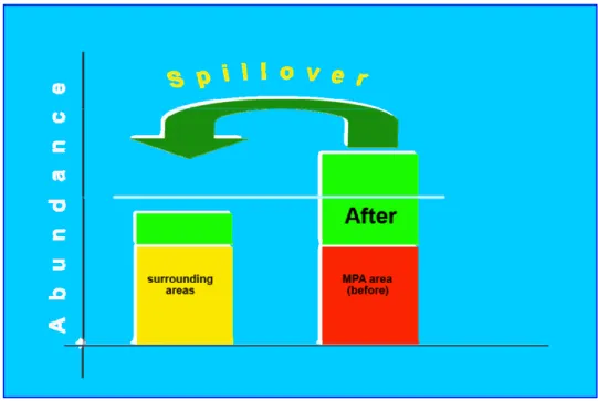
Many studies indicate that MPAs can improve fish stock inside and supply larval and adult fish biomass to adjacent areas (through spillover), helping therefore the enhancement of the surrounding fishery (Halpern and Warner, 2002; Halpern, 2003).

Pioneering works (Russ G. & Alcala A., 1996; Alcala A., 1999) in Apo Island (central Philippines) provided some early evidence that spillover of adult fish biomass from the reserve to fished areas occurs.

Figure 2.1: Spillover trend from MPA to surrounding areas.

A study by Rodwell et al., (2002) in the Mombasa Marine National Park shows, through simulation, that full protection leads to an increase in total fish biomass, and that movement of adult and larval fish from the MPA will increase total fishery catch in surrounding areas. Studies that measure actual yield enhancement from MPA are few (Roberts C. M. et al., 1999), and fewer still deal with valuation of economic benefits from protection.

One of the best ways to demonstrate that the marine reserve helps to sustain a profitable coastal fishery, is to determine whether or not the fishery generates economic or resource rent (surplus value after all costs and normal returns have been accounted for).

The present study is at the beginning in the area of Capo Carbonara. There was only another study called “Afrodite” Project, a national project started in 2003 and ended in 2004, developed by the Environment Ministry, the ICRAM and CoNISMa; now it is the subject of many investigations in other MPAs as a way to evaluate their efficacy in enhancing the fishery in surrounding areas. Many methods exist to measure resources along rocky shores and lagoon: none is perfect and all have advantages and disadvantages. They all share the characteristic of studying a section or subgroup of the population in question. For this reason, they require the use of sampling techniques, which can be divided into three categories:

□ capture methods; □ mixed methods; □ non-capture methods.

Capture methods mainly involve recording information on fish captured in traps (and, more generally, with bait), in nets by trawling, and with lines. These methods are based on the analysis of the catch to study population’s density.

Capture methods can be used at any time and at considerable depths. Moreover, they can be implemented on a wide scale and at low cost using scientifically unskilled staff. On the other hand, gear design and selectivity, the effect of baits, and the probability of certain species to be caught are all factors that have an effect on the comprehensiveness and the accuracy of these methods, which remain low to moderate. The one exception is fishing with explosives or poisons (e.g. rotenone), which gives comprehensive results, particularly in terms of species richness, but whose destructive effects are a major disadvantage, particularly for repeated samplings.

Sampling techniques

Quality of data Needs

Comprehensiveness Accuracy Coverage

Bias linked to life cycle

Staff training Costs

Capture Low* Low to

moderate High Yes Low Low

Mixed Low Moderate Moderate Yes High High

Non-capture High High Low No High Moderate

* except for explosives and poisons

Mixed methods are somewhere between capture methods and non-capture methods. In particular, they include capture-tag-recapture methods, which are difficult to assess qualitatively or quantitatively.

On the other hand, mixed methods are very effective in determining age, growth, movement and behaviour in rocky shore fish populations.

Capture methods are often inadequate because of the “hyperdiversity” (referring not only to very high species diversity, but also to very high diversity of biotopes, ecological niches, behaviours, genomes and uses) and the wide range of reef and lagoon environments.

The most effective capture method is destructive and/or disruptive (e.g. dynamite, rotenone), but can also occasionally be useful for calibrating methods based on observation.

All destructive methods justify the development of true non-capture or ‘fishery independent’ methods like visual census, as listed below.

In this work, a capture method, the trammel net fishing, and a non-capture method, the visual census, were used mapping the state of fish fauna.

In the first year of sampling, the underwater video census technique was tested. It has some advantages: recorded events give the possibility to follow studies through the years, and to study marine geomorphology and environmental changes.

The greater disadvantage is that video images do not allow the perception of the third dimension as the human vision does. Again, sometimes it is difficult to understand the size of fishes because they are too far and at a different

focal level; so, if a fish repeatedly goes in and out from the field of vision of the camera, it can be counted more than once.

For these reasons the underwater fish visual census is not a good method to study the state of fish fauna.

2.1 VISUAL CENSUS

This technique is especially useful for assessing pelagic or semi-pelagic fish stocks and reef fish populations (Harmelin-Vivien M. and Harmelin J., 1975). This method is also more comprehensive, more accurate and non-destructive. Underwater fish visual census (UFVC) was first used to measure fish and invertebrate abundances. It was then used to study the dynamics of exploited and unexploited populations, and the ecology and management of natural resources and MPAs environments (Vacchi M. et al., 1997).

The technique is ideally suited to monitor the abundance of reef fish as it allows the collection of community level data without the disturbance caused by more destructive sampling techniques.

Visual census encompasses many techniques used to quantify reef fish populations (Thresher R. E. & Gunn J. S., 1986). The more traditional belt transect method has been adopted to assess reef fish populations. This method has been widely used in the past and provides precision and accuracy similar to other methods (Samoilys M. & Carlos G., 1992).

The simplest form of belt transect method for visual census of fish populations involves an observer, equipped with SCUBA gear, estimating the abundance of fish within a given area (the belt transect). A multitude of factors, including fish mobility and habitat complexity, have been shown to

affect the precision of the counting technique. Additional errors in abundance estimates are likely to be introduced through observer bias. Therefore, any program using more than one observer must ensure that differences in bias between observers are minimised, to allow comparisons of data collected by different observers.

2.2 VISUAL CENSUS TECHNIQUE 2.2 1 DATA COLLECTION

The following equipment is required for the collection of fish abundance data: ƒ small diving boat

ƒ complete sets of scuba diving equipment ƒ underwater slate, pencil and data sheets ƒ reels with 25 metres of halyard (a line) ƒ hand held GPS

A minimum of three people are required for the collection of visual census data using this technique. One person conducts the surveys, while a second person lays a reel along the line of each transect. The third person remains in the boat as surface support.

2.2 2 SAMPLING PROCEDURE

The following section outlines the procedure for undertaking visual census surveys along belt transects.

The site is located from the surface using a GPS and/or past knowledge of the surrounding reef topography. The boat is anchored slightly away from the

site so that divers entering the water do not swim across transects and do not disturb fish before the census begins.

Two divers enter the water. The first diver (observer) is equipped with a slate, pencil and data sheets, the second diver (reel layer) carries the reel.

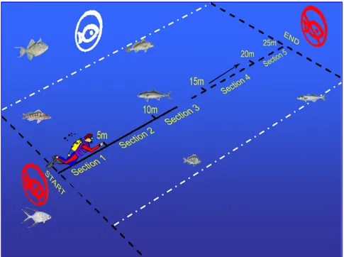
The observer conducts the 25 metres by 5 metres surveys by swimming along the central line of the transects following the reef profile. The observer counts all fish viewed within 2 metres on either side from the central line.

Figure 2.2: General scheme of visual census survey.

The reel layer follows the observer, laying the reel along the transect. The reel halyard is attached to a weight at the beginning of the transect.

During the scan of the section the most mobile target species are recorded, with progressively less mobile species recorded in subsequent counts. Fish entering the transect during, or after, the sampling of an area of transect are not included as they were not present during the initial count. Once the most

mobile species have been counted the observer moves along the central line of the transect searching for the more cryptic and slower moving target species, being careful to include also individuals of the most mobile species which were obscured from view by the structure of the reef during the initial count of the area.

2.2.2.a TIMING OF CENSUS

Sampling is not performed in high activity periods as arly morning and late afternoon to reduce variability in fish densities (due to diurnal influences on behaviour). Sampling has been limited to the hours between 09.00 and 16.30 during winter months and between 08.30 and 17.00 during summer months.

2.2.2.b DATA RECORDING

In addition to abundance estimates of target species, a number of ambient parameters are recorded which describe the physical environment at the time of census. Before entering the water numerous parameters related to weather conditions and location are recorded on the data sheets, i.e:

1. Code: the code name of the site.

2. Transect: the number of the transect, where transect 1 is the first transect of a site encountered.

3. Date: the date of census in the format DD/MM/YY.

4. Observer: initials of the observer carrying out the census.

5. Cloud: measured as the fraction of the sky covered by cloud and expressed in quarters, e.g. 0/4 indicates a cloudless sky, 3/4 indicates that approximately three quarters of the sky are obscured by clouds.

7. Sea: sea state:

□ Calm: mirror-like to small ripples □ Slight: large wavelets, crests breaking □ Moderate: many white caps forming □ Rough: large waves, 2-3m, white caps. 8. Sea: sea current

□ Absent: no current

□ Slight: no problems for divers

□ Moderate: diving is possible only in the current direction □ High: diving is not possible.

Once in the water, the following data are recorded prior to commencing the survey of each transect.

1. Depth: recorded to the nearest metre at the start of each transect. 2. Start: the time at which the census begins for each transect, recorded

in 24 hour notation e.g. 3.15 p.m. is recorded as 15.15.

3. Visibility: recorded when the observer first enters the water, prior to

census and expressed in metres distance. This is recorded only once,

unless it changes.

2.2.3 DATA MANAGEMENT

Due to the large volume of data collected during each survey trip, severe data management procedures must be followed to ensure safe and efficient storage of data.

The use of a laptop computer with data entry software is essential. On the same day of the data collection, observe the following procedure:

Rinse data sheets in fresh water and then dry them. Assign sample identification number to each transect.

Enter data onto laptop computer in the Access database (a user interface to Microsoft Access has been developed for this purpose).

Figure 2.3: The input mask.

Fish species names are entered in the database.

In office, data are checked and added to the main database using the following procedure:

□ Print raw data entered at sea and check against field data sheets. This checking procedure requires two personnel, one reads out the species and abundance data from the field sheets while the other checks these values against the print out of field entered data. □ Correct any error in the data and export to disk.

□ Give disk to database manager for inclusion into the Access database.

2.2.4 STATUS OF FISH STOCKS

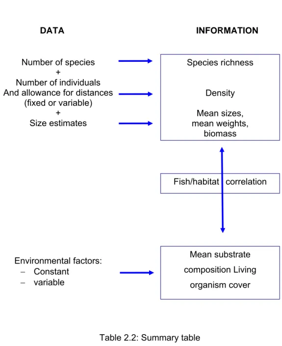
A) Identifying and counting species

Identifying and counting species provide an estimate of species richness (e.g. the number of species), particularly for environmental inventories. This can be limited to a sector of the population for food and/or commercial purposes or it can be conducted from an ecological point of view. This is an important parameter to consider. Any appreciable attack on the environment, such as the destruction of habitat, usually brings about a decrease in species richness, which is an indicator of biodiversity (e.g. number of species, and their percentage in the population).

B) Counting individuals

Individuals are counted to estimate abundance (number of fish) and density (number of fish per unit surface area) (e.g. individuals per square metre). Abundance and density are factors that can be affected by fishing activities and so, in certain cases, are a reflection of fishing intensity.

This method tends to bring about an underassessment of density and biomass (Labrosse P. et al. 2002). There is not a level of underassessment but it can be minimized with a regular training.

As with abundance and density, mean fish sizes and biomasses are parameters that are affected by fishing activities, particularly with regards to the most heavily targeted species. For example, in the specific case of untouched or unexploited stock, the introduction of fishing activities will rapidly lead to a decrease in mean size and biomass for the largest and most long-lived species.

Table 2.2: Summary table Environmental factors: − Constant − variable Fish/habitat correlation Species richness Density Mean sizes, mean weights, biomass Number of species + Number of individuals And allowance for distances

(fixed or variable) + Size estimates DATA INFORMATION Mean substrate composition Living organism cover

C) Statistical analysis

In order to gain an understanding of the community structure at and between sampling sites within the survey area, the following statistics indexes are applied to the data set for fish fauna.

LENGTH-WEIGHT RELATIONSHIP

Length-Weight relationships are important in fisheries science, notably to raise length-frequency samples to total catch, and to estimate biomass from underwater visual census length observations (Bohnsack J.A. and D.E. Harper, 1988).

LW is a mathematical formula for the weight of a fish in terms of its length; when only one of the two measures is known, the formula can be used to determine the other.

Typically given as:

b

L

a

W

=

∗

Where W is the weight, L the total length, a and b are coefficients referred to the studied fish (http://www.fishbase.org).

The units of length and weight are centimetres and grams, respectively.

ECOLOGICAL INDEXES AND DATA COVERAGE

To analyse community structure, spatial and temporal variability are tested analysing ecological indexes and data coverage.

Biodiversity

Biodiversity, or species diversity, is the simplest measure of species richness; it describes the variety and richness of life on the survey area. This index makes no use of relative abundances. It is expressed as: Biodiversity richness: S

Species Richness

The Margalef richness index adjusts the number of species sampled in a reference area by the logarithm of the total number of individuals sampled, summed over species. The higher the Margalef index, the richer the diversity of the population.

The formula is: Margalef richness: N S d ln 1 − =

Where S is the number of taxa and N is the number of individuals.

Shannon-Weaver index of diversity

The Shannon-Weaver index of diversity is simply the ecologist's definition of entropy expressed by:

Shannon-Weaver diversity:

∑

Where pi is the fraction of individuals belonging to the ith species. This is by

far the most widely used diversity index.

The minus sign is used to get a positive result, since probabilities are always less than one, and the logs of numbers less than one are always negative.

This measurement takes into account species richness and proportion of each species within the local aquatic community. This diversity index measures the order (or the disorder) observed within a particular system. In ecological studies, this order is characterized by the number of individuals observed for each species in the sample.

Pielou Evenness Index

This evenness index, is a measure of how evenly distributed abundance is among the species that exist in a community. The Pielou index is defined between 0 and 1, where 1 represents a community with perfect evenness, and the index decreases to zero as the relative abundances of the species diverge from evenness. The Pielou index is calculated for each sample as:

Pielou index: S H J log =

Where H is the Shannon-Wiener Index for the sample and S is the number of taxa.

Bray - Curtis index

The Bray-Curtis index measures the degree of difference in community structure (especially community composition) between sites. This measure helps to evaluate the amount of dissimilarity between benthic invertebrate communities at different sites.

Bray - Curtis index

(

)

n

n

n

n

BC

Simpson's Index of Diversity 1 - D

The index is a measure of the character of a community that takes into account both the abundance patterns and the taxonomic richness of the benthic invertebrate community. It is calculated from the proportion of individuals which belongs to each taxonomic group contribuiting to the total sample.

The value of this index ranges between 0 and 1, the greater the value, the greater the sample diversity. In this case, the index represents the probability that two individuals randomly selected from a sample will belong to different species.

Analysis of differences

Analysis of differences in fish assemblage structure was conducted using multivariate non-Metric Multidimensional Scaling ordination (MDS) and Bray-Curtis cluster analysis using the computer package PRIMER (Clarke K. R. and Warwick R. M., 1994). The Bray-Curtis similarity index was applied on square-root transformed data (to down-weight the influence of rare and extremely abundant species) generating a rank similarity matrix, which was then converted into an MDS ordination (Clarke K. R., 1993). To check on the adequacy of the low-dimensional approximations seen in cluster and MDS, the use of PRIMER v6.1.5 enabled clusters to be superimposed upon the MDS ordination (Clarke K. R. and Gorley R. N., 2006). One/two-way ANOSIM was used to investigate differences identified from MDS and cluster (Clarke K. R. and Warwick R. M., 1994). SIMPER analysis was used to ascertain the fish species that contributed most to the dissimilarity between sites and time.

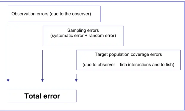
2.2.5 SOURCES OF ERROR

No assessment method is perfect and Underwater Fish Visual censuses also include sources of error. Errors mainly come from one of this three sources: the observer, the fish behaviour, and the sampling method. Understanding these sources of error is vital for both minimising them, and taking them into account during analysis and interpretation of the results.

Table 2.3: Sources of error.

Sources of error due to the diver

Due to diving time restrictions and to the often shy nature of the animals surveyed, observers must be able to record informations as quickly as possible, and to rapidly identify and estimate sizes and distances with a reasonable level of accuracy. The slightest hesitation will result in a loss of data. Observers may pay more attention to one group of fish or to a part of the population that interests them more: this is a systematic error. Observers may also have a tendency to overestimate or underestimate sizes and/or

Observation errors (due to the observer)

Target population coverage errors (due to observer – fish interactions and to fish) Sampling errors

(systematic error + random error)

distances. Moreover, there is always the risk of counting the same fish several times. Finally, for counts at variable distances, consideration must be given to the fact that fish detection ability tends to increase with size for almost all species, and with the size of the school for certain fish (number of individuals in a school).

Hesitation, inattention or paying too much attention to a certain area, are all increased when the conditions under which the census is being conducted worsen (e.g. strong currents, fatigue or cold) or when the quantity of information to be recorded is too great (too many species, too many fish). As a result, environmental, psychological, and physical conditions of observers’ work should have as little influence as possible. This means that observers should master diving techniques and not to be subject to disturbances that reduce the acuity of their eyesight and/or their motor skills.

Sources of error due to observer–fish interaction

Such interactions mainly involve changes in fish behaviour due to the diver’s presence. These changes vary and may result in either the fish fleeing away from, or being attracted to, the diver. For example, some species, such as those from the Serranidae genus, tend to be attracted to observers and follow them around. In contrast, Sparus aurata tends to keep away by remaining at the limit of visibility. Such behaviour also depends on the individuals’ activity cycle (diurnal vs. nocturnal), age and location. The simultaneous trajectories of fish and observer can bring about either negative or positive biases in size estimation, depending on whether they are swimming in the same direction or

in opposite directions with a visual angle that differs more than 90° from the transect.

The diver’s movement as well as the method used, also has an influence on fish behaviour (e.g. the noise from air bubbles coming out of scuba diving equipment).

Regular visits to a site, particularly for monitoring, tend to decrease attraction or fleeing reactions, thus minimising these biases.

Sources of error due to fish

The main sources of error due to fish come from the distribution of species in time and space. This depends on different parameters associated with habitat, behaviour and activity cycles.

Certain species, which are sedentary during the day and that come out only at night, may not be detected by observers. Similarly those fish that come out of their hiding places only briefly, those that are highly mobile, or those which colonise certain biotopes during certain seasons can be missed. The probability of encountering species and thus being able to count them is influenced by their behaviour and their home range or territory. This is why it is difficult to make a comprehensive assessment of fish populations. It should also be noted that populations seen and sampled only account for a portion of all the species that live in the study area.

The various biological and ecological characteristics of fish influence measurements and estimates. Any interpretation of results must take into account that not all species are perceived (and therefore estimated) in the same way.

Sources of error due to sampling

Most sampling errors arise because results depend not only on the elements (all transects or stationary points) that make up the sample, but also on the method itself.

A sample is a limited subset of a population, from which the results obtained from the observed data are based. For technical, economic or simply logistical reasons (destruction of specimens, as when fish are caught by experimental fishing), it is normally not possible to collect data on the entire population. The study of a limited set makes it possible to increase both the number of measurements and their degree of accuracy.

Extrapolation of the findings obtained from sampling generally results in estimates for the entire population, which have a reasonable level of accuracy. If two samples composed of a given number of elements (set of transects or stationary points) are observed, the measurements calculated for each will be different, but they will result in comparable estimates of population parameters. The statistical population is defined as a set of entities on which statistical inferences and conclusions are based. Samples not taken according to a strict sampling plan (random or reasoned) will not be representative of the target fish population. The sample is considered to be equal to the statistical population.

The position of a transect and orientation can be considered sources of error associated with sampling. It is preferable a transect that covers an homogeneous environment, rather than one covering several different environments. Transitional areas between different biotopes should be

The accuracy of population estimates depends on the size of the sample (number of transects) and variability (differences between the measurements for each transect). This variability in individual measurements or random error (dispersion) must not be mistaken for systematic error (bias).

Four model situations are given:

Lack of accuracy can be linked to high bias and/or high dispersion.

Sampling-related bias can be reduced through a random selection of sample elements.

Errors in observation and representativity do not decrease when the size of the sample increases.

Dispersion depends on the population’s heterogeneity. It is measured by variance.

When dispersion is high (i.e. there are significant differences between transects), better estimates will be gained by stratifying the population (e.g. by biotope).

How to limit sources of error

Firstly, new observers are trained, in situ, in the identification of the target species, and in the standard technique for visual census of belt transects. Secondly, experienced observers are continually standardised to minimise inter-observer bias.

Moreover, new observers and experienced observers must keep in mind that divers should have regular training to minimise errors caused by poor diving techniques.

The fish identification is the first step of training. The first key to identify fish is their shape, which is generally the same for almost all the species in a given

family. The visual morphological characteristics that identify a species within a family are shape, colour of markings, and distinctive traits such as spots, lines or stripes, and their location on the body and/or fins. Behaviour and preferred biotopes are also useful for identification. Learning and retention of these features are necessary, though they are perhaps the most tedious part of training. The appearance of some fish changes over the life cycle; for example, many Perciformes like Coris julis, have different colours during their juvenile and adult phases and colours can differ according to sex.

Training in fish identification involves classroom - learning using available tools, and onsite exercises during dives. In order to avoid confusion over the use of common names, it is preferable to use each species’ scientific name, which is always made up of a genus name (e. g. Coris, the genus) followed by a species name (e. g. julis); thus forming the name Coris julis).

A list of fish , which are of food and commercial interest, is given in.

If fish from a certain family cannot be precisely identified during a dive, the observer must rapidly note its main features (e. g. shape, colours, and markings) so as to be able to complete the identification through books afterwards. The use of simple sketches to illustrate and record specific marks on the body is invaluable.

Identification skills are further enhanced with underwater coaching where an experienced observer points out target species and highlights physical characteristics, habitat preferences and behavioural patterns that will aid in quick and accurate identification.

Moreover, precise counting cannot be carried out on more than 10 to 20 individuals in a relatively sedentary school. Taking into account these limits, and in order to compensate for them, the most commonly used technique for counting schools is the so-called group-counting method. This consists of counting a shoal of 10 to 20 fish. This group becomes the basic counting unit and the observer judges how many groups there are in the entire area occupied by the school of fish. For large schools (more than 200 individuals), it may be useful to combine groups into super-groups, containing 5 to 10 base groups.

In more complex instances where a shoal of fish is made up of several different species (multispecies shoal), observers begin with the count of the most numerous species. The same applies to shoal with a range of sizes. During training, taking photographs is a good way to evaluate errors made, and to find out at what level they occurred.

Observers undertake annual standardisation exercises to maintain significantly close concordance in their counts. The procedure used for inter-observer standardisation is identical to that outlined above for the training of observers in the visual census technique.

2.3 SAMPLING DESIGN

Sampling sites were chosen in the pre-survey after eight months of diving (first eight months of the 2004).

Sampling time were scheduled as follows: Time 1: September – November 2004; Time 2: June – July 2005; Time 3: September – November 2005; Time 4: June – July 2005.

Six sectors of the reef fish communities were surveyed every six months (in autumn and spring) within and around the MPA (Cala Pira, Isola di Serpentara, Capo Carbonara, Isola dei Cavoli, Solanas and Torre delle Stelle sectors). The sampling sites are the places where the surrounding area was best represented (the analyzed site had the ecosystemic characteristic of the entire area).

Habitat was surveyed on each reef. It is described as the first stretch of continuous reef with a slope less than vertical. Similar habitats were selected to allow comparisons between sectors.

Transects were set within the sectors, along the middle of the reef slope (usually at a depth between two and eight metres). A total of eight replications in every transect were made. Each replication was 25 metres long and four metres wide (two per each side).

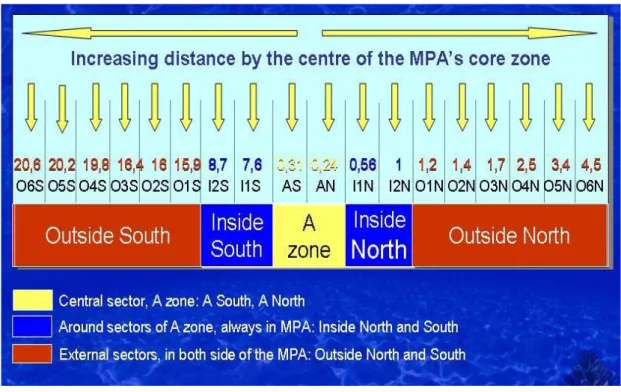
Figure 2.5: Fish visual census, distances by the center of the core zone.

The sampling sites are shown in figure 2.4: Yellow tags represent the sites in the central sectors, the core zone (A zone); Blue tags the sites inside the MPA (in B or C zones); Red tags the sites located out of the MPA border. Transects are at increasing distance from the core zone.

The exact latitude and longitude of the sampling sites are reported in table 2.3.

To study fish fauna with visual census technique, a set of 24 targets species has been selected. All of them are usually object of fishing activities inside and outside the MPA.

ACRONYM POSITION ACRONYM POSITION

A1N N39 09.138 E9 36.171 O2S N39 07.321 E9 26.269 A1S N39 08.147 E9 36.187 O3N N39 10.011 E9 34.236 I1N N39 08.182 E9 36.373 O3S N39 07.501 E9 26.087 I1S N39 05.052 E9 32.361 O4N N39 10.586 E9 34.776 I2N N39 08.823 E9 33.997 O4S N39 08.606 E9 24.188 I2S N39 05.908 E9 31.004 O5N N39 11.025 E9 34.692 O1N N39 09.363 E9 34.051 O5S N39 08.498 E9 24.107 O1S N39 07.399 E9 26.392 O6N N39 11.269 E9 34.101 O2N N39 09.697 E9 34.131 O6S N39 08.534 E9 23.906

Grid Lat/Lon ddd°mm.mmm'; Datum: WGS 84

Table 2.3: Latitude and longitude of the sampling sites.

TARGET SPECIES

Coris julis Labrus merula Scorpaena porcus

Dentex dentex Labrus viridis Scorpaena scrofa

Dicentrarchus labrax Lithognathus mormyrus Serranus cabrilla

Diplodus puntazzo Mullus surmuletus Serranus scriba

Diplodus sargus Pagrus pagrus Sparus aurata

Diploids vulgaris Sarpa salpa Sphyraena sphyraena

Epinephelus costae Sciaena umbra Symphodus tinca

In four Times of sampling, a total of 432 replications were performed: 144 inside the MPA (48 in the A zone and 96 inside the sanctuary), and 288 outside.

Figure 2.5: Example of recorded data.

A total of 6156 records were carried out and distinguished by species, size, amount and unequivocal sampling code.

2.4 RESULTS AND DISCUSSION

Preliminary snorkel and SCUBA surveys were used to create a list of target key species (in particular commercially important species) of fish found within all of the study sites.

The list of the 24 target species subdivided by taxonomic rank is scheduled in the appendix 5.

The 24 target species are listed by presence in the three sampling Zones.

TARGET SPECIES A ZONE INSIDE OUTSIDE

Coris julis

+ + +

+ +

+

+ + +

+ + +

+ + +

+ + +

+ +

+ +

+ + +

+ + +

+ +

+ +

+ + +

+ +

+

+ + +

+ + +

+ +

+ +

+ + +

+ + +

+ + +

In three years of sampling, a total of 8550 specimen were observed in the studied area.

Mean weight

The output of elaborated data from Length-weight relationships used for the studied target species was processed to obtain the mean weight of biomass for Sites in A zone (A) of the MPA, Inside the MPA (I) and Outside (O). These results showed high values of biomass in the inside zone in autumn season.

Graph 2.1: Total mean weight from the Core Zone (A, North and South), Inside Zone (I, North and South) to Outside of the boundaries (O, North and South); all weight are listed by Time of sampling (Time 1-2-3).

It is due to the fry. During this season, mean fish biomass was high in A Zone and spillover effect resulted from A Zone (Time 1) to Outside in the southern sampled sites in Time 2; what was more, a general increase in all the studied sites was observed from Time 1 to Time 3 indicating the effectiveness of the established MPA.

Mean weight of all the samplings scheduled by specimen are listed in appendix 6. 0 1 2 3 4 5 6 7 8 6 5 4 3 2 1 2 1 1 1 1 2 1 2 3 4 5 6 6 5 4 3 2 1 2 1 1 1 1 2 1 2 3 4 5 6 6 5 4 3 2 1 2 1 1 1 1 2 1 2 3 4 5 6 O I A A I O O I A A I O O I A A I O S N S N S N

Time 1 Time 2 Time 3

T o tal w e ig h t (m ean )