UNIVERSITÀ DEGLI STUDI DI CATANIA
FACOLTÀ DI INGEGNERIA
Dottorato di Ricerca in Ingegneria Elettronica, Automatica e del Controllo dei Sistemi Complessi
XXIV CICLO
Tesi di Dottorato
AGNESE DI STEFANONext generation of numerical models for inferring the volcano dynamics from geophysical observations
Tutors: Prof. Eng. Luigi Fortuna Dr. Ciro Del Negro Eng. Gilda Currenti Coordinator: Prof. Eng. Luigi Fortuna
Acknowledgements
A sincere thank goes to my tutor and Ph.D. school coordinator Prof. Eng. Luigi Fortuna who, first, gave me the possibility to have this experience and always represented a reference point in my scientific path.
I would like to express my gratitude to my tutor Dr. Ciro Del Negro for supervising my work and for offering his expertise to make me develop my knowledge about Volcano Geophysics.
I am grateful to the members of the the research groups of the the “Unità Funzionale Gravimetria e Magnetismo” at “Istituto Nazionale di Geofisica e Vulcanologia” for their support and patience. Especially I’d like to thank Eng. Gilda Currenti for her professional and personal support; she represented a strong stimulus and inspiration in my research activity.
Last but not least, I deeply thank my family, to be always ready to support and encourage me even in the difficulties, giving me the certainty that I would never have been alone.
Index
Introduction ... 1
Chapter 1 Numerical Methods: FE Modeling of Ground Deformation, Piezomagnetic and Gravity Fields ... 11
1.1 Governing equations of ground deformation, piezomagnetism and gravity ... 13
1.2 Numerical model ... 20
1.3 Comparison Between Analytical and Numerical Results ... 23
1.3.1 Piezomagnetic and gravity field generated by pressure source .. ………24
1.3.2 Piezomagnetic and gravity field generated by intrusive source ... 30
1.4 Discussions ... 33
Chapter 2 Effects of Heterogeneity and Topography on Piezomagnetic Field... 35
2.1 Heterogeneity effect ... 37
2.1.1 Effects of elastic heterogeneity……..………37
2.1.2 Effects of magnetic heterogeneity………..41
2.2 Topography effect ... 47
2.3 Discussions ... 50
Chapter 3 Application to Real Case Studies at Etna Volcano ... 53
3.4 Discussions ... 85
Chapter 4 FEM and ANN combined approach for predicting pressure sources at Etna volcano ... 91
4.1 Forward Problem: FEM solution ... 93
4.2 Neural Network model ... 100
4.3 Identification results ... 103
4.3.1 ANN based inverse model……….……103
4.3.2 ANN based forward model………...…....111
4.4 Discussions ... 114
Conclusions ... 116
List of tables
1.1 Pressure source geometry and medium properties. 25 1.2 Intrusive source geometry and medium properties. 31 2.1 Model properties. The magnetic structures JA and JB
are described in Fig. 2.3.
37 3.1 Source geometry and medium properties by Bonforte
et al. (2008). 62
3.2 Gravity variations related to 2005-2006 period observed at the monitoring stations at Mt. Etna after
having been corrected for free air effect. 68 3.3 Chi-square values of deformation and magnetic
changes for the analytical and the numerical models. 80 4.1 Ranges of the random generated parameters of the
source. 97
4.2 Performance indexes RMSE and E%abs for the
inversion of analytical and numerical deformation
model and for the integrated numerical model. 105 4.3 Performance indexes RMSE and normalized misfits
δm for two stations located near (A in Fig. 4.4) and
List of Figures
1.1 Computational domain and boundary conditions for the deformation.
21 1.2 Computational domain for magnetic and gravity
problem.
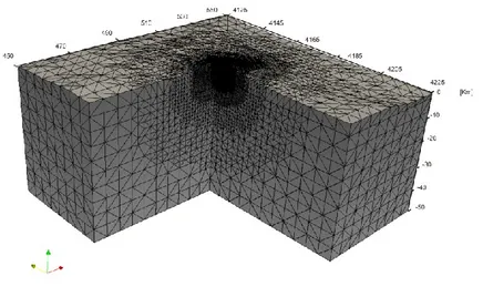
22 1.3 Meshed domain of the numerical model. The mesh is
refined around the volcano structures and becomes coarser at greater distance..
23
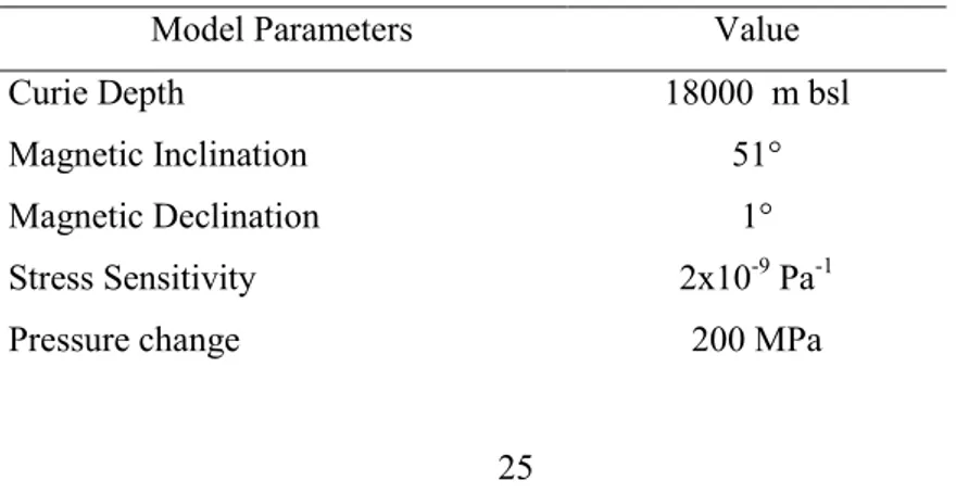
1.4 Comparison between the analytical solutions (color scale) and the numerical results (line). Contour lines are at 0.5 nT intervals. Profiles along NS and EW directions are reported for the analytical (line) and numerical (circles) models.
28
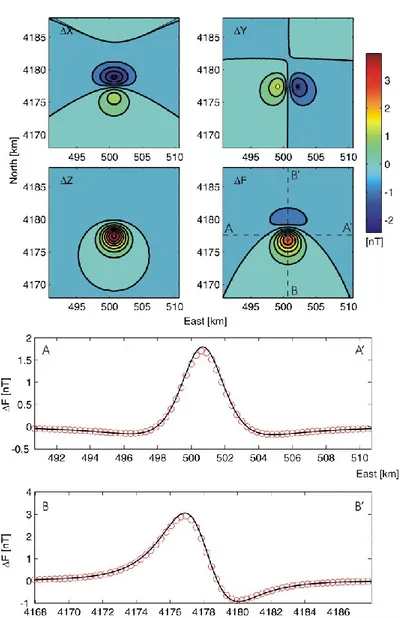
1.5 Comparison between the analytical solutions (color scale) and the numerical results (line) of gravity field.
29 1.6 Displacement at the source wall along a section at
z=-800 m in a 3D view. Red and blue colors represent the positive and negative displacement along the x-axis respectively.
32
1.7 Comparison between the analytical solutions (color scale) and the numerical results (line) of piezomagnetic variation generated by a dyke source. Contour lines are at 10 nT intervals.
32
1.8 Comparison between the analytical solutions (color scale) and the numerical results (line) of gravity variation generated by a dyke source. Contour lines are at 5uGal intervals.
2.1 Young modulus distribution (a) and Poisson ratio distribution (b).
38 2.2 Total intensity of piezomagnetic field produced by a
pressure change (a) and a volume change (b) in a spherical source for the half-space model B, which is homogeneous in magnetic properties and heterogeneous in elastic parameters. Contour lines are at 0.5 nT intervals. The star represents the pressure source location.
39
2.3 Layered structures of the initial magnetization free from stresses. On the left the JA two-layered magnetization structure, on the right the JB three-layered magnetization structure.
42
2.4 Geological based model of Mt Etna by Tibaldi and Groppelli.
44 2.5 The total piezomagnetic field for the half-space
models C (a) and D (b). Contour lines are at 0.5 nT intervals.
45
2.6 Total intensity of piezomagnetic field (contour lines at 0.5 nT intervals) for the half-space models E (a) and F (b).
46
2.7 Mesh of the topography of Mt Etna. 47
2.8 The magnetic field changes for a homogeneous magneto-elastic medium with the real topography of Mt Etna. Contour lines are at 0.5 nT.
48
2.9 Total intensity of piezomagnetic field for the models E (a) and F (b) with the real topography of Mt Etna. Contour lines are at 0.5 nT intervals.
49
3.1 Continuous GPS monitoring network at Mt Etna. 54 3.2 Gravity and magnetic monitoring networks at Mt
Etna
54 3.3 Distribution of Young Modulus (a) and rock
magnetization (b) in numerical model of Mt Etna.
3.5 Gravity anomaly observed at Mt Etna during the period 2005-2006. Contour lines are at 10 Gal.
60 3.6 Source modeled by Bonforte et al. (2008) represented
by an ellipsoidal pressure source and a sliding plane, together with the comparison between the observed and the modelled ground deformation vectors.
61
3.7 Section of the mesh of the computational domain. 63 3.8 Comparison between deformation field observed at
the GPS stations at Mt. Etna (blue arrows) and computed deformation field generated by the pressure source (green arrows). Contour lines (at 1 cm intervals) represent the vertical displacement anomaly computed with the numerical model.
64
3.9 Piezomagnetic anomaly (contour lines at 0.1nT) generated by the pressure source. The black circles are the magnetic stations of monitoring network at Mt. Etna.
65
3.10 Thermomagnetic anomaly (contour lines at 1nT) generated by the pressure source. The black circles are the magnetic stations of monitoring network at Mt. Etna. Inset shows the magnetic variations observed at the monitoring stations.
66
3.11 Gravity anomaly (contour lines at 2.5μGal) generated by the pressure source. The black circles are the gravity stations of monitoring network at Mt. Etna.
67
3.12 Schematic map of the Etna summit area covered by the lava flows of the 2008 eruption. Locations of magnetic, gravity and GPS stations are also shown. Inset shows the position of the CSR magnetic
3.13 Magnetic observation at the magnetic stations during the 2008 eruption at Mt Etna.
71 3.14 (A) Radial (rad) and tangengential (tan) tilt
components recorded during the 713 May 2008 intrusion. (B) Selected North–South (N–S) and East–West (E–W) position components recorded by the GPS network. The signals are smoothed using a mobile average with a 10-min duration window. The grey box indicates the first phase of the intrusion (Aloisi et al, 2009).
72
3.15 View of the mesh of computational domain, with a high resolution in the areas near the source.
74 3.16 Comparison between analytical solutions (a) and
numerical results of model A (b) for the 2008 intrusive source from Napoli et al. [2008]. Piezomagnetic change (contour lines at 2 nT) generated by the intrusive dike (black line). Observed (blue arrows) and computed (red arrows) deformation at the permanent GPS stations are also reported. The recorded magnetic changes are reported in the inset.
75
3.17 Comparison between measured and computed magnetic changes for the analytical and numerical models..
76
3.18 Gravity contributions generated by the intrusive source using the analytical solution. Contour intervals are 1 µGal for g1 (a), 10 µGal for g2 (b), 2 µGal for g3 (c) and 10 µGal for the total gravity change (d). Black circles represent the gravity stations of the monitoring network at Mt. Etna.
intervals are 1 µGal for g1 (a), 10 µGal for g2 (b), 2 µGal for g3 (c) and 10 µGal for the total gravity change (d). Black circles represent the stations of the gravity monitoring network at Mt. Etna.
3.20 Piezomagnetic changes, ground deformation (a), and gravity changes (b) caused by the magmatic intrusion in model B. Observed (blue arrows) and computed (red arrows) deformation at the permanent GPS stations are also reported. Contour intervals are 2 nT for the piezomagnetic changes (a) and 10 µGal for gravity changes (b).
81
3.21 Normal displacement to the dike wall in the numerical model D. The dilation profile (opening exaggerated by a factor 300) for an overpressure of 13 MPa is also reported (black line).
84
4.1 Mesh of the computational domain. The mesh has a spatial resolution of 300 m in the summit area and around the source location and becomes coarser at greater distance.
97
4.2 Parallelization of procedure on a cluster of 20 nodes. 99 4.3 Deformation pattern of the vertical component. 99 4.4 Permanent GPS (red circles), gravity (yellow squares)
and magnetic (blue triangles) stations of the monitoring networks on Mt Etna. The black rectangle corresponds to the projection on surface of the volume where the sources are located.
100
4.5 Block diagrams of inverse (a) and forward (b) model identification.
102 4.6 Structure of Artificial Neural Network for inversion
of geophysical models.
4.7 Predicted values of source parameters with respect to output patterns of the testing set for the integrated numerical inversion.
108
4.8 Mean percent error E%abs for each source parameter
using noisy deformation patterns at the inputs of the ANN inverse model.
110
4.9 Mean percent error E%abs for each source parameter
using noisy patterns at the inputs of the integrated ANN inverse model.
Introduction
Eruptions are the culmination of long-term evolution in the volcano plumbing system. The complexity of volcanic systems originates from the large variety of physical processes which may precede and accompany the ascent of magma to the Earth’s surface and its eruption. During ascent magma interacts with surrounding rocks and fluids and almost inevitably geophysical signal variations are produced.
Monitoring involves geophysical, seismological or geochemical techniques that detect magma movements and associated sub-surface interactions, through physical measurements, which are made both at the earth’s surface and within the earth’s subsurface.
Over the last decades, new modern techniques of volcano monitoring have been implemented on active volcanoes in order to improve the knowledge of eruptive processes. The characterization of geophysical signals can be a useful tool both for improving the monitoring of
pre-eruptive mechanisms which produce them.
However, field data alone are not enough for making any quantitative interpretation, but in addition model responses are needed. By examining together field data and model data, the quantitative statement of the structure and dynamics of the volcanoes can be examined. Mathematical models have become key tools, not only to forecast the dynamic of the volcanic activity, but also to interpret a wide variety of geophysical observations, which have provided further insights into the complex dynamics of eruptive processes.
Magma migration inside a volcano edifice generates a wide variety of geophysical signals, which can be observed before and during eruptive processes. In particular, ground deformation, gravity and magnetic changes in volcanic areas are generally recognized as reliable indicators of unrest, resulting from the intrusion of fresh magma within the shallow rock layers. If the volcanic edifice can be assumed to be elastic, contributions to geophysical signal variations depend on surface and subsurface mass redistribution driven by dilation/contraction of the volcanic source. Indeed ground deformation studies provide insight about volume changes in the magma reservoir and the dynamics of dike intrusion processes (Voight et al.1998; Battaglia et al., 2003 Murase et al. 2006). However, deformation data alone are not able to properly constrain the mass of the intrusions. Geodetic studies need to be supported also by gravity observations in order to infer the density of the intrusive body and better define the
changes are strictly related each other. Indeed, changes in the gravity field cannot be interpreted only in terms of gain of mass disregarding the ground deformation of the rocks surrounding the source. Contributions to gravity changes depend also on surface and subsurface mass redistribution driven by dilation of the volcanic source. Moreover, in volcanic areas, significant correlations were observed between volcanic activity and changes in the local magnetic field, up to ten nanoteslas (Del Negro and Currenti, 2003). These observations were compared with those calculated from volcanomagnetic models, in which the magnetic changes are generated by stress redistribution due to magmatic intrusions at different depth and by the thermal demagnetization at a rather shallow depth. The magnetic data not only allowed the timing of the intrusive event to be described in greater detail but also, together with other volcanological and geophysical evidences, permitted some constraints to be set on the characteristics of propagation of shallow dikes (Del Negro et al., 2004).
The comparison between these observations and geophysical models allowed inferences about volcanic source parameters and detailed descriptions of magma migration, but limited efforts have been made for effective integration of these different data. These geophysical signals are generally interpreted separately from each other and the consistency of interpretations from these different methods is qualitatively checked only a posteriori. Anyway, when the cause of these geophysical signal variations can be ascribed to the same volcanic source, an integrated approach based on different
for inferring magmatic intrusions and minimizing interpretation ambiguities (Nunnari et al, 2001; Currenti et al., 2011).
Ground deformation, gravity and magnetic variations due to volcanic sources have been modeled separately using analytical solutions, based on simple homogeneous elastic half-space models (Bonaccorso and Davis, 2004; Carbone et al 2007; Del Negro and Currenti, 2003; Del Negro et al 2004; Napoli et al, 2011). Analytical elastic models are attractive because of their straightforward formulation. The drawbacks of the analytical formulations for modeling volcanic activities are the assumption of simple geometries for the sources embedded in homogeneous elastic half-space. Nevertheless natural characteristics of volcanic areas such as topography or lateral variations of rheological properties may have great influence on the observed signals: such complexities can be treated using numerical methods. The most adequate method to calculate stress and strain and hence deriving associated geophysical signals changes in a given material is the finite element method (FEM). This method allows to overcome these intrinsic limitations and provide more realistic models, which allow considering topographic effects as well as heterogeneous distribution of medium properties.
We dealt with the problem of the interpretation of geophysical data in order to analyze quantitatively the structure and dynamics of volcanoes. Improving forward models with FEM is the starting point for the geophysical processes representation, but the inverse modeling,
significant changes in geophysical observations recorded by monitoring networks, is the principal goal of modeling in geophysics. Inverse problems are usually formulated and solved as optimization problems based on iterative procedures, minimizing an objective function that quantifies the misfit between the observed data and the estimated solutions from forward models. Analytical solutions are often used to represent the forward model because of computational convenience and fast computer implementation (Currenti et al., 2005; Nunnari et al., 2005). Numerical solutions allow to overcome the intrinsic limitations of analytical models, but the use of numerical forward models in iterative methods is computationally expensive since the estimate of the objective function requires to perform a full FEM analysis at every iteration step. As traditional optimization algorithms cannot “learn”, they cannot benefit from solutions obtained previously for similar problems and each new inversion requires the minimization procedure to be re-iterated.
Recently, Artificial Neural Networks (ANNs) have been introduced to solve the inverse problem in many research applications (Haykin, 1999, Arena et al., 1998). The main advantage of inverting with ANNs consists in the availability of an approximation of the inverse model, avoiding a search for the minimum and speeding up the computation of the optimal solution that fits the observed data. ANNs have been widely used to invert geophysical models based on straightforward analytical solutions (Langer et al., 1996; Maugeri et al., 1996; 1997; Nunnari et al. 2001) because of low computational effort. On the contrary, FEM-based numerical solutions are not often
both in length of time required to design a mesh and in actual computation time. With the advent of today’s powerful computer resources and the automation of mesh generation and FEM analysis, hybrid schemes based on FEM and ANN have been proposed in different applications (Hacib et al., 2007; Preda et al, 2002; Ziemianski, 2003; Ajmera et al., 2008; Szidarovszky et al., 1997; Chamekh et al, 2009; Muliana et al., 2002; Saltan et al., 2007; Umbrello et al., 2008).A promising method to address the issue of geophysical modeling should be a hybrid approach using FEM and ANN to model jointly geophysical signals as deformation, gravity and magnetic signals (Di Stefano et al, 2010). We investigate the ability of a hybrid procedure in which ANNs are used for system identification of forward and inverse geophysical models solved by FEM.
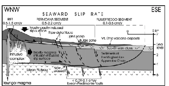
The discussed approaches for interpretation of geophysical data are successfully applied to Etna volcano, which offer exemplary case studies to validate the capability of the proposed integrated approach for imaging the pressurization and intrusive processes occurring in the volcano. Volcanological tradition is consolidated at Mt Etna and advanced monitoring networks enabled collecting multi-disciplinary data during the frequent eruptions in recent years (Rymer et al, 1998). Geodetic, gravity and magnetic investigations have played an increasingly important role in studying the eruptive processes at Mt Etna (Napoli et al., 2008; Bonforte et al., 2008; Carbone et al., 2007; Del Negro et al., 2004; Bonaccorso et al, 2011). Moreover, as
et al., 2000; Tibaldi and Groppelli, 2002), the Etna volcano is elastically inhomogeneous and rigidity layering and heterogeneities are likely to affect the magnitude and pattern of observed signals (Currenti et al., 2007; 2009). So the volcano complex structure can be well represented by the proposed numerical models.
The aim of this thesis is, starting from the simplified analytical geophysical models to reach the more realistic integrated numerical model for ground deformation, magnetic and gravity field variations generated from a volcanic source. Indeed the FEM should provide a more precise description including realistic features for the source shape, the topographic relief, the elastic medium heterogeneities and the density stratifications.
In Chapter 1 a joint forward formulation of deformation, piezomagnetic and gravity data is provided through a FEM coupled model, in order to overcome the limitation proper of the analytical forward in terms of half-space and at the same time don’t mistreat the multi-parametric approach. All the geophysical changes were evaluated by solving an elastic homogeneous problem both for pressure source and intrusive sources, in order to compare analytical and numerical solution. 3-D elastic models based on finite element method (FEM) have been developed to compute piezomagnetic and gravity fields caused by magmatic overpressure and dyke sources. We solved separately (i) the elastostatic equation for the stress field and (ii) the coupled Poisson’s equation for magnetic and gravity potential field.
heterogeneities and topography were evaluated in Chapter 2. The numerical computations were focused on a more realistic modelling of Etna volcano, where remarkable geophysical changes have been observed during eruptive events. The effects of topography and medium heterogeneities were evaluated considering different multilayered crustal structures constrained by seismic tomography and geological evidences.
The FEM approach presented here allows considering a picture of a fully 3-D model of Etna volcano, which could advance the reliability of model-based assessments of magnetic observations.
In Chapter 3 successively a 3D finite element modeling was set up to analyze two case studies: the first was the 2005-2006 inflation period at Mt Etna, the second one was the magmatic intrusion occurring in the northern flank of Etna during the onset of the 2008 eruption. A 3D numerical model based on Finite Element Method (FEM) is implemented to jointly evaluate geophysical changes caused by dislocation and overpressure sources in volcanic areas. A coupled numerical problem was solved to estimate ground deformation, gravity and magnetic changes produced by stress redistribution accompanying magma migration within the volcano edifice.
A multi-layered crustal structure of the volcano constrained by geological models and geophysical data was considered. Geodetic and gravity data provide information on the strain field, while piezomagnetic changes give constraints on the stress field. Therefore,
overpressure involved in the magma propagation and improves understanding of dike emplacement in the northern sector of the volcano.
The last challenging scope of this thesis, described in Chapter 4, was to solve a numerical integrated inverse problem. A hybrid approach for forward and inverse geophysical modeling, based on Artificial Neural Networks (ANN) and Finite Element Method (FEM), is proposed in order to properly identify the parameters of volcanic pressure sources from geophysical observations at ground surface. The neural network is trained and tested with a set of patterns obtained by the solutions of numerical models based on FEM. The geophysical changes caused by magmatic pressure sources were computed developing a 3-D FEM model with the aim to include the effects of topography and medium heterogeneities at Etna volcano. ANNs are used to interpolate the complex non linear relation between geophysical observations and source parameters both for forward and inverse modeling. The results show that the combination of neural networks and FEM is a powerful tool for a straightforward and accurate estimation of source parameters in volcanic regions.
Chapter 1
Numerical Methods: FE
Modeling of Ground
Deformation, Piezomagnetic
and Gravity Fields
Before eruption, magma chamber pressurization and magma ascent to the Earth’s surface force surrounding crustal rocks apart and this perturbs stress distributions, commonly producing variations in the magnetization and density of rocks, resulting in a local magnetic field and gravity field change (Nagata 1970; Pozzi 1977). Gravity and
piezomagnetic changes are calculated by combining the Cauchy– Navier equation for elastic equilibrium and the Poisson’s equation for the magnetic and gravity potential (Sasai 1986; Utsugi et al. 2000). The analytical solutions are derived by employing important simplifications and approximations (Sasai, 1991a; 1991b; Utsugi et al., 2000). Most of the analytical formulations are based on the assumption of a volcanic source embedded in a homogeneous magneto-elastic half-space medium (Sasai, 1991b). Analytical elastic models are attractive because of their straightforward formulation. However, volcanic areas are usually characterized by severe heterogeneities and irregular topography that are responsible for significant effects. Although numerical procedures have been applied in ground deformation studies to estimate how topography and heterogeneity can affect the deformation field solution (Williams and Wadge 1998; Williams and Wadge 2000; Cayol and Cornet 1998; Lungarini et al. 2005; Trasatti et al, 2008; Bonaccorso et al., 2005; Currenti et al., 2008), few studies have been performed on the piezomagnetic and gravity field. We developed a coupled numerical model using the Finite Element Method to compute jointly the deformation, gravity and magnetic changes caused by dislocation and pressure sources. The FEM is suitable to easily solve the model equations and to account for topography and medium heterogeneity, which can alter the estimate of the investigated geophysical changes. Comparisons are made between analytical and numerical solutions
sources and dislocation sources embedded in a homogeneous half-space elastic medium, with the aim to properly set up the model and verify the accuracy of the numerical solution.
1.1 Governing
equations
of
ground
deformation, piezomagnetism and gravity
In order to find the state of stress and displacement that results from the application of certain loads or boundary displacement, it is necessary to solve a set of three coupled partial differential equations known as “equations of stress equilibrium”. These equations are found by using the Newton’s second law and can be expressed in the following vector/matrix form:
2 2
t
σ
F
u
(1.1)Where F is the body force, is the stress tensor and is the density of the material.
The equations of motion, along with the strain-displacement relations and the stress-strain relations, constitute a set of equations in which the number of unknowns is equal to the number of equations. In the frequently occurring case in which the rock is in static equilibrium, or in which the displacements are occurring very slowly, the right-hand sides of Equation (1.1) can be neglected.
Governing equations of continuous medium need to be complemented with additional constitutive equations and state laws in order to fully
describe the physics of any particular continuous medium. We analyzed the physics of elastic medium, in which the stress is linearly proportional to the strain and the latter is fully recoverable. If we assume that rocks is a linear elastic material equations of stress equilibrium (2.1) can be expressed in terms of the displacements. We first combine the elastic strain-displacement relations
( )T
2 1 u u
(1.2)and the elastic stress-strain relations, namely Hooke's law kk ij ij kk ij ij K
G
3 1 2 3 1 3 (1.3)where K is the bulk modulus and G is the shear modulus.
Then, substituting the result into the equations of motion and expressing it in a matrix form, we obtain the Navier equations.
G
u
G
2u
F
0
(1.4)
Subsurface stress and displacement fields caused by dislocation and pressure sources necessarily alter the density distribution and the magnetization of the surrounding rocks that in turn affects the gravity and the magnetic fields, respectively.
In order to evaluate the piezomagnetic field, the computation of the stress field at depth is required (Sasai, 1991b). Since piezomagnetic changes are strictly related to stress fields of the elastic medium, the stress field and the piezomagnetic changes produced by volcanic pressure sources need to be modeled jointly.
The change ΔJ in rock magnetization J at an arbitrary point, associated with mechanical stress
, can be expressed as follows:zz yy xx kl kl kl
3
1
2
3
T
J
T
J
(1.5)where
is the stress sensitivity,
kl are the components of the stress tensor,
kl is the Kronecker delta. The piezomagnetic change depends on the deviatoric stress tensor T, that is obtained from the stress tensor σ subtracting the isotropic stress
kl3 1
. Using Hooke’s law, components of stress tensor can be expressed as a function of displacement vector:
k l l k kl klx
u
x
u
div
u
(1.6)where
and
are the Lamé’s constants. Substituting Eq. (1.6) in Eq. (1.5) we obtain the stress induced magnetization expressed by displacement components (
J
kl is the l-th component of the incremental magnetization produced by the k-th component of the initial magnetization): divu 2 3 kl k l l k k kl x u x u J J
(1.7)In magnetostatic problem, where no currents are present, the problem can be solved using a scalar magnetic potential. In a current-free region, a scalar magnetic potential
W
k can be related to magnetic field H, according to the equation:k
gradW
H (1.8)
The magnetic induction B can be expressed as follows in the SI system:
k
ΔJ
H
B
~
~
(1.9)where
~is the magnetic permeability (in this instance replacing the classical notation
to avoid confusion with the rigidity modulus). Since Gauss’ law holds divB=0 and the source of the magnetic field is the magnetization alone, the piezomagnetic potential satisfies the following equation: k ΔJ H div div Wk 2 (1.10)The gravity change g, related to the density redistribution, can be calculated by solving the following Poisson’s differential equation for the gravitational potential g (Cai & Wang 2005):
)
,
,
(
4
2G
x
y
z
g
(1.11)where G denotes the universal gravitational constant and (x, y, z) is the change in the density distribution. Generally, the total gravity change at a benchmark on the ground surface is given by:
where g0 represents the “free air” gravity change accompanying the uplift of the observation site. The “free air” gravity change, in first approximation, is given by:
h g
0 (1.13)where
is the free-air gravity gradient (generally
=308.6 Gal/m) and
h the elevation change. The density variations related to the subsurface mass redistribution can be accounted for by three main terms: u u
(x,y,z)
1
0
0 (1.14)where u is the displacement field,
0 is the embedding mediumdensity and
1 is the density change due to the input of intrusivemass from remote distance. The first term originates from the density change related to the introduction of the new mass into the displaced volume. The second term is due to the displacement of density boundaries in heterogeneous media, and the third term is the contribution due to the volume change arising from compressibility of the surrounding medium (Bonafede & Mazzanti, 1998). Each term in the density variation contributes to the total gravity change observed at the ground surface. Therefore, the gravity changes are made up by four different contributions:
3 2 1 0 g g g g g
(1.15)Usually, g1 is only accounted for the excess mass above the reference level corresponding to the upheaved portion of the free surface. A simple Bouguer correction is applied assuming the mass distributed as an infinite slab with thickness equal to the uplift.
In mountainous regions, a more complex terrain correction must be performed. Terrain effect and Bouguer anomalies can cause
to differ by up to 40% from its theoretical value (Rymer, 1994). Furthermore, in volcanic areas density heterogeneity of the subsurface structures can contribute to density variation through the displacement of the buried density interfaces. The g1 and g3 terms highlight that the computation of the displacement field at depth is required in order to evaluate these gravity contributions. It calls that changes in the gravity field cannot be interpreted only in term of additional mass input disregarding the deformations of the surrounding rocks (Bonafede and Mazzanti 1998; Currenti et al., 2007; Charco et al., 2004, Charco et al., 2006).Since gravity and piezomagnetic changes are strictly related to stress and deformation fields, ground deformation, magnetic and gravity changes produced by volcanic sources need to be jointly modeled (Sasai et al. 1991; Okubo et al. 2004; Hagiwara, 1977).
Over the last decades, straightforward analytical solutions for deformation, magnetic and gravity field have been devised under the assumption of homogeneous elastic half-space medium and for
have been described by Mogi (1958) for a spherical source, by Yang et al. (1988) for ellipsoidal sources, by Okada (1985; 1992) for a rectangular fault. Analytical solution to model gravity changes which are expected to accompany crustal deformation due to volcanic sources have been devised and widely used in literature (Jousset et al. 2003; Okubo 1992). Most of the analytical formulations for modeling inflation and deflation episodes describe the effects caused by sources with a specific shape such as spheres (Hagiwara, 1977), ellipsoids (Battaglia & Segall, 2004) or rectangular prisms (Okubo & Watanabe, 1989). Also the analytical formulation of the different mechanisms, which can be the cause of volcanomagnetic signals, has advanced considerably (Adler et al., 1999). While thermomagnetic effects are mainly concerned with temperature changes within the volcano edifice (Blakely, 1996), piezomagnetism and electrofiltration process are both related to stress variations (Zlotnicki and Le Mouel, 1988). As for the piezomagnetic field, Sasai (1991) succeeded to devise an analytically expression for the Mogi model, while Utsugi et al., (2000) calculated the solutions for strike-slip, dip-slip, and tensile-opening of a rectangular fault with an arbitrary dip angle. As for electrokinetic effects, the analytical form of magnetic fields by an inclined vertical source in inhomogeneous media was devised by Murakami (1989). Nevertheless the advantages of analytical models due especially to their simplicity, more elaborated models are required to overcome their intrinsic limitations and provide more realistic models, which consider topographic effects as well as complicated distribution of medium properties.
We developed a coupled numerical model using the Finite Element Method to compute jointly the deformation, gravity and magnetic changes caused by dislocation and pressure sources. Using the commercial software COMSOL Multiphysics (2008) we numerically solve: (i) the elastostatic problem for the elastic deformation field and its derivatives, (ii) the coupled Poisson’s problem for gravity field (Currenti et al., 2007), (iii) the coupled Poisson’s problem for magnetic potential field (Currenti et al., 2009).
1.2 Numerical model
A computational domain of a 100x100x50 km is considered for the deformation field calculations. As for boundary conditions, ux and uy
displacements are fixed to zero at the lateral boundaries of the domain and vertical displacement uz is fixed to zero at the bottom boundary,
approximating the vanishing displacement at infinity. The domain size is important because of the assignment of the boundary conditions. Since in numerical methods the size domain is finite, these boundary conditions are implemented by considering a domain big enough that the assumption of zero displacement at the boundary does not affect the solution in the interested area (Fig.1.1). The upper boundary is stress free and represents the ground surface, to which the condition
0 n
Figure 1.1 Computational domain and boundary conditions for the
deformation problem.
In order to solve the Poisson’s equation (Eqs. 1.10 and 1.11) the potential or its normal derivative are to be assigned at the boundaries of the domain (Dirichlet or Neumann boundary conditions), which is extended along the z direction of 50 km to finally obtain a 100x100x100 km computational domain (Fig.1.2) . Along the external boundaries zero gravity potential is specified using Dirichlet boundary conditions, while the magnetic field is assumed to be tangential by assigning a Neumann condition on the magnetic potential 0
n Wk
. The magnetic problem is made unique by setting the potential to zero at an arbitrary point on the external boundary. The continuity of the gravity and magnetic potential, of the tangential component of H, of the normal component of B on the ground surface and on the source wall are also warranted.
Figure 1.2 Computational domain for magnetic and gravity problem.
As for finite elements size, the meshing operation is a fundamental step: the smaller the elements, the more precise the solution. However, if too small elements are used, the number of nodes in which the equations are to be solved increases and computation becomes heavy (Fig. 1.3).
Figure 1.3. Meshed domain of the numerical model. The mesh is refined
around the volcano structures and becomes coarser at greater distance.
1.3 Comparison
Between
Analytical
and
Numerical Results
The great advantage of the finite element method is its flexibility: by dividing the computational domain in small elements (meshing operation), it is possible to associate to each element different physical properties such as elastic parameters or densities. Since smaller or curvilinear elements can be used in order to fit every kind of roughness, complex shapes of the computational domain or sources can be considered.
The accuracy of the numerical solution depends heavily on the mesh resolution and the computational domain size. To set up the model properly, benchmark tests are carried out to calculate both stress field and the piezomagnetic and gravity changes. To verify the accuracy of the numerical solution, we compared analytical and numerical solutions of piezomagnetic and gravity fields generated by pressure sources and dislocation sources embedded in a homogeneous half space elastic medium.
1.3.1 Piezomagnetic
and
gravity
field
generated by pressure source
Magma rises through fractures from beneath the crust because it is less dense than the surrounding rock. When the magma cannot find a path upwards it pools into a magma chamber. As more magma rises up below it, the pressure in the chamber grows. This phenomenon is commonly ascribed to a pressure source that describes the effect of dilatation caused by accumulation of magma or gas in a reservoir. As for pressure sources, a variety of mechanisms have been proposed in the past: one of the first and probably the most employed was proposed by Mogi (1958), who studied the response of a homogeneous, isotropic and elastic half-space to a isotropic dilatation point in axi-symmetric geometry. A more general reservoir
description is the 3-D point-source ellipsoidal cavity studied by Davis (1986).
In our numerical model, the piezomagnetic and gravity changes produce by a pressure source are computed for a spherical source located in the upper eastern flank of Etna in an area that has been a preferential pathway of rising magma and a region of intermediate magma storage (Bonforte et al., 2008). The source has an overpressure of 200 MPa and radius 0.5 km, buried at a depth of 3000 m (Table 1.1) in a homogeneous half-space medium whose medium parameters are the following: Young modulus E=50 GPa, Poisson’s ratio ν=0.25, initial magnetization J=5 A/m, density of rocks =2500 kg/m3. The computational domain is meshed into 125,344 isoparametric, and arbitrarily distorted tetrahedral elements connected by 21,774 nodes. The mesh is refined around the magmatic sources and becomes coarser at a greater distance. Lagrange cubic shape functions are used in the computations, since the use of lower order elements worsens the accuracy.
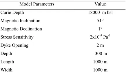
Table 1.1 – Pressure source geometry and medium properties.
Model Parameters Value
Curie Depth 18000 m bsl
Magnetic Inclination 51°
Magnetic Declination 1°
Stress Sensitivity 2x10⁻⁹ Pa-1
Depth -1500 m bsl
Radius 500 m
Xc 500 UTM km
Yc 4178 UTM km
For the computation of the piezomagnetic field change, it is assumed that the direction of the initial magnetization is the same as that of the geomagnetic field (I=51° and D=1°). The remanent magnetization of rocks of Etna, that were emplaced about 0.50 Ma (Branca et al., 2007) after the last field reversal (0.78 Ma; Tauxe et al., 1992), is generally much greater than induced magnetization (Königsberger ratio is > 1; see e.g. Rolph, 1992; Tric et al., 1994). Considering the Curie temperatures, which for Etna’s rocks were generally found near TC 550°C (Del Negro and Ferrucci, 1998), and a vertical geothermal gradient of 30 °C/km measured in deep boreholes (AGIP, 1977), we set the depth of the Curie isotherm at 18 km bsl.
The numerical solutions of a homogeneous magneto-elastic half-space are compared with the analytical ones. The analytical solutions of the elastostatic and magnetic problems are obtained using the simple and common Mogi model embedded in a homogeneous Poisson’s medium (Mogi, 1958; Sasai, 1991b). We report on the changes in the north component (ΔX), in the east component (ΔY), and in the vertical component (ΔZ) of the magnetic field. We also computed the total magnetic field intensity (ΔF) defined as:
I Z I D Y I D X
F cos cos sin cos sin
(1.16)
since it is the parameter measured by scalar magnetometers that are usually installed in volcano monitoring networks (Del Negro et al., 2002). The piezomagnetic variation is evaluated at a height of 4 m from the ground surface, the height of the magnetic sensors installed on Etna volcano.
A good match between the analytical and numerical solutions (model A) is obtained (Fig. 1.4).
Figure 1.4 – Comparison between the analytical solutions (color scale) and
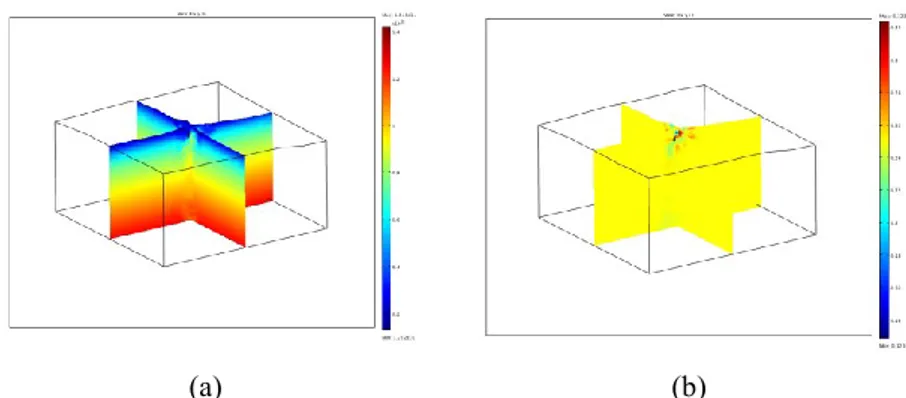
Then the gravity changes caused by the expansion of a spherical source embedded in a homogeneous Poisson’s medium (=) are compared with the analytical expressions (Hagiwara 1977). Since the different contributions to density variation (Eq. 1.14) are linearly summed in the Poisson’s equation, the three terms g1, g2 and g3 can be solved separately thanks to the superposition principle.
(a) (b)
(c)
Figure 1.5 Comparison between the analytical solutions (color scale) and the
We analyzed the case in which the source inflates without addition of new mass: V’’=V, where V and V’ are the source volume before and after the inflation respectively and and ’ are the source density before and after the inflation. In such a case the overall gravity change (g1+g2+g3) due to the deformation of an homogeneous half-space caused by a point source vanishes identically (Walsh and Rice, 1979). Numerical results well agree with the analytical ones (Fig. 1.5).
1.3.2 Piezomagnetic
and
gravity
field
generated by intrusive source
After having investigated pressure sources, we computed the numerical solution of piezomagnetic field and gravity field generated by intrusive source, that are the most common sources at Mt Etna. A classic mechanism of magma uprising is related to intrusive processes characterizing the emplacement of dikes. An intrusive dike is an igneous body with a very high aspect ratio, which means that its thickness is usually much smaller than the other two dimensions. A dike can be represented by an opening fault (tensile slip). Tensile dislocation theory has been applied with success to the case of a rectangular shaped source with tensile opening in an elastic homogeneous half-space (Okada, 1985; Yang and Davis, 1986).
In the numerical model the intrusion source is simulated as a discontinuity surface by introducing the mesh elements in pairs along the surface rupture. A given displacement in two opposite directions is applied at the two dike faces.
The source is located at the axis origin and it has an opening of 2 m, buried at a depth of 300 m (Table 1.2) in a homogeneous half-space medium whose medium parameters are the following: Young modulus E=50 GPa, Poisson’s ratio ν=0.25, initial magnetization J=8 A/m, density of rocks =2500 kg/m3.
Table 1.2 – Intrusive source geometry and medium properties.
Model Parameters Value
Curie Depth 18000 m bsl Magnetic Inclination 51° Magnetic Declination 1° Stress Sensitivity 2x10⁻⁹ Pa-1 Dyke Opening 2 m Depth -300 m Length 1000 m Width 1000 m
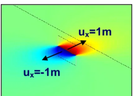
In Fig.1.6 it is showed the horizontal displacement at the dyke wall along a section of the domain at z=-800 m.
Figure 1.6 Displacement at the source wall along a section at z=-800 m in a
3D view. Red and blue colors represent the positive and negative displacement along the x-axis respectively.
Comparison between analytical (Utsugi et al. [2000] for magnetic field, Okubo [1992] for gravity field) and numerical solutions are performed to validate the numerical solution.
Figure 1.7 Comparison between the analytical solutions (color scale) and the
numerical results (line) of piezomagnetic variation generated by a dyke
u
x=1m
Figure 1.8 Comparison between the analytical solutions (color scale) and the
numerical results (line) of gravity variation generated by a dyke source. Contour lines are at 5uGal intervals.
Also for the piezomagnetic and gravity changes generated by an intrusive source there is a good match between analytical and numerical solutions, as showed in Fig. 1.7 and 1.8.
1.4 Discussions
Piezomagnetic and gravity fields produced by pressurized volcanic sources and dyke sources were evaluated by finite element models. The FEM allows us to consider a more realistic picture of volcanic framework by including (i) the topography, (ii) the magnetic heterogeneities of the medium and (iii) the elastic properties distribution. In this section we did not intend to interpret geophysical
changes at Mt Etna as those due to volcanic eruptions, but rather define the numerical model an test the accuracy.
Benchmark tests were carried out comparing the analytical and numerical results of piezomagnetic and gravity field both for pressure sources and intrusive sources.
Our findings highlight that the differential equations of ground deformation, magnetic and gravity field are solved with good accuracy with FEM model. The numerical model is able to represent the geophysical changes, with the possibility to include the complexity of the volcano structure, overcoming the limitations of analytical models.
Chapter 2
Effects of Heterogeneity and
Topography on Piezomagnetic
Field
The first attempts to estimate the effect of heterogeneity in rock magnetization were carried out solving a 2D numerical model for dislocation source (Zlotnicki and Cornet, 1986) and pressure source (Oshiman, 1990). Recently, Okubo and Oshiman (2004) derived a semi-analytical solution to assess the effects of layered elastic medium on piezomagnetic changes. These previous studies found that neglecting non-uniform distribution of either rock magnetization or elastic properties can introduce underestimations in the interpretation of piezomagnetic fields. Besides the medium heterogeneity, also the topography can alter the estimate of the piezomagnetic field. Using a
irregular piezomagnetic changes can arise in a 2D homogeneous medium because of local stress concentration on jagged topography. Using the Finite Element Method (FEM) Yamazaki & Sakai (2006) also observed that local piezomagnetic changes occur in presence of strong slope changes.
Although these previous studies have shown the role played by heterogeneity and topography on piezomagnetic fields, to date most of the models generally used in volcanic areas are based on analytical solutions. With the aim of considering a more realistic description of Mt Etna, we developed the FEM-based numerical model to solve the piezomagnetic field, including not only complicated distributions of both rock magnetization and elastic rigidity, but also the real topography of the studied area. In Currenti et al. (2007) several tests were carried out to appraise the influence of topography and medium heterogeneities on gravity field. In this chapter elastic finite element models are applied to investigate the effects of topography and medium heterogeneities on the piezomagnetic field produced by volcanic pressure sources.
We used the same computational framework described in the previous section for investigating the heterogeneity and topography effect. The source parameters are reported in Table 1.1. Initially, we studied the perturbations caused by the medium heterogeneity using different model parameters. Successively, we took the real topography of Mt Etna into account.
2.1 Heterogeneity effect
We investigated the effects of medium heterogeneity using different model parameters (Table 2.1). All the results can be compared to the model A in Table 2.1, that corresponds to the medium parameters of the homogeneous model whose results are reported in section 1.3.1.
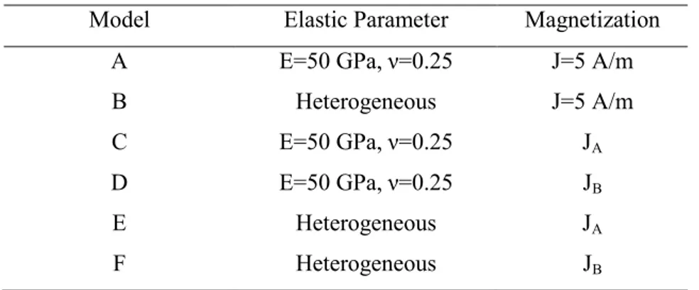
Table 2.1 – Model properties. The magnetic structures JA and JB are described in Fig. 2.3.
Model Elastic Parameter Magnetization
A E=50 GPa, ν=0.25 J=5 A/m
B Heterogeneous J=5 A/m
C E=50 GPa, ν=0.25 JA
D E=50 GPa, ν=0.25 JB
E Heterogeneous JA
F Heterogeneous JB
2.1.1 Effects of elastic heterogeneity
Firstly, we evaluated the effect of elastic heterogeneity on the piezomagnetic field while the magnetic properties are assumed homogeneous (model B). A medium for the subsurface structure of Mt Etna is considered by assigning the elastic material properties derived from seismic tomography data to the domain (Patané et al., 2006). We used P-wave and S-wave seismic velocities to define the Young
1 1 2 1 V E 2 p (2.1)where Vp is the seismic P-wave propagation velocity, and is the
density of the medium, which was set at an average value of 2500 kg/m3 (Corsaro and Pompilio, 2004). Instead, the values of Poisson’s ratio were obtained using the equation (Kearey and Brooks, 1991):
]
2
)
/
(
2
/[
]
2
)
/
[(
2
2
V
pV
sV
pV
s
(2.2)where Vs is the seismic S-wave propagation velocity. On the basis of
Eqs. (2.1) and (2.2), within the computational domain the Young modulus varies from 11.5 GPa to 133 GPa, while the Poisson ratio is in the range 0.12-0.32.
(a) (b)
reference surface at 1500 m asl, which represents the average altitude of Etna’s topography, is considered. Therefore, in the numerical models the source is positioned at 1500 m bsl with a relative distance from the reference surface of 3000 m, as in the analytical model. The amplitude of the piezomagnetic field does not change significantly with respect to the homogeneous model. Only a slight change in the shape is observed due to smooth variations in the elastic parameters (Fig. 2.2a).
Figure 2.2 –Total intensity of piezomagnetic field produced by a pressure
change (a) and a volume change (b) in a spherical source for the half-space model B, which is homogeneous in magnetic properties and heterogeneous in elastic parameters. Contour lines are at 0.5 nT intervals. The star represents the pressure source location.
structure can be attributed to the assumption of a pressure change at the source wall instead of a volume change as in Okubo and Oshiman (2004). The stress and the piezomagnetic fields produced by a center of dilatation (COD) coincide with those generated by a center of pressure (COP) in a homogeneous elastic half-space (A model) where the pressure change can be related to the volume change through the Lamé constants (Currenti et al., 2008c). The piezomagnetic solution is proportional to the moment of strain nucleus C that can be expressed in terms of V or P as: P a V C 2 2 3
(2.3)where a is the radius of the source. As confirmed by the inspection of the analytical solutions in Sasai (1991), the COP model does not depend on the rigidity modulus, whereas the COD model is linearly related to it. While in the COP model the piezomagnetic field is dependent on the intensity of the pressure applied at the source wall, in the COD model the piezomagnetic field is lower for a softer medium and higher for a stiffer medium. To assess the differences between COD and COP models in heterogeneous elastic medium, we computed the model B also for a COD model having the same volume increase as the COP model (Fig. 2.2a). The comparison between the COD and COP models shows significantly different results, indicating that the COD model is more sensitive to the elastic rheology (Fig. 2.2b). These results are in agreement with those obtained by Okubo
changes in the piezomagnetic field when boundaries of elastic layers are near to the source. The stress change in the COD model, and thus the piezomagnetic change, is strongly influenced by the elastic parameters. While the heterogeneity slightly affects the model in which the pressure change is assigned, it alters the solution when a volume change of the source is considered. Whether an intrusion process is better described in terms of a pressure source or of a volume change probably depends on the rheology of the medium. However, it is worth noting that for an elastic rheology a growth of magma chamber is better described in terms of pressure change than volume change, since the volume increase is indeed the resulting effect of source pressurization.
2.1.2 Effects of magnetic heterogeneity
Successively, models with heterogeneous distribution of initial magnetization, but homogeneous in elastic properties were also investigated (models C and D). Generally, in a volcano such as Etna, built up by a stack of basic lavas, magnetizations are irregular and frequently high (Hildenbrand et al. 1993). The magnetic properties of volcanic rocks cropping out in the Etna volcano have rarely been measured; however the few laboratory measurements carried out on recent and historic lava flows confirmed high values of remanent magnetization (JNRM) ranging between 9.4 and 1. 4 A/m (Pozzi, 1977;of Mt Etna, recently collected from lava flows and dikes, revealed an average JNRM of 7 A/m with the highest values associated to dikes,
while the lower ones related to volcaniclastic deposits (Del Negro and Napoli, 2002). Therefore, we assumed a high magnetization value for the volcano edifice lying on a substrate with lower magnetization. In particular, we considered two half-spaces with different layers and magnetic properties, thereafter referred as JA and JB (Fig. 2.3).
Figure 2.3 – Layered structures of the initial magnetization free from
stresses. On the left the JA two-layered magnetization structure, on the right the JB three-layered magnetization structure.
Lateral heterogeneities are disregarded since they are poorly known and could alter the solutions. In the two-layered half-space JA, we
assume a value of the initial magnetization free from stresses Jo=8
A/m from ground surface to 0 m asl, reproducing the magnetization of the rocks in the volcano edifice. A lower value of Jo=5 A/m is
depth due both to the presence of areas with temperatures greater than Curie temperature and hydrothermal alteration occurring in zones surrounding magma storage or emplacement. Depth dependence is used to explain the loss of initial magnetization associated with the geothermal gradient, given by the following equation in SI units (Zlotnicki and Cornet, 1986; Stacey and Banerjee, 1974):
03 . 0 10 0 03 . 0 10 / ) 10 ) ( 03 . 0 ( 1 0 0 2 0 0 c c c T z z T z z T z z J J (2.4)where Tc=590 °C is the Curie temperature in degree Celsius, 0.03
°C/m the geothermal gradient, 10 °C the temperature at ground surface, z0=1500 m the reference level and z is the depth in meters. The simple two-layered model JA, is an over-simplification of the
variation of magnetization in the Etna subsurface. However, the intensity of magnetization can vary widely within volcanic edifice, because of changes in composition, grain size, and concentration of magnetic minerals (Rosenbaum, 1993). Considering the tomographic modelling of Etna plumbing system obtained by Chiarabba et al. (2000) and the geology-based models by Tibaldi and Groppelli (2002) (Fig.2.4), we also evaluated a three-layered half-space structure JB.
Figure 2.4 - Geological based model of Mt Etna by Tibaldi and Groppelli.
The first layer is the same as for the structure JA. The second layer
extends from 0 to 3 km bsl depth with a magnetization value of Jo=3
A/m. This lower value of Jo was speculated because of the presence of
the regional apenninic structure, composed mainly of sedimentary rocks, surrounding and hosting the main intrusive bodies, and crystalline and metamorphic basement. Moreover, this layer is generally interpreted as the region where the magma is preferentially stored before the recent eruptions (Budetta et al, 2004; Bonaccorso and Davis, 2004; Bonforte et al., 2008). Here, the magma accumulation laterally extends for about 10 km, but the presence of hot fluids circulating around the shallow magma reservoir produce high values of temperature in a larger area (De Gori et al., 2005). The magnetization of the third layer, which starts from 3 km bsl, is assumed depth dependent following the Eq. (2.4). To this layer we associated an initial magnetization of Jo=8 A/m due to the presence of
magnetization show that the shape of the variation is strongly dependent on the assumed magnetic structures (Fig. 2.5).
Figure 2.5 – The total piezomagnetic field for the half-space models C (a)
and D (b). Contour lines are at 0.5 nT intervals.
In the heterogeneous model D both the shape and the amplitude of the expected magnetic field are perturbed (Fig. 2.5b). The comparison with the analytical solutions (Fig. 1.4) shows that the maximum values of the positive piezomagnetic changes reach 2.8 nT and 1.2 nT for the models C and D, respectively. Indeed, the piezomagnetic changes depend almost entirely on the stress-induced magnetization of the medium surrounding the source (Davis, 1976). In the heterogeneous model C the pressure source is surrounded by an average magnetization which is almost equal to that of model A and the
contrary, in model D a lower initial magnetization (3 A/m) is assumed around the source and a decrease in the piezomagnetic field is observed at ground surface with respect to the homogeneous model (A). A difference of about 1.5 nT in the negative polarity of the magnetic field is observed in the model D, where the amplitude of the negative polarity exceeds that of the positive one.
Both elastic and magnetization heterogeneities are then included in the models E and F with magnetization layers JA and JB, respectively (Fig.
2.6).
Figure 2.6 – Total intensity of piezomagnetic field (contour lines at 0.5 nT
the amplitude of the piezomagnetic field with respect to the elastic homogeneous models C and D. Only the shape shows small changes, just as occurred in the elastic heterogeneous model B.
2.2 Topography effect
To estimate the effect of topography on piezomagnetic fields, we included the real topography of Mt Etna in the previous models. The ground surface was generated using a digital elevation model of Mt Etna from the 90 m Shuttle Radar Topography Mission (SRTM) data and a bathymetry model from the GEBCO database (http://www.gebco.net/) (Fig.2.7).
Figure 2.7 - Mesh of the topography of Mt Etna.
The computational domain was meshed into 152,859 isoparametric, and arbitrarily distorted tetrahedral elements connected by 26,090 nodes.
The medium is initially assumed to be homogeneous in elastic and magnetic properties in order to estimate the differences due to the topography separately. A change in shape is clearly observed in the