Crustal structure and dynamics in southeastern Sicily (Italy) by using seismological data.

UNIVERSITÀ DEGLI STUDI DI CATANIA

Dipartimento di Scienze Biologiche, Geologiche e

Ambientali, Sezione Scienze della Terra

DOTTORATO

DI

RICERCA

IN

GEODINAMICA

E

SISMOTETTONICA

CICLO XXV

CRUSTAL STRUCTURE AND DYNAMICS IN

SOUTHEASTERN SICILY (ITALY) BY USING

SEISMOLOGICAL DATA

Dott.ssa Carla Musumeci

Coordinatore

Prof. Carmelo Monaco

Tutor Co-tutor

Prof. Stefano Gresta Prof. Stefano Catalano

“Un vincitore è semplicemente un sognatore che non si è mai arreso.” “A winner is just a dreamer who never gave up.”

Abstract 1

Chapter 1 2

Introduction 2

Chapter 2 5

2.1 Geological Setting of Southeastern Sicily 5

2.2 Previous Geophysical Studies 8

2.2.1 DSS profiles 9

2.2.2 Tomographic models 13

2.2.3 Recent Receiver Function studies and Local Seismicity 17

Chapter 3 21

3.1 Methods 23

3.1.1 P-to-S receiver function method 23

3.1.2 Estimation of crustal thickness and VP/VS ratio 29

Chapter 4 32

4.1 Data and Methods 32

4.2 Data Examples and Crustal Thickness Calculation 38

4.2.1 Results by Stations 39 4.2.1.1 SSY 39 4.2.1.2 HCRL 47 4.2.1.3 HAGA 54 4.2.1.4 HVZN 59 4.2.1.5 HMDC 65 4.2.1.6 HAVL 71 4.2.1.7 HLNI 77 4.2.1.8 RAFF 83 Chapter 5 87

5.1 Results and Conclusions 87

Chapter 6 96

6.1 Concluding remarks 96

Acknowledgments 101

References 102

Abstract

Introduction: Through receiver function analysis, this study inquires into some of the

most basic properties of the crust below southeastern Sicily (Italy), mostly represented by the Hyblean Plateau. Method: This is accomplished, using P-to-S receiver function (P-RF) technique which involves coordinate rotation and deconvolution, by stacking waveforms from 335 teleseismic events, magnitude 6.0 and larger, to determine the delay in arrival time for several phases of the P-wave coda, relative to the initial P-wave arrival. This information is used to establish a linear relationship between thickness and VP/VS ratio, each of which is stacked using the slant stacking approach for a given

station to identify the best-fit thickness and wave speed for the crust below that station. To determine their accuracy these results are compared with previous studies, as well as with synthetically generated receiver functions based on 1D crustal models including dipping layers. Results: The good regional coverage and the fairly dense station spacing (~20 km) leaded to a fairly complete image of the crust-mantle boundary over the entire region that shows strong lateral variations of the crustal thickness with Moho depth varying between 29 and 38 km. In particular, a thinner crust is observed in the central-eastern part of the Hyblean Foreland beneath SSY (Solarino) station and thickening further to the south beneath HMDC (Modica) station (up to 38 km) and to the north beneath HLNI (Lentini) station (up to 35 km). Sharp transitions between thinned and thickened crust are most likely the result of complicated 3D structures attributed to regional geodynamics. Discussion: Since all the 8 considered broadband stations lie in a geodinamically complex area, reliable estimates of the crustal thicknesses below these stations are key requisite for understanding the geologic and tectonic processes that have been dominant in the region, providing valuable information for the numerous earth science disciplines.

Chapter 1

Introduction

The structure of the Earth’s interior is fairly well known from seismology, and knowledge of the fine structure is improving continuously. Seismology not only provides the structure, but also gives information about the composition, crystal structure or mineralogy and physical state.

Earth is conventionally divided into several distinct layers (crust, mantle and core), considered as a system of horizontal layers affecting the seismic energy arriving at a given station (Fig. 1). Only the uppermost part of the crust is available for direct sampling from boreholes. At greater depths all information about its composition and structure is indirect.

Fig. 1- Simplified structure model of the Earth.

Much of the information about the Earth’s interior has been derived from the knowledge of the variation of seismic velocities with depth. Consequently, the recorded motion at the earth’s surface depends on the elastic parameters, the thickness of these layers, as well as on the existing seismic energy and the recording instrument.

The reconstruction of the Earth’s interior, from geophysical observables recorded at the surface, is called an ‘inverse problem’. Inverse problem theory has been widely developed in geophysics from earthquakes locations to seismic tomography (Tarantola, 1987; Zhang and Thurber, 2003). One of these inverse problems is the reconstruction of a vertical profile of the elastic properties at depth under a seismic station using P-to-S converted phases generated at subsurface discontinuities (Langston, 1979). With regard

to this, receiver functions (RFs) are time series that contain P-to-S phases, and are computed from teleseismic recordings through the deconvolution of the vertical component of a teleseismic waveform from the horizontal ones. The solution of the RF inverse problem involves locating subsurface seismic discontinuities, reconstructing the elastic properties in the subsurface, and estimating the uncertainties associated with these quantities (Piana Agostinetti and Malinverno, 2010).

The first accurate teleseismic recording was obtained in 1889 in Potsdam (Germany), 15 minutes after an earthquake in Japan (von Rebeur-Paschwitz, 1889), while the beginning of the systematic collection of global seismic data was started in 1892 by John Milne (Milne, 1895). Teleseismic body waves have been used extensively for a long time to retrieve crustal and lithospheric structures beneath recording stations (Phinney, 1964) under the name of ‘Crustal Transfer Method’. The method has been subsequently improved by several workers (e.g. Burdick and Langston, 1977; Owens et alii, 1984). It is now commonly referred to as the ‘Receiver Function Method’, one of the most widely used technique to determine the crustal structure on a regional scale below the recording stations. For this reason, teleseismic receiver functions have been often used to locally determine depth and dip of crustal and upper mantle discontinuities for peninsular Italy (Piana Agostinetti et alii, 2002; Mele and Sandvol, 2003; Lucente et alii, 2005; Margheriti et alii, 2006; Piana Agostinetti and Amato, 2009; Miller and Piana Agostinetti, 2012). Southeastern Sicily, one of the most seismically active areas of the Mediterranean Basin, is poorly covered by these studies. The complex tectonic history and the active tectonics of this region motivated the present research to look at the crustal structure beneath single seismic stations, to infer some more elements useful for geodynamic reconstructions and to infer any correlation between the deeper structure and the surface tectonics. Specifically, the research of this PhD project consisted in the application of the P-to-S receiver function (P-RF) analysis technique to investigate the crustal thickness in southeastern Sicily (Italy), in order to increase the spatial resolution of the Moho maps of the region. This study considered seismograms recorded at 8 broadband stations, deployed in the investigated area, all of which are part of the seismic permanent network currently operated by the Istituto Nazionale di Geofisica e Vulcanologia (INGV, Osservatorio Etneo, Sezione di Catania). These stations overlie several interesting geological provinces in the region, covering Recent Quaternary deposits, Plio-Pleistocene Hyblean volcanics, Appennine-Maghrebian units and Meso-Cenozoic carbonate sediments. Estimates of crustal thickness below these stations are

useful in characterizing the “topography” of the crust-mantle interface, key requisite for geodynamic modelling, for understanding the evolution and state of lithosphere, enhancing the understanding of how ancient tectonic events continue to shape and define the structure of our continent.

Firstly, all previous studies in the area have been reviewed in details to give a starting point to the analysis and to better define the previous knowledge about the seismic structure in this region. Then, the results are discussed, comparing them with previous findings and discussing some original implications for the geological evolution. In particular this manuscript is organized as follows:

 Chapter 2 summarizes the geological and tectonic setting of the investigated area, whose knowledge is important for successive correlations with the analysis results. Instrumental and historical seismicity are also presented in this chapter and the previous geophysical studies are briefly introduced.

 Chapter 3 discusses the receiver function method and describes the different steps of data processing.

 Chapter 4 introduces the dataset. Here, data examples are presented, as well.  Chapter 5 shows the results in terms of crustal thickness.

 Chapter 6 presents the concluding remarks of this research and the critical conclusions are here discussed. Additional information on the selected events are in Appendix A.

Chapter 2

2.1 Geological Setting of Southeastern Sicily

From a geological point of view, southeastern Sicily is an area of great interest because: 1) it represents an important piece of the collision front between Nubia and Eurasia; 2) it is very close to the biggest European volcano Mount Etna and, 3) it has been hit by strong earthquakes in the past (1169, 1542 and 1693) that struggled the cities of Catania, Siracusa and Ragusa provoking tens of thousands of casualties.

Its geological-structural setting must be considered in the frame of the complex tectonic features of the Mediterranean basin, which is dominated by the ~N20°W Neogene-Quaternary convergence between Nubian plate (the African plate west of the East African Rift) and Eurasia, occurred in the last 100 million years (Faccenna et alii, 2001). Tectonic forces resulting from the relative movements among these plates are transferred into the continental crust, where large structures, as subduction thrusts, major faults and normal detachments, accommodate most of the strain and produce nearly all of the most destroying earthquakes. Regionally speaking, in the whole region of Sicily we may distinguish a northern imbricate mountain chain (Appenninic-Magrebian Chain or Maghrebian Thrust Belt), a deep Neogene basin filled with nappes (Caltanissetta Basin) and a relatively stable carbonate platform to the southeast (Hyblean Plateau) (Fig. 2). The evolution of these units can be correlated with two main tectonic phases: (i) a mid Triassic to Cretaceous extensional phase, related to Tethyan rifting; (ii) a Tertiary to recent compressional phase during which the Sicilian segment of the North African continental margin has been affected by continental collision. The extension created horst/graben platforms and basins which were subsequently deformed and overthrusted during the later compressional phase (Catalano et alii, 2010).

Southeastern Sicily is mostly represented by the Hyblean Plateau, a distinct crustal unit located at the northeastern end of the mostly submerged Pelagian Block (Burollet et alii, 1978). The autochthonous sedimentary wedge (about 7 km thick) overlies an “African” continental crust and consists of thick Triassic-Liassic platform and slope-to-basin carbonates, overlain by Jurassic-Eocene pelagic carbonates and Tertiary open shelf clastic deposits (Patacca et alii, 1979; Bianchi et alii, 1987; Grasso et alii, 2004), with intercalated Plio-Pleistocene mafic volcanics at several distinct intervals (Grasso et alii, 1983). Its crustal structure and gravimetric and magnetic anomalies differ from those of adjacent areas of the African Foreland. At the present, the plateau plays the role of a crustal indenter that, confined between the flexured continental thinned-crust area

of the Caltanissetta Basin, to the west, and the oceanic domains of the Ionian Basin (Finetti and Del Ben, 1996), to the east, has impinged against the front of the Maghrebian Thrust Belt (Fig. 2).

Fig. 2- Tectonic sketch map of the Central Mediterranean from Tunisia to the Calabrian

arc, showing the main Quaternary fault belts and their relation with plate boundaries and incipient rift zones. The inset describes the location of the Nubia-Eurasia convergent plate boundary and of the divergent western margin of Adria. Focal mechanisms are from Anderson and Jackson (1987) and Pondrelli et alii (2002-2004) and GPS velocities are from Hollestein et alii (2003) and D'Agostino and Selvaggi (2004). (From Catalano et alii, 2010).

The northern and western margins of the Hyblean Plateau are characterized by an older extensional belt (named Gela-Catania Foredeep), that forming a roughly NE-SW alignment, is downbent by a NE-SW fault system under the front of the Appenninic-Maghrebian Thrust Belt (Yellin-Dror et alii, 1997). This narrow and weakly deformed depression (Gela Basin) developed from the Late Pliocene onwards, as suggested by biostratigraphic analyses, and is probably related to the inflection of the carbonate

substrate due to the frontal nappe loading. The basin fill consists of Plio-Pleistocene pelagic marly limestones, and sandy clays unconformably overlying the Messinian evaporites.

To the east, the plateau is indeed bordered by the Malta Escarpment fault system (MEFS) (Fig. 2), one of the largest normal fault systems of the Mediterranean basin (e.g., Reuther et alii, 1993; Adam et alii, 2000). Regionally, this normal NNW-SSE trending lithospheric fault system extends from 15 to 50 km offshore and over a length of about 300 km from the eastern coast of Sicily southwards, showing a steep slope that steps down rapidly from 200 m to more than 3000 m below sea level and a width of about 40 km (Ben-Avraham et alii, 1995; Lanzafame and Bousquet, 1997). Since the late Cretaceous onset of African and Eurasian plates convergence, the Malta Escarpment fault system has been converted from a Mesozoic passive margin into a mega-hinge fault system, with an additional sinistral strike-slip component. Since the Pleistocene, sinistral strike-slip deformation and simultaneous normal faulting along this lithospheric fault system have induced the opening of oblique trending onshore grabens at the eastern margin of the Hyblean Plateau (Adam et alii, 2000). According to Bianca et alii (1999) and Azzaro and Barbano (2000), the Malta Escarpment fault system is responsible for the primary seismic activity of the region. Major historically (February 4, 1169; January 11, 1693) destructive earthquakes (M=7) occurred along this fault system (Azzaro and Barbano, 2000), causing tens of thousands of casualties. Weaker shocks (M<6) are due to secondary inland faults striking along an overall NE-SW and NNE-SSW direction (i.e., Scordia-Lentini Graben, Rosolini-Pozzallo and Scicli-Ragusa fault systems). The more recent seismicity of the area is characterized by earthquakes, with magnitudes less than ML 4.6 (Musumeci et alii, 2005). Zones characterized by nil

seismicity involve the central part of the Foreland. In depth, seismicity generally extends to about 30 km, with foci mainly concentrated from 15 to 25 km (Musumeci et alii, 2005). Earthquake focal mechanisms inferred for the study area are characterized by a predominance of normal fault-plane solutions along the Malta Escarpment, and mainly by strike-slip solutions with lesser amounts of both normal and reverse faulting in the plateau. The inversion of these fault plane solutions coherently results in stress tensors which constrain an active NW-SE to NNW-SSE oriented regional compression (Musumeci et alii, 2005).

2.2 Previous Geophysical Studies

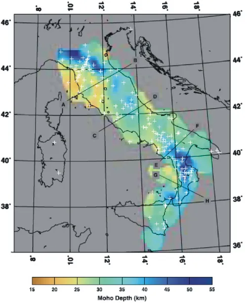
In complex tectonics regions, seismological, geophysical and geodynamic modeling require accurate definition of the Moho geometry. Maps of the Moho topography beneath Italy have been published over the years, based on results from different geophysical methods. Morelli et alii (1967) introduced preliminary isobaths for the Moho in Europe. Geiss (1987) produced a map of the Moho topography at the Mediterranean scale, through a least square interpolation of a large number of different geophysical observations. Nicolich and Dal Piaz (1991) presented a simplified sketch map of the Moho isobaths for the Italian region, based only on controlled source seismology (CSS) data. Suhadolc and Panza (1989) and Scarascia et alii (1994) published compilation maps of the Moho isobaths for the European and Italian areas respectively, both based on revised interpretations of CSS profiles. Du et alii (1998) produced the EurID 3-D regionalized model of the European crust and mantle velocity structure including a map of the Moho depth obtained by compiling results of several CSS investigations performed in the area. Pontevivo and Panza (2002) defined the characteristics of the lithosphere-asthenosphere system in Italy based on the analysis of Rayleigh wave dispersion. Piana Agostinetti and Amato (2009) compiled the map of the Moho depth for the Italian peninsula using P receiver functions. Grad et alii (2009) produced a map of the Moho depth beneath Europe based on seismic and gravity data. Waldhauser et alii (1998) proposed a new method to determine the 3D topography and lateral continuity of seismic interfaces and a mean P wave 3D velocity model by using 2D-derived CSS reflector data. Di Stefano et alii (2011) presented a map of the 3D Moho geometry obtained by integrating high-quality CSS data and teleseismic receiver function data. Miller and Piana Agostinetti (2012) investigated the lithospheric structure using S receiver functions. Looking at southeastern Sicily, previous studies on Moho depth geometry have been documented by papers based on wide-angle DSS profiles, gravimetric modeling, deep reflection profiles, receiver function studies and seismic tomography (e.g., Scarascia et alii, 1994; Scarfì et alii, 2007; Piana Agostinetti and Amato, 2009; Miller and Piana Agostinetti, 2011). Although the main features outlined by these studies are robust, large uncertainties are whatever present in the seismic models as an effect of different acquisition and interpretation techniques and/or due to the complexities of the tectonic settings in the area of investigation. A brief review of the main results so far are given in the following sections.

2.2.1 DSS profiles

The seismic exploration method of wide angle reflection-refraction, generally known as Deep Seismic Soundings (DSS), were performed in the Italian peninsula by a cooperation of French, German, Swiss and Italian geophysical research institutions. In particular, under the sponsorship of the European Seismological Commission and the Explosion Seismology Group from 1956 to 1982 and through the European Science Foundation and the European Geotraverse from 1983 to 1989. It has to be called that the only physical parameter that can be determined (with variable accuracy) is the velocity of the P waves. Therefore, petrological and rheological models can be derived only through the assumption of hypotheses on rock composition and with the help of complementary data, like the heat flow. Furthermore, since the maximum depth of the DSS is limited to the crust-mantle boundary, little information was obtained on the continuation with depth of the tectonic structures below that limit.

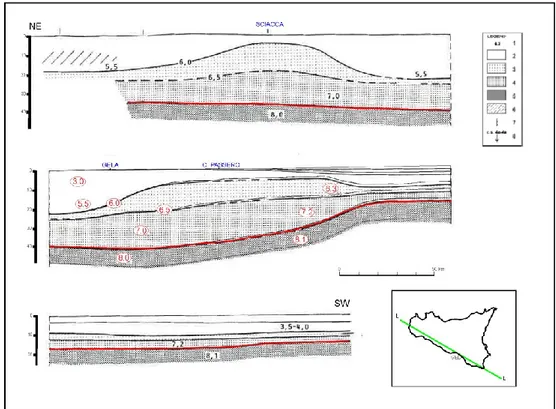
A description of the techniques of acquisition and processing of the DSS data is out of the scope of this thesis and the discussion is just limited to show the different interpretations and the subsequent modifications that were brought (if they are). In particular, the crust-upper mantle structure of the southeastern Sicily was investigated by the analysis of two DSS profiles acquired during 1984. For the sake of clarity, to the DSS cross sections are assigned the same number and letters that were used in Scarascia et alii (1994) (Fig. 3), in Continisio et alii (1997) (Fig. 4) and in Cassinis et alii (2003) (Fig. 5).

Cross section L-L in Fig. 3, along the western coast of Sicily, is located between Egadi Islands and Capo Passero, and extends to the SE towards the Ionian abyssal plain. The part of the section under Sicily was explored by using shots located in the sea near Egadi, Gela and Capo Passero and recorded by land stations. The sea tract was explored with OBS and closely-spaced shots located in the Ionian Sea. The profile is characterized by significant lateral depth changes of both the Moho and the intracrustal interface (Scarascia et alii, 1994). Along the SW Sicilian coastline the thickness of the crust ranges between 35 and 40 km and the shallow layers reach a remarkable thickness (20 km).

The reconstruction of the crustal sections shown in Fig. 4 comes from the interpretations of Continisio et alii (1997). The profile c (Fig. 4), acquired along the southern coast (DSS profile as above) crosses the Sicily in a WNW-ESE direction from Marsala on the western coast to Capo Passero on the southern one. In the Caltanissetta

trough, the Moho depth (blue line) reaches 35 km. Beneath the Hyblean Foreland the Moho rises to about 30 km. In the Hyblean Foreland, upper crust velocities of 5.4 km/s were needed for fitting the data. This feature can be accounted for by the thick sequences of rocks with large bulk moduli as those (carbonatic and volcanic) found by drill-holes in the Hyblean area (e.g. Longaretti and Rocchi, 1990).

Fig. 3- Interpretative cross-section Egadi Islands-Capo Passero-Ionian Sea. Legend:

1=Velocities in km/s; 2=Surface layers (V<6.0 km/s); 3=Upper or undifferentiated crust (V=6.0-6.5 km/s); 4=Lower crust (6.5-7.5 km/s); 5=Upper mantle (V>7.5 km/s); 6=Low velocity layers; 7=coastline. (From Scarascia et alii, 1994).

The profile b (Fig. 4), acquired in the central Sicily (striking NNE-SSW), starts near Milazzo, on the Tyrrhenian coast, crosses the Sicilian-Maghrebian chain in the north, the Caltanissetta trough in central Sicily, and ends on the southern coast near Gela, close to the outcroppings of the Hyblean plateau. The crustal structure (Continisio et alii, 1997), is characterized by a Moho depth (red line) of less than 20 km offshore the northeastern margin of Sicily, in the Tyrrhenian sea, 30 km beneath the Peloritani chain, and 35 km in the Caltanissetta trough. In the Gela-Catania Foredeep the Moho rises to 22 km, whereas in the Hyblean Foreland it reaches 30 km. The main Moho flexure zones along the profile are located beneath each transition from one major structural domain to another (Tyrrhenian Sea-to-Chain, Chain-to-Foredeep and Foredeep-to-Foreland).

Fig. 4- Location of the DSS profiles (b and c) and interpretative

cross-sections. (From Continsio et alii, 1997).

Recently, the processing and interpreting work was continued through new procedures (digitalization of the old analogically-recorded data, use of synthetic seismograms, seismic modeling). Thus updated interpretations of individual cross sections and more detailed maps of the Moho boundary were proposed. Section 12-12 (Fig. 5) from Cassinis et alii (2003) confirmed a crust-mantle discontinuity at depth of about 35-40 km beneath southeastern Sicily.

Fig. 5- Interpretative cross-section. Legend: (1) Velocities in km/s; (2; blue) Surface

layers (V<6.0 km/s);(3; green) Upper or undifferentiated crust (V=6.0-6.5 km/s); (4; fuchsia) Lower crust (6.5-7.5 km/s); (5; gray) Upper mantle (V>7.5 km/s); 6) Low velocity layers; 7) coastline. (From Cassinis et alii, 2003).

In this image the velocity ranges that characterizes the studied area have been shaded differently: the shallower layers, with velocity below 6.0 km/s, are in blue; green area indicates layers with velocity values ranging from 6.0 to 6.5 km/s (upper crust); fuchsia area indicates layers with velocity values ranging from 6.5 to 7.5 km/s (lower crust); gray area indicates upper mantle layers, with velocity values over 7.5 km/s.

Fig. 6 shows the Moho-depth contour map obtained by the synthesis of all data available in the Italian Seas and adjacent onshore areas (Cassinis et alii, 2003). In particular, the central-southern Sicily is characterized by a total thickness ranging between 22 and 40 km.

Fig. 6- Depth contour-lines of the Moho boundary. Contour interval 2.5 km. (From

Cassinis et alii, 2003, see the text for the legend and a detailed description).

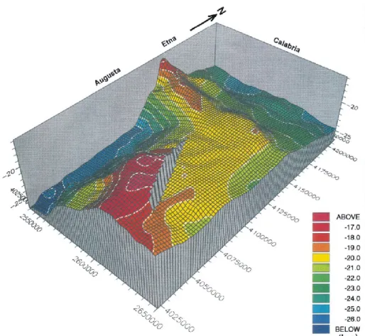
The thickness of the crust under eastern Sicily and the Moho topography beneath the Ionian Sea has been reinterpreted by Nicolich et alii (2000). The Authors used the results of the processing of an augmented grid of profiles at sea tying in all the Etna profiles and the Streamers Ionian profiles (Cernobori et alii, 1996) with

offshore-onshore wide angle control, in order to distinguish elements of the whole structure of the crust. Looking from the basin towards land (Fig. 7), the Moho deepens both towards Calabria in the north and Sicily in the south-west with depth of 30 km beneath the central Hyblean Plateau, rising to 22 km in the Gela-Catania Foredeep and to 21-18 km just offshore Catania (Nicolich et alii, 2000). Towards Calabria the Moho depth resumes a value on the order of 25 km or greater.

Fig. 7- Perspective view of Moho topography looking from the Ionian basin to NNW.

Etna is located on the NW prolongation of the mantle upwarp. (From Nicolich et alii, 2000).

For further regional geological and geophysical profiles across Sicily see also Bello et alii (2000), Chironi et alii (2000), Finetti (2005), La Vecchia et alii (2007) and reference therein.

2.2.2 Tomographic models

Among the tomographic models available for the area, those of Scarfi et alii (2007) and Brancato et alii (2009) are the most recent ones. Descriptions of the velocity structure in the crust-upper mantle are provided below.

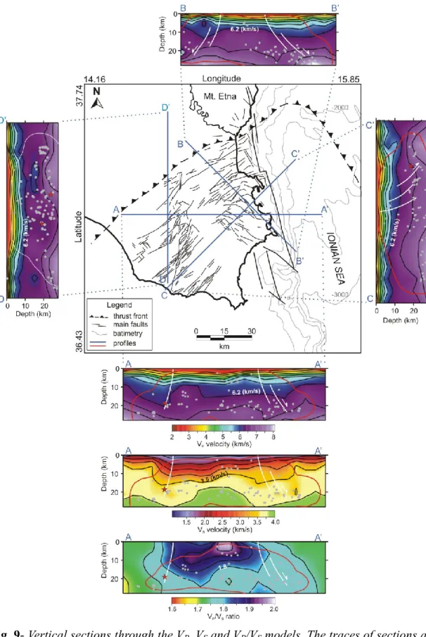
Scarfì et alii (2007) applied the adaptive mesh double difference tomography (Zhang and Thurber, 2005) to determine three dimensional VP, VS and VP/VS variations and

event locations in southeastern Sicily (Italy). P-wave velocity (VP) values ranged from

2.0 to 5.0 km/sec in the upper crust, increasing to ≥6.0 km/sec in the deeper crust (Figs. 8 and 9).

Fig. 8- VP (a), VS (b) and VP/VS (c) models for six representative layers resulting from

the 3D inversion. Contour lines are at interval of 0.5 km/s for VP and VS, and 0.05 for

VP/VS. On the 0 km layer the main structural features are reported with white lines.

Grey circles (ML<3.5) and red stars (ML≥3.5) represent the relocated earthquakes

within half the grid size of the slice. The zones with DWS>100 (a) and DWS>50 (b and c) are circumscribed by white contour lines. (From Scarfì et alii, 2007).

Fig. 9- Vertical sections through the VP, VS and VP/VS models. The traces of sections are

reported in the sketch map (AA’, BB’, CC’ and DD’). Contour lines are at an interval of 0.5 km/s for VP and VS, and 0.05 for VP/VS. Red curves contour the zones with

DWS>100 for VP and DWS>50 for VS and VP/VS. White lines indicate the main

structural features (the geometry of the fault planes are purely an indication). Relocated earthquakes, within ±10 km from the AA’, BB’, CC’ sections and within ±20 km from the DD’ section, are plotted as grey circles (ML<3.5) and red stars (ML≥3.5). (From Scarfì

A high VP/VS anomaly of 1.8-2.0, mainly corresponding to a low VP and VS zone, is

imaged in the central region down to a depth of 16 km. The high VP/VS anomaly has

been interpreted in terms of increase of crack density and presence of saturated fractures, which may decrease both P- and S-wave velocities and increase VP/VS ratios.

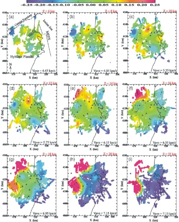
Map views from Brancato et alii (2009) are shown in Fig. 10.

Fig. 10- Depth slices through the tomographic seismic velocity model (smoothed

10×10×4 km). Triangles indicate seismic stations. (a) The surface locations of major fault systems and thrust fronts (seismic stations are removed for clarity). Earthquakes within 1 km above and below each slice are shown as black dots. The average velocities are also indicated in the bottom corner of each panel. The colour scale bar, at the top, represents the deviation from average velocities (in km/sec). Depths (Z) are relative to the sea level. (From Brancato et alii, 2009).

Depth slices through the tomographic seismic velocity model show that down to a depth of 10 km the average VP is relatively low (≤5.35 km/sec; Fig. 10c). For depths

greater than 10 km, average velocity increases from 5.35 to 7.15 km/sec, then remains relatively constant below 20 km (Fig. 10c-i). An east-west velocity gradient in the midcrust is the most significant result supported by data. Below a depth of 12 km, P wave velocity (east of the Malta Escarpment fault system, MEFS) is lower than the average VP obtained for the Hyblean Plateau (Fig. 10d-g). The velocity contrast is more

evident at greater depth, where a variation >0.5 km/sec is observed (Fig. 10h,i). The best results correspond to the depth range 14-22 km. A high-velocity zone (Fig. 10e,f), between 14 and 16 km below sea level (north-northwest), is interpreted to be related to basaltic volcanic rocks and diffuse seismicity. A wide low velocity region, at greater depth (18-22 km below sea level), extends eastward from the buried front of Gela-Catania Foredeep to the MEFS (Fig. 10g-i). The variation is probably due to magmatic intrusions, which may induce a slight change (from ductile to brittle) in the physical properties of the rocks. These P-wave velocities are slightly different from those of Scarfì et alii (2007). In particular, P-wave velocities along the MEFS are as much as ~10% lower down to a depth of 10 km and ~4% lower deeper in the crust.

2.2.3 Recent Receiver Function studies and Local Seismicity

In the following, information on the previous receiver function (RF) studies in the area is provided in order to give a starting point to this analysis and to better define the previous knowledge about the seismic structure in this zone. Previous estimates of crustal thickness in southeastern Sicily were given by Piana Agostinetti and Amato (2009) by analyzing P-to-S conversion by the P-receiver function (P-RF) method; more recently S-receiver function (S-RF) method was applied by Miller and Piana Agostinetti (2011, 2012). Piana Agostinetti and Amato (2009) described and discussed a dataset of Moho depth and VP/VS estimates for peninsular Italy applying the stacking method of

Zhu and Kanamori (2000). They found areas of average Moho depth (30-35 km) beneath southeastern Sicily with Moho depth ranging from the shallowest in the northeast (SSY=28.66.8 km) and west (HMDC=341.5 km, HVZN=33.59.3 km) to the deepest in the southeast (HAVL=41.511 km) (Fig. 11; see also Fig. 22 for station location). More recently, Miller and Piana Agostinetti (2011, 2012) stacked S receiver functions providing lithospheric scale images of the structure of the continental material of the Hyblean Foreland. For each of the stacked S-RFs (Fig. 12), the picks for the

Moho and LAB interfaces (blue and red dashes, respectively) and a color-shaded (red-to-blue) filled circle beneath the Moho and LAB symbols indicate the sharpness of the relative pulse in the stacked S-RF. Grey diamonds show previous estimates of the Moho depth picked from P receiver functions (Piana Agostinetti and Amato, 2009).

Fig. 11- Map of Moho depth in peninsular Italy. Crosses indicate seismic stations.

Results from Zhu and Kanamori’s (2000) technique were weighted according to quality class and standard deviation from bootstrap analysis. (From Piana Agostinetti and Amato, 2009, see text for details).

Moho depth ranges from the shallowest in the southeast (25 km) to the deepest in the northwest (~35 km). In particular, the Moho lies at a depth of 23 km below HAVL, 28 km below HMDC and 35 km below HVZN. The Moho depth estimates obtained by S receiver functions show a thicker crust toward the northwest, which is in disagreement with the previous P-RFs results (Piana Agostinetti and Amato, 2009) for station HAVL, that shows the largest discrepancy in interpretation of the Moho depth (~15 km). The

discrepancy in the two receiver function results can be the result of various factors (see Miller and Piana Agostinetti, 2011 for the explanation).

Fig. 12- S-RF stack for the stations HAVL, HMDC and HVZN. Blue and red

lines indicate SP from the Moho and SP from the LAB. Grey diamonds

represent Moho depth estimates from P-RF analysis by Piana Agostinetti and Amato (2009). (From Miller and Piana Agostinetti, 2011).

In the following the spatial distribution (work in progress) of 885 earthquakes (1.0≤ Ml≤ 4.6), recorded from January 1994 to June 2012 in southeastern Sicily by the seismic permanent Network currently operated by the Istituto Nazionale di Geofisica e Vulcanologia (INGV, Osservatorio Etneo, Sezione di Catania), is shown.

Fig. 13- Map of the 885 seismic events recorded between 1994 and

2012. Red circles show the earthquakes with H<28km, while blue circles display deeper (≥28 km focal depth) seismicity.

The main features revealed by the instrumental seismicity are shown in Fig. 13 (map) and Fig. 14 (cross sections). Depth seismicity generally extends down to 40 km, with events mainly concentrated from 15 to 25 km and no located earthquakes in the very shallow region (0-3.0 km). Events with depth greater than 30 km seem more widely spread. The observed pattern clearly displays a trend that shallows from north to south. Moreover, it should be noted the seismicity pattern along the W-E cross section shows earthquakes getting shallower in the central part of the region and earthquakes getting deeper shifting westwards and eastwards.

Fig. 14- Cross-sections of the 885 seismic events

recorded between 1994 and 2012.

In the light of the above reported points, the results of this study will be discussed for understanding the geologic and tectonic processes that have been dominant in the region, enhancing the understanding of how ancient tectonic events continue to shape and define the structure of our continent and discussing also some original implications for the geological evolution of this complex tectonic region.

Chapter 3

In Receiver function technique the teleseismic body waveforms are used to image the crustal structures underneath isolated seismic stations (e.g. Langston, 1977; Owens and Zandt, 1985; Ammon et alii, 1990; Ammon, 1991). These waveforms contain information related to the source time function, propagation effect through the mantle and local structures underneath the recording site. The method aims to eliminate source-related and mantle-path effects, enhancing PS conversions and reverberations associated

with crustal and mantle structure near the receiver. The derived “receiver function” (RF) (Burdick and Langston, 1977) primarily consists of phases associated with discontinuities (such as the Moho) beneath the receivers (Owens and Zandt, 1985).

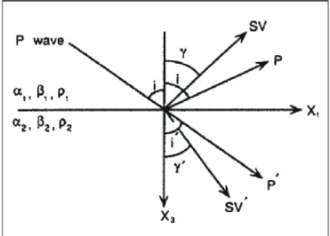
The basic aspect of this method is that as seismic rays cross discontinuities, the energy of the incoming ray is partitioned between reflected and refracted rays (Fig. 15).

Fig. 15- The ray geometry for an incident P wave on a solid-solid interface

and the resulting four derivates: refracted P (P’), reflected P (P), refracted SV (SV’), reflected SV (SV). α, β and ρ represent P wave velocity, S wave velocity and density, respectively.

The geometry of the incident P wave and its derivatives is governed by Snell’s law:

2 1

1 ( )/ ( ')/ ( ')

)

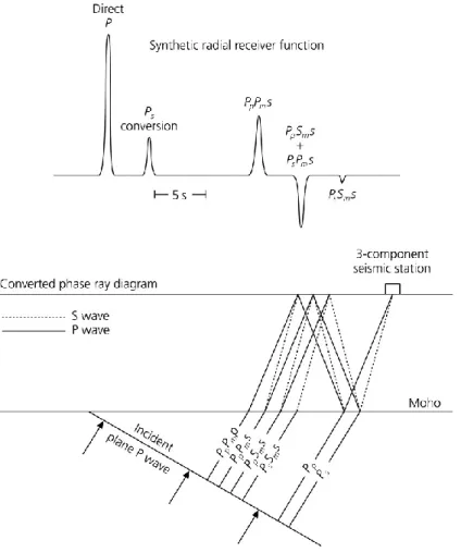
(Sini   Sin   Sin   Sini  (3.1) whereas the amplitudes of the partitioned energy are determined by wave-field theory and represented by reflection and transmission coefficients. Receiver function method is a way to detect, isolate and enhance P-to-SV conversion mode which is produced as teleseismic P waves cross a seismic discontinuity (Fig. 16). Basically, the S waves travel slower than the P waves, so, a direct measure of the depth of the discontinuity is calculated by the time difference in the arrival of the direct P wave and the converted

phase (PS), provided the velocity model is known. In addition to the direct PS converted

phases, the multiples resulting from the discontinuity and free surface, are also seen on the receiver function traces (Figs. 16 and 17).

Fig. 16- Sketch illustrating the major PS converted phases for a layer over a half space

model (bottom). Simplified R-component receiver function corresponding to the model, showing the direct P and PS conversions from the Moho and its multiple (top). (From

Owens et alii, 1987).

The amplitudes of these phases depend on the incidence angle of the impinging P wave, the velocity contrast across the discontinuities and the gradient of the velocity changes. The relative arrival times of the converted phases and multiples depend on the depth of the velocity discontinuities, and the P and S velocity structure between the discontinuity and the surface. Radial RFs primarily provide information about changes in the S-wave velocity in the crust and upper mantle, whereas transverse RFs can provide information on anisotropy and help to identify dipping structures. Simple 3D structures, like dipping interfaces and layers containing hexagonally anisotropic materials, generate periodic patterns in the RF dataset, as a function of BAZ (Levin and Park, 1998). The analysis of such periodicity has been used to infer the presence of

anisotropy in the subsurface (e.g. Bianchi et alii, 2008) or dipping interfaces (e.g. Lucente et alii, 2005). A thorough numerical investigation of effects on receiver functions is described by Cassidy (1992). In this chapter, the methods, which were applied to the data are briefly introduced.

Fig. 17- Moho converted phase PS (Moho at 32 km depth) and

multiples PPPS, PPSS+PSPS on the radial receiver function (bottom)

and their ray paths (top). (From Zhu and Kanamori, 2000).

3.1 Methods

3.1.1 P-to-S receiver function method

The teleseismic P receiver function method has become a popular technique to constrain crustal and upper mantle velocity discontinuities under a seismic station (e.g., Langston, 1977; Owens et alii, 1984; Kind and Vinnik, 1988; Ammon, 1991; Kosarev et alii, 1999; Yuan et alii, 2000). Langston (1977) showed that if the incident P waves arrive at a high angle to the surface, deconvolving the vertical component (on which P wave energy will dominate) from the horizontal radial component (on which the SV waves produced by P-to-S conversions will be recorded) will yield a deconvolved time

series (termed ‘‘receiver function’’ or source equalized trace) on which the major features are S wave arrivals related to P-to-S conversions and reflections in the crust and uppermost mantle beneath the station. P wave energy on the radial component, that is coherent with energy on the vertical component, will be compressed by the deconvolution into a single spike at zero lag time. On the receiver function, all subsequent arrivals after direct P have times calculated relative to the coherence peak, so that peak is commonly referred to as the direct P wave arrival. Because of the large velocity contrast at the crust-mantle boundary, the Moho P-to-S conversion (PS) is often

the largest signal following the direct P. The amplitude, arrival time, and polarity of the locally generated PS phases are sensitive to the S-velocity structure beneath the

recording station. By calculating the time difference in arrival of the converted PS phase

relative to the direct P wave, the depth of the discontinuity can be estimated using a reference velocity model. Preparing the broadband teleseismic data involved a series of quality checks and multiple processing steps in order to isolate, detect and enhance the SV phases hidden in the P coda of teleseismic earthquakes.

Initially each seismogram was rotated from the NEZ (Fig. 18a) to the RTZ (radial/transverse/vertical) (Fig. 18b) coordinate system (using the event’s backazimuth), where R (radial) is calculated along the great circle path between station and event epicenter (positively-directed from event to station), T (transverse) is 90° clockwise from R and Z is vertical (positive up).

The vertical and radial components of motion (Z(t) and R(t), respectively), restituted after the rotation, can be theoretically represented by:

)

(

)

(







s

t

t

z

t

Z

)

(

)

(







t

t

s

r

t

R

where s(t) is the source time function; tk is the arrival time of the kth ray (k = 0 is the

direct P wave); and the sum over n represents a sum over n rays. The amplitude of the

kth arrival of each component is described by zk and rk. The source equalization

procedure of Langston (1979) consists of a simple deconvolution of the vertical component from the radial component of motion:

)

(

)

(

)

(

)

(

)

(

)

(

)

(















Z

R

Z

S

R

S

H





S(ω) is the source spectrum; H(ω) is the Fourier transform of the receiver function, h(t); ω is radial frequency; and





e

r

r

R

)

(







e

z

z

Z

)

(



where zˆ represents the amplitude of the k_k th arrival normalized by the amplitude of the

direct P wave on the vertical component,

z

ˆ



z

/

z

Equation (3.4) is the defining equation for what is frequently called the receiver function.

The receiver function is the time series corresponding to the complex spectral ratio of the radial response to the vertical response. In plane-layered media, for steeply incident plane waves, the receiver function maintains many of the properties of a seismogram. In fact, individual peaks and troughs on the receiver function correspond to individual arrivals on the radial component response to the incident plane wave. Details of the background behind the technique, together with examples, are given by Ammon (1991).

In this study receiver functions were computed using the technique developed by Ligorria and Ammon (1999) through a time-domain deconvolution of the vertical component of a teleseismic waveform from horizontal radial (along path) and tangential components (at 90° to the direction of propagation) of a seismogram for a particular earthquake (Fig. 19). The deconvolution procedure extracts the PS phases (S waves

converted from P at refracting interfaces) with amplitudes of the conversions depending upon the impedance contrast across the interface and the incidence angle. The time domain approach consists of approximating the deconvolution response through a series of Gaussian pulses with adjusted amplitudes and time lags. This technique circumvents stability problems intrinsic to spectral division, leads to a causal response, and generally produces more stable results in the presence of noise (Ligorria and Ammon, 1999).

Fig. 18- Three-component recordings (a) and rotated horizontal components (b) of the

January 12, 2010 (Mw=7.0) seismic event (Haiti region; epicentral distance=77°; backazimuth= 283°). Z, N-S, and E-W represent the recorded vertical, north-south, and east-west components.

Fig. 19- Radial and transverse receiver functions of the January 12, 2010 event shown

in Fig. 18. The naming convention is that the character, ‘R’ or ‘T’, indicates whether this is the P-wave receiver function for the radial or transverse component. For a plane-layered velocity model and no noise, the ‘T’ should be zero. If it is not small this indicates that the original data were bad, or that the structure is not plane-layered and isotropic.

subsurface refractors at different points. Positive amplitudes in the receiver function reveal a velocity increase with depth, while negative amplitudes indicate a velocity decrease with depth. Including multiples paths in the receiver function analysis (it they are properly identified) gives additional information about the exact depth of the Moho discontinuity and the crustal Poisson’s ratio (Zhu and Kanamori, 2000; Yuan et alii, 2002). However, the presence of significant sediments may alter the primary PS

converted phases and make the estimation of the discontinuity depth difficult. An other problem occurs if a dipping interface changes the ray geometry or an anisotropic layer causes shear wave splitting effects. In both cases converted energy is expected to be observed on the T components (Cassidy, 1992; Levin and Park, 1997).

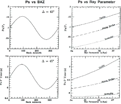
A crucial feature of the receiver function method is that the source equalized traces for events clustered at roughly the same distance and azimuth can be stacked to improve signal-to-noise ratio. However, successful alignment and constructive summation of conversion phases requires that the receiver functions be equalized in terms of their ray parameters. Aligning the move-out corrected receiver functions according to the epicentral distances  (or ray parameters p) not only helps to distinguish the direct conversions, but also allows for enhancement of conversions by constructive summation (stacking) of amplitudes direct conversion whereas the multiples will be substantially suppressed. Move-out correction can also be applied to crustal reverberations. Applying the correction to each multiple and aligning the corrected seismograms by epicentral distance (or ray parameter) leads to straight appearance of the multiples whereas the direct conversions are inclined. After the correction is applied those reverberations which have similar ray parameters appear parallel to each other made. As example, Fig. 20 illustrate the amplitude and arrival-time variations as a function of BAZ and ray parameter (p) for a PS phase generated at an eastward-dipping boundary (strike=N0°E,

dip angle=20°) at 60 km depth (Cassidy, 1992). The most rapid variation in both the amplitude and arrival time of a PS phase generated at a dipping interface occurs along

the strike direction of the boundary. As stated in Cassidy (1992), PS amplitudes always

increase for decreasing  (or increasing ray parameter; see Fig. 20). In contrast, the amplitude of the reverberations may remain constant or even decrease with decreasing  (or increasing ray parameter). This may be useful to discriminate between reverberations and PS conversions. Additionally, reverberations and scattered energy

may be identified by their rapid variations in either amplitude or arrival time over a small range of BAZ or . Thus, for reverberations associated with dipping interfaces,

the variation in the polarity, amplitude, and arrival time as a function of BAZ and , and the large lateral sampling area (relative to PS phases), suggests that it would be

extremely difficult to accurately model such phases. It is obvious that formal inversion techniques, which attempt to match all arrivals in a waveform, must be applied with extreme caution. It would be prudent to begin by forward modeling only for those phases whose amplitude and arrival time variations as a function of both BAZ and  are indicative of PS.

Fig. 20- Amplitude and arrival time variation as a function of backazimuth and

ray parameter (from Cassidy, 1992).

Chen and Liu (2000) investigated the effects of laterally inhomogeneous crustal structure with planar dipping interfaces on the teleseismic receiver function. In case of a single dipping interface the receiver functions vary regularly with azimuths. The regularity of the variations could be summarized into the following main points: (1) The variations of the amplitude and arrival time of each arrival with azimuths have axis clear symmetry for the radial components and asymmetry for the tangential components of the receiver function about the dipping direction of the interface under station. (2) The amplitude ratio of the P wave between the radial and vertical component of the receiver function varies regularly with azimuths. This ratio becomes minimized along the dipping direction and maximized along the inversely dipping direction. A similar

regularity also appears on the tangential component of the receiver function. This phenomenon is caused by the dipping discontinuity under the station. The incident angle at the dipping interface and the emergent angle on the surface are different for different azimuths. (3) On the radial component of the receiver function the phase delay of the PS

converted wave and multiple reflections have the same variation regularity with azimuths. Their phase delays relative to the direct P wave become maximal in the dipping direction and minimal in the inverse dipping direction of the interface. In case of several different dipping interfaces, the wave energy distributions of the receiver function on the vertical, radial and tangential component are changed also, when varying the dipping angle of the interface under the station. These can be summarized into the following main points: the radial and tangential components of the receiver function is no longer symmetric with the azimuth; the arrival time of each phase have no longer consistent regularity of variations with azimuths; there is no incident azimuth, in which the amplitude of the tangential component of the receiver function becomes zero. Therefore, when several different dipping interfaces exist in the receiver structure, the wavefield of the receiver function become much more complicated. Nevertheless, under this complicated case we can find also some of regularities: (1) According to the polarization direction of the first arrival in the tangential component, we can infer the apparent dipping direction of the laterally inhomogeneous structure. So-called apparent dipping direction is not the accurate dipping direction of each interface, but an overall direction of different dipping interfaces. This is only a very rough estimation, but valuable for the further inversion study. (2) Although the amplitudes of the PS converted

waves at each interface are influenced each other, the variations of the PS converted

wave at the second interface are still clear. Therefore, the dipping direction and dipping angle of the second interface can still be estimated.

For theoretical background of the technique used to analyse the waveforms around the world see Kosarev et alii (1987), Kosarev et alii (1993), Kind et alii (1995), Yuan et alii (1997), Sandvol et alii (1998) and Ramesh et alii (2002).

3.1.2 Estimation of crustal thickness and VP/VS ratio

As stated above, receiver functions are created by deconvolving the vertical component from the radial and tangential components of a seismogram for a particular earthquake. Effectively, it turns three different axes of motion from each event into just one seismogram so one can more easily investigate several earthquakes at once. In

particular, using RFs makes it easier to identify the incoming P-wave to S-wave conversions like PS, PPPS, and the combined PPSS+PSPS, all of which involve

conversions of seismic P- and S- waves as they interact with the crust-mantle boundary. By comparing the difference in arrival times between any of these converted phases and the initial P-wave, we can determine the amount of time it takes a certain type of wave to traverse the thickness of the crust. With this information, the velocity and distance travelled can then be determined using a linear relationship. When the linear relationships between all three arrivals for each earthquake are combined, the point of intersection indicates the unique solution to the three lines and it represents the best-fit thickness and wave speed for the crust below that station.

Zhu and Kanamori (2000) proposed a stacking algorithm which sums the amplitudes of receiver functions at the predicted arrival times of the Moho conversion phase and its multiples (PS, PPPS, and PPSS+PSPS) for different crustal thickness H and VP/VS ratios.

Consequently, time domain receiver functions are mapped into H vs. VP/VS domain

without the necessity to read phases.

Using the time difference between the PSMoho phase and the first arrival, the depth to

Moho can be estimated based on the following equation:



 







ps 1 Vs p 1 Vp p

t

H    (3.7)

where H is the depth to Moho, tps is the time delay between the first arrival and the

Moho phase, VS is the S wave velocity, VP is the P wave velocity, and p is the ray

parameter.

However, since the delay time of the S leg is dependent on the shear velocity of the medium, the crustal thickness trades off strongly with the seismic wave velocity (Zhu and Kanamori, 2000). Incorporating multiply reflected phases such as PPPS and

PPSS+PSPS helps to reduce this trade off significantly. The time delays (tPpPs and

tPpSs+PsPs) for PPPS and PPSS+PSPS phases and H can be expressed in the following

equations:



 











To further enhance the signal/noise ratio and reduce lateral variations, multiple receiver functions are stacked in the time domain. Zhu and Kanamori (2000) developed a straightforward approach that adds the amplitudes of the PSMoho and multiples at the

approach essentially transforms the receiver function stacks from the time domain to the H-VP/VS domain. The H-VP/VS domain stacking is defined by:

) ( ) ( ) ( ) / , (H Vp Vs w₁r t_ps w₂r t_PpPs w₃r t_{PpSs PsPs} S    _ (3.10)

where the r(ti) are the receiver function amplitude at the time tPs, tPpPs and tPpSs+PsPs and

w1, w2, and w3 are the weighting factors for each phase that sum to unity.

The function S(H, VP/VS) reaches a maximum when all three phases (PS, PPPS, and

PPSS+PSPS) are stacked coherently (Fig. 21).

Fig. 21- Contributions of PS and its multiples to the stacked

amplitude as a function of crustal thickness (H) and VP/VS ratio.

The obtained H (crustal thickness) and VP/VS ratio are also considered as the best

combination underneath the assumed station if the multiples are clear enough. The main advantage of this technique is that there is no need to pick the arrival times of the Moho or the multiples, making this technique more objective than having to manually identify these various phases. This approach also removes the effects of different ray parameters (p) on the moveout of the listed P-to-S converted phases. When receiver functions contain clear Moho conversions and Moho crustal multiples and spread over broad epicentral distances this method is able to detect the crustal depth as well as average VP/VS ratio with rather high precision. By combining such point data over a seismic

network it is possible to produce maps of crustal thickness and VP/VS ratios which are

Chapter 4

4.1 Data and Methods

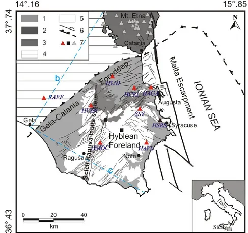
In choosing observations to use for computing receiver functions (RFs), we selected teleseismic events recorded between January 2004 and April 2011 at 8 broadband seismic stations (red triangles in Fig. 22; coordinates and equipments in Table 1 and 2) deployed in southeastern Sicily (Italy), all of which are part of the seismic permanent Network currently operated by the Istituto Nazionale di Geofisica e Vulcanologia (INGV, Osservatorio Etneo, Sezione di Catania). HSRS station (black triangle in Fig. 22), equipped with a short period seismometer, was not used for Moho depth estimation.

Fig. 22- Geological sketch map of southeastern Sicily (modified from Azzaro and

Barbano, 2000). 1=Recent-Quaternary deposits; 2=Late Pleistocene-Holocene Etnean volcanics; 3=Plio-Pleistocene Hyblean volcanics; 4=Appennine-Maghrebian units; 5=Meso-Cenozoic carbonate sediments; 6=normal, strike-slip faults and main thrust fronts; 7=seismic stations (red and black triangles, Sicilian Network; black squares, Italian National Network; gray triangles, Etnean Network). (b) and (c)= traces of the interpretative cross sections shown in Fig. 4.

These stations overlie several interesting geological provinces in the region, covering Recent Quaternary deposits, Plio-Pleistocene Hyblean volcanics, Appennine-Maghrebian units and Meso-Cenozoic carbonate sediments (Fig. 22). The seismic

stations, with an average station spacing of 20-25 km, are set up in Augusta (HAGA), Avola (HAVL), Carlentini (HCRL), Lentini (HLNI), Modica (HMDC), Vizzini (HVZN), Raffadali (RAFF) and Solarino (SSY).

Table 1- Station names and locations

Station Lat.N Long.E Elevation (m) Location Geology

HAGA 37.285 15.155 126 Augusta Plio-Pleistocene Hyblean volcanics HAVL 36.96 15.122 503 Avola Meso-Cenozoic carbonate sediments HCRL 37.283 15.032 190 Carlentini Plio-Pleistocene Hyblean volcanics

HLNI 37.348 14.872 147 Lentini Recent Quaternary deposits HMDC 36.959 14.783 600 Modica Meso-Cenozoic carbonate sediments

HVZN 37.178 14.715 788 Vizzini Plio-Pleistocene Hyblean volcanics RAFF 37.222 14.362 510 Raffadali Appennine-Maghrebian Units

SSY 37.158 15.074 602 Sortino Meso-Cenozoic carbonate sediments

Most stations were active from 2005 (with a few exception of SSY since 2004 and RAFF and HLNI since 2006 and 2009, respectively) and provided good quality recordings of numerous teleseismic earthquakes from around the world. Seismometer Network consists of Nanometrics Trillium 40s velocimetric sensors that measure ground motion over a wide frequency range with a flat response to velocity from 0.025 to 50 Hz; data are digitized at a rate of 100 samples per second by a 24 bit analog-to-digital converter (Table 2).

Table 2- Instrumentations

Station Year Tipology Sensor Sensitivity Bandwitdth Sps Transmission HAGA 2005 Dig. 3C BB T40s 1500 V/m/s 0.025-50 Hz 100 Radio wireless HAVL 2005 Dig. 3C BB T40s 1500 V/m/s 0.025-50 Hz 100 Radio UHF HCRL 2005 Dig. 3C BB T40s 1500 V/m/s 0.025-50 Hz 100 Satellite Transmission VSAT HLNI 2009 Dig. 3C BB T40s 1500 V/m/s 0.025-50 Hz 100 Satellite Transmission VSAT HMDC 2005 Dig. 3C BB T40s 1500 V/m/s 0.025-50 Hz 100 Radio UHF HVZN 2005 Dig. 3C BB T40s 1500 V/m/s 0.025-50 Hz 100 Satellite Transmission VSAT RAFF 2006 Dig. 3C BB T40s 1500 V/m/s 0.025-50 Hz 100 Satellite Transmission VSAT SSY 2004 Dig. 3C BB T40s 1500 V/m/s 0.025-50 Hz 100 Satellite Transmission VSAT

Dataset, selected by searching the IRIS-DMC catalogue, includes 335 teleseisms (see Appendix A) with moment magnitude (Mw) 6.0 and larger and epicentral distance (great circle arc between source and station) between 30° and 95°. The distributions, according to their epicentral distance, are given in Fig. 23 and geographic locations are given in Fig. 24.

Fig. 23- Distribution of events according to their epicentral distance.

Fig. 24- Stereographic projection of the Earth centred on SSY

station showing the locations of teleseismic events collected between January 2004 and April 2011 (Mw greater than or equal 6.0 occurring between 30 and 95 degrees).

The magnitude has to be adequately high in order to ensure a large signal to noise ratio, while the spatial constraints on this search are to ensure a steep incidence angle on

the incoming ray path, which maximize incoming wave energy, allow for the transmission of S-waves, and minimize disruptions due to lateral inconsistencies and vertical velocity contrasts (Hobbs and Darbyshire, 2012). The application of these selection criteria resulted in the acquisition of a adequate number of recordings for each station.

After a first visual inspection, through which we excluded seismic waveforms with a low signal to noise ratio, we obtained a dataset of about 1600 three-component records, with a minimum of 117 (HMDC) and a maximum of 297 (RAFF) three-component records for each station.

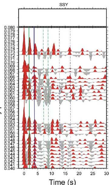
Receiver functions were computed using the technique developed by Ligorria and Ammon (1999) through a time-domain deconvolution. To improve the signal-to-noise ratio, receiver functions obtained for individual earthquakes were binned, moveout corrected and subsequently stacked. The method has been described in detail in Chapter 3. RFs were derived using 120 s time windows (starting 20 s before the P arrival; 20 s pre-event and 100 s post-event). RFs have been band-passed using a Gaussian filter to smooth high frequency (Ligorria and Ammon, 1999). Four different Gaussian filters, with parameter a=0.5, a=1, a=2.5 and a=5 which exclude frequencies higher than about 0.24, 0.5, 1.24 and 2.5 Hz, respectively, have been used. This permitted to subsequently examine frequency dependences in the observed RFs (Owens and Zandt, 1985; Cassidy, 1992). In the following, the estimated RFs described have frequency cut-offs of 1.24 Hz, unless specifically mentioned otherwise. This frequency band is adequate for crust-scale receiver function analysis. We collected an average of 66 RFs with a high signal-to-noise ratio for each station (receiver functions have been calculated only for earthquakes with a signal-to-noise ratio larger that 2). A better signal-to-noise ratio was achieved by stacking the RFs coming from the same backazimuth direction (Park et alii, 2004). Bins are computed every 10° in BAZ using a 50% overlapping scheme, so each bin shares its events with the two adjacent bins. The spread of event epicentral distance for any one bin was small. In the following, the radial (R) and transverse (T) components of all the receiver functions are sorted by backazimuth and corrected by Ps moveout, along with the backazimuth of each trace (named BAZ). The term ‘backazimuth’ is used to refer to the direction from the station towards the earthquake epicentre, measured clockwise from north. The aim of the moveout correction is to equalize differences in ray parameters in the phase arrival times to allow for direct comparison of receiver functions for earthquakes from different distances. We used a

ray parameter of 0.052 s/km as reference. This representation gives information about laterally varying structures and the complexity of the discontinuities (i.e., presence of dipping, scattering and/or anisotropy). Positive amplitudes are shaded in red and indicate an increasing velocity with depth, whereas negative amplitudes (shaded in gray) show velocity decreasing downwards. The P onset is fixed to be as zero time. The sum traces, in the upper panels, present the stacked P receiver function for each station. Stacking all RF from different BAZ directions suppresses features in the dataset which are generated from local heterogeneities and highlights the bulk 1D structure under the station. The R receiver functions, sorted by the ray parameter, are also shown. We stacked them into bins of 0.002 s/km, moving the bin every 0.001 s/km. This representation helps us to distinguish between converted and multiple phases (Cassidy, 1992). The converted phases exhibit a positive moveout and an increase in amplitude with respect to the direct P with increasing ray parameter, while the multiples present a negative moveout and a constant amplitude with the ray parameter (Cassidy, 1992). It should be pointed out, however, that multiples, conversion interference and data noise also affect pulse amplitudes in complex ways, therefore an error could be introduced into the resulting images.

In principle, we used the simplest and straightforward approach that consists in identifying the PS phase converted at the crust-mantle boundary and computed crustal

thickness from the PSMoho-P time delay, given a bulk crustal velocity. The identification

of the Moho PS conversion is made mainly with two criteria: (1) its expected delay of

~4-5 s with respect to the direct arrival for the Hyblean Foreland where the crust is estimated to be on average about ~30-40 km thick and (2) its moveout with ray parameter (or epicentral distance).

Then, we examined the first seconds of RFs, since shallow crustal structures always strongly influence the first seconds, and dipping high-velocity contrast interfaces and/or anisotropic layers with tilted symmetry axis produce characteristic BAZ patterns of direct P waves and PS converted phases (Levin and Park, 1997). Therefore, looking at

the azimuthal variation in the tangential receiver functions, we looked for polarity flips of the converted phases that are consistent with anisotropic or dipping-interface effects. Several workers have investigated the effects of anisotropy and layer dip on teleseismic wave propagation (Langston, 1977; Cassidy, 1992; Levin and Park, 1998; Savage, 1998; Piana Agostinetti et alii, 2008). Both factors lead to backazimuthal variations in the impulse response, involving traveltime and amplitude, as well as the rotation of P-SV