ALMA MATER STUDIORUM – UNIVERSITÀ DI BOLOGNA
SCUOLA DI INGEGNERIA E ARCHITETTURA
DOTTORATO DI RICERCA IN
MECCANICA E SCIENZE AVANZATE DELL'INGEGNERIA
Ciclo XXX
Settore Concorsuale di afferenza: 09/C2 Settore Scientifico disciplinare: ING-IND/10
TITOLO TESI
:
Finite element analysis of heat transfer in
double U-tube borehole heat exchangers
Presentata da
: Aminhossein Jahanbin
Coordinatore Dottorato
:
Relatore
:
Prof. Marco Carricato
Prof. Enzo Zanchini
I
Abstract
The present Ph.D. dissertation deals with the finite element analysis of the heat transfer processes in double U-tube Borehole Heat Exchangers, called BHEs. As the main outline of this study, it can be pointed out to the analysis of the working fluid temperature distribution, proposing correlations to determine the mean fluid temperature, and the analysis of the thermal resistance and effects of the temperature distribution on it, for double U-tube BHEs. In the evaluation of thermal response tests (TRTs), in the design of the BHE fields, and in the dynamic simulation of ground-coupled heat pumps (GCHPs), the mean temperature Tm of the working fluid
in a BHE, is usually approximated by the arithmetic mean of inlet and outlet temperatures. In TRTs, this approximation causes an overestimation of the thermal resistance of the heat exchanger. In the dynamic simulation of GCHPs, this approximation introduces an error in the evaluation of the outlet temperature from the ground heat exchangers. In the present thesis, by means of 3D finite element simulations, firstly, the analysis of the fluid temperature distribution is carried out, then, correlations are proposed to determine the mean fluid temperature, for double U-tube BHEs. Tables of a dimensionless coefficient are provided that allows an immediate evaluation of Tm in any working condition, with reference to double
U-BHEs with a typical geometry. These tables allow a more accurate estimation of the borehole thermal resistance by TRTs and a more accurate evaluation of the outlet temperature in dynamic simulations of GCHP systems. Criteria for the extension of the results to other geometries are also provided. In addition, the effects of the surface temperature distribution on the thermal resistance of a double U-tube BHE are investigated. It is shown that the thermal resistance of a BHE cross section (2D) is not influenced by the bulk-temperature difference between pairs of tubes, but is influenced by the thermal conductivity of the ground when the shank spacing is high. Then it is shown that, if the real mean values of the bulk fluid temperature and of the BHE external surface are considered, the 3D thermal resistance of the BHE coincides with the thermal resistance of a BHE cross section, provided that the latter is invariant along the BHE. Eventually, the difference between the BHE thermal resistance (2D or 3D) and the effective BHE thermal resistance, defined by replacing the real mean temperature of the fluid with the average of inlet and outlet temperatures, is evaluated in relevant cases.
III
Sommario
La presente Tesi di Dottorato tratta dell’analisi agli elementi finite dei processi di trasmissione del calore in scambiatori verticali con il terreno detti “Borehole Heat Exchangers”, BHEs, con riferimento a BHEs a doppio tubo a U. Lo studio è incentrato sull’analisi della distribuzione della temperatura del fluido operatore e degli effetti che questa distribuzione ha sulla resistenza termica dello scambiatore. I risultati principali sono costituiti da correlazioni che consentono di determinare la temperatura media del fluido nello scambiatore e dallo studio degli effetti della distribuzione di temperatura sulla resistenza termica dello scambiatore. Nella valutazione di Test di Risposta Termica (TRTs), per il progetto di campi di BHEs, e nella simulazione dinamica di pompe di calore accoppiate al terreno (Ground-Coupled Heat Pumps, GCHPs), la temperatura media Tm del fluido operatore in un
BHE è abitualmente approssimata dalla media aritmetica della temperatura in ingresso e di quella in uscita del fluido. Nei TRT, questa approssimazione causa una sovrastima della resistenza termica dello scambiatore. Nella simulazione dinamica delle GCHPs, questa approssimazione introduce un errore nel calcolo della temperatura in uscita dallo scambiatore di calore. In questa Tesi, la distribuzione di temperatura del fluido nello scambiatore viene studiata mediante accurate simulazioni 3D agli elementi finiti, quindi vengono proposte semplici correlazioni adimensionali che consentono di determinare la temperatura media Tm del fluido in
qualsiasi condizione operativa, date le temperature in entrata e in uscita e la portata in volume del fluido e la conducibilità termica della malta sigillante. Le correlazioni si riferiscono a BHEs a doppio tubo a U con una geometria tipica. Sono forniti anche criteri per l’estensione dei risultati ad altre geometrie. Vengono inoltre analizzati gli effetti della distribuzione di temperatura superficiale dello scambiatore sulla resistenza termica dello stesso. Si mostra che la resistenza termica 2D di una sezione trasversale non è influenzata dalla differenza della temperatura di bulk fra coppie di tubi, ma è influenzata dalla conducibilità termica del terreno circostante se l’interasse fra i tubi è elevato. Si mostra anche che, se vengono considerati i veri valori della temperatura media di bulk del fluido e della temperatura alla superficie esterna dello scambiatore, la resistenza termica 3D dello scambiatore coincide con quella 2D di una sezione trasversale, a condizione che questa possa essere considerata invariante lungo lo scambiatore. Infine, viene calcolata in alcuni casi rilevanti la differenza fra la vera resistenza termica dello scambiatore (2D o 3D) e la resistenza termica detta “effettiva”, che si ottiene approssimando la temperatura media di bulk del fluido con la media aritmetica delle temperature in entrata e in uscita.
V
I would like to express my sincere gratitude to my supervisor Professor Enzo Zanchini for his support and priceless guidance throughout my doctoral course.
VII
IX Abstract . . . I Contents . . . . . . IX List of figures . . . XI List of tables . . . XV Nomenclature . . . . XVII 1 Preface . . . 1
2 An introduction on Ground-Coupled Heat Pump (GCHP) systems . . . 7
2.1 Ground-Source Heat Pumps (GSHPs) and their categories . . . 11
2.2 Ground-Coupled Heat Pumps (GCHPs) . . . 13
2.3 BHE field design methods . . . 15
2.3.1 Analytical models . . . 16
2.3.2 Numerical models . . . 22
2.3.3 Analytical models vs. numerical models . . . 24
2.4 Fluid-to-ground thermal resistance . . . 24
2.5 Hybrid GCHP systems . . . 26
3 Heat transfer analysis of U-tube BHEs . . . 29
3.1 Heat transfer models for the BHE thermal resistance . . .
34
3.2 Estimation of the BHE thermal resistance . . . 40
3.3 Convective heat transfer inside tubes . . . 42
4 Numerical method . . . 49
4.1 Finite element analysis . . . 51
4.2 Numerical model . . . 53
X
6 Correlations to determine the mean fluid temperature . . .
75
6.1 Model validation . . . 80
6.2 Results for quasi-stationary regime . . . 83
6.3 Results for the first two hours . . . 88
6.4 Possible applications . . . 91
7 Effects of the temperature distribution on the thermal resistance . . . .
95
7.1 Thermal resistance of the cross section of a double U-tube BHE . . . 99
7.2 Relations between Rb,eff, Rb,3D and Rb,2D for double U-tube BHEs . . . . 104
7.2.1 A theorem on the relation between Rb,3D and Rb,2D . . . 105
7.2.2 Results of computational analysis . . . 106
8 Conclusions & prospective
. . . 113 References . . . 119
XI
2.1 U.S. annual primary energy consumption by source from 1950 to 2015, data according to EIA [1]. 10
2.2 Europe final energy consumption percentage by sector in 2015, data according to Eurostat [5]. 11
2.3 Iceland's Nesjavellir geothermal power station. Geothermal plants account for more than 25 percent of the electricity produced in Iceland. Photo: Gretar Ívarsson [8]. .. . .
12
2.4 Schematic of a GSHP system in heating/cooling mode, reported by EPA [12]. . . . . . . 13
2.5 The installed capacity and annual utilization of geothermal heat pumps from 1995 to 2015 [15]. 14
2.6 A vertical closed-loop GCHP system [18]. . . . 15
2.7 Fourier / G-factor graph for ground thermal resistance [9]. . . . 20
2.8 Earth Energy Designer - EED [40]. . . . 22
2.9 A BHE cross section. . . . 25
2.10 Thermal resistive network for a single U-tube BHE. . . . 26
2.11 Schematic diagram of a HGCHP system with solar collector, presented in reference [44]. . . . 27
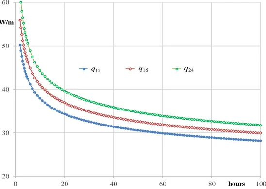
3.1 Temperature distribution in a double U-tube BHE and the surrounding ground. . . . 33
3.2 Cross section of a double U-tube BHE.
. . . 34
4.1 COMSOL Multiphysics desktop environment. . . . 53
4.2 Sketch of the BHE cross section considered. . . . 54
4.3 3D mesh of the BHE and the surrounding ground. . . . 56
4.4 Mesh of the BHE for a 2D simulation case. . . . 60
4.5 3D mesh of the BHE and the surrounding ground. . . . 60
4.6 Convergence plot for a time-dependent solver. . . . 61
4.7 Plot of fluid temperature distribution along the vertical coordinate z, compared with that yielded by the method of Zeng et al. [70], for kgt = 1.6 W/(mK) and volume flow rate 12 L/min. 62 4.8 Mesh independence check for modified code (Code II), plots of Tave - Tm versus time. . . . 63
5.1 Illustration of the BHE cross section. . . . 68
5.2 Power per unit length extracted from the ground: water with inlet temperature 4 °C. . . . 69
5.3 Power per unit length extracted from the ground: water-glycol with inlet temperature -2 °C. . . .
70
XII
5.6 Fluid temperature distribution versus height z (m) for the volume flow rate 24 L/min:
water with inlet temperature 4 °C. . . . . . .
72
6.1 Enthalpy balance of the fluid heating tank. . . . 79 6.2 Time evolution of Tave - Tm obtained numerically and through the analytical model
by Zeng et al. [70], for kgt = 1.6 W/(mK), kg = 1.8 W/(mK), flow rate 12 L/min. . . . 81
6.3 Time evolution of Tave - Tm obtained numerically and through the analytical model
by Zeng et al. [70], for kgt = 1.6 W/(mK), kg = 1.8 W/(mK), flow rate 24 L/min. . . . 82
6.4 Comparison between the experimental time evolution of Tin_exp and that obtained through
equation (6.5), denoted by Tin_num, for a TRT performed at Fiesso d’Artico (Venice) [96]. . . . 83
6.5 Time evolution of for kgt = 1.6 W/(mK), kg = 1.8 W/(mK), flow rates 12 and 24 L/min. . . . 84
6.6 Linear interpolations of Tave - Tm as a function of
TinTout
V, for kgt = 0.9, 1.2, 1.6 W/(mK). 856.7 Effects of different values of kg, namely 1.4 and 2.2 W/(mK), for kgt = 0.9 W/(mK). . . 86
6.8 Effects of different values of kg, namely 1.4 and 2.2 W/(mK), for kgt = 1.6 W/(mK). . . . 86 6.9 Effects of different values of the BHE diameter, for kgt = 1.2 W/(mK) and kg = 1.8 W/(mK). . . . 87
6.10 Effects of different working conditions, for kgt = 1.6 W/(mK) and kg = 1.8 W/(mK). . . 87
6.11 Plots of versus t*, for kgt = 0.9 and kgt = 1.6 W/(mK), with flow rate 12 L/min,
in the range 1 120 t* 0.6.
. . . 89
6.12 Plots of versus t , for k* gt = 0.9 and kgt = 1.6 W/(mK), with flow rate 18 L/min,
in the range *
1 120 t 0.6. . . . 89 6.13 Plots of mean1 versus V V0, for kgt = 0.9, 1.2 and 1.6 W/(mK). . . 90 6.14 Plots of versus t for TRTs with k*
gt = 1.6 and kg = 1.8 W/(mK): flow rate 12 L/min,
power 50 W/m, *
8 120t 1; flow rate 24 L/min, power 80 W/m, *
4 120t 1. . . . .
91
7.1 Illustration of the definition of thermal resistance: the lateral surfaces are tangent to the
heat flux density vector q. . . . 99 7.2 Cross section of the BHE considered, with shank spacing 85 mm (left) and 120 mm (right). . . . 100
XIII
kg = 1.4 W/(mK), scheme 4. . . . 104
7.4 Plot of Tf versus the vertical coordinate z, compared with that yielded by the method of
Zeng et al. [70], Tf_Z, for kgt = 1.6 W/(mK) and volume flow rate 12 L/min. . . . 106 7.5 Plot of Tf,in - Tf,out versus time, compared with that yielded by the method of Zeng et al. [70],
(Tf,in - Tf,out)_Z, for kgt = 0.9 W/(mK) and volume flow rate 12 L/min. . . . 107
7.6 Plot of Tf,in - Tf,out versus time, compared with that yielded by the method of Zeng et al. [70],
(Tf,in - Tf,out)_Z, for kgt = 0.9 W/(mK) and volume flow rate 24 L/min. . . . 108
7.7 Plot of Tf,in - Tf,out versus time, compared with that yielded by the method of Zeng et al. [70],
(Tf,in - Tf,out)_Z, for kgt = 1.6 W/(mK) and volume flow rate 12 L/min. . . . 109
7.8 Plot of Tf,in - Tf,out versus time, compared with that yielded by the method of Zeng et al. [70],
(Tf,in - Tf,out)_Z, for kgt = 1.6 W/(mK) and volume flow rate 24 L/min. . . . 109 7.9 Plots of Rb,eff and of Rb,3D versus time, compared with the steady-state value (Rb,eff)_Z
yielded by the method of Zeng et al. [70], for kgt = 0.9 W/(mK) and volume flow rate 12 L/min.
110
7.10 Plots of Rb,eff and of Rb,3D versus time, compared with the steady-state value (Rb,eff)_Z
XV
3.1 Shape factors for three different patterns of the shank spacing [66]. . . . 35
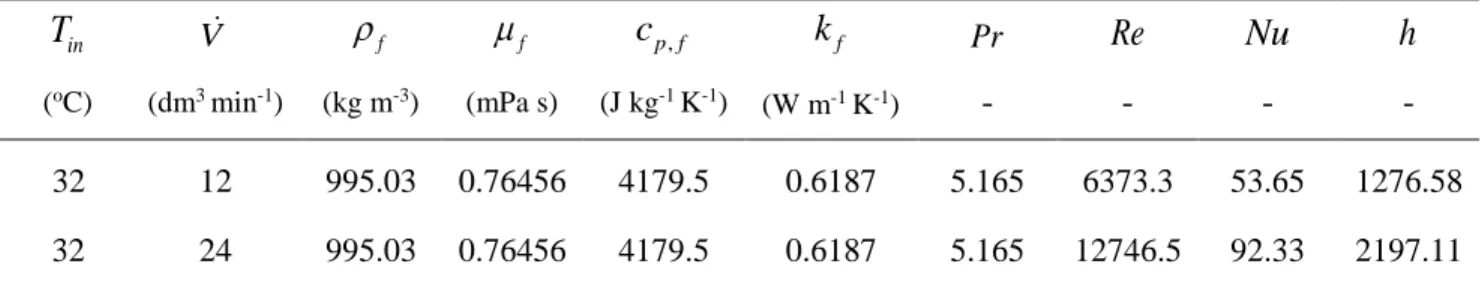
3.2 Thermophysical properties and fluid flow characteristics in a simulation performed in the present study. . . . 46
4.1 The thermophysical properties adopted in Code I, taken from reference [91]. . . 56
4.2 Values of water thermophysical properties and flow characteristics [91]. . . . 57
4.3 Mesh independence check for the first code employed (Code I). . . . 62
4.4 Mesh independence check for modified code (Code II). . . . 63
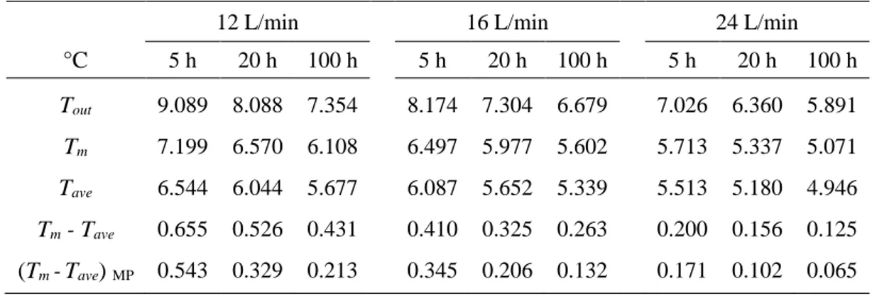
5.1 Values of Tout , Tm , Tave , Tm - Tave and (Tm - Tave) MP for water, with Tin = 4 °C.
. . . 70
5.2 Values of Tout , Tm , Tave , Tm - Tave and (Tm - Tave) MP for water-glycol, with Tin = -2 °C. . . . 71
6.1 Values of
and of the coefficients a and b of equation (6.16). . . . 886.2 Values of mean1 as a function of kgt and of V V0. . . . 90
7.1 Values of the 2D thermal resistance for shank spacing 85 mm (figure 7.1, left), obtained by different calculation schemes. . . . 102
7.2 Values of the 2D thermal resistance for shank spacing 120 mm (figure 7.1, right), obtained by schemes 1, 3, 5 and equation (7.8). . . . 103
7.3 Values of Tf,in - Tf,out after 100 hours of operation, compared with those yielded by the method of Zeng et al. [70].
. . . 108
7.4 Values of (Rb,eff)_Z, asymptotic values of Rb,eff and Rb,3D, and steady values of Rb,2D. . . . 111
XVII
a, b dimensionless coefficients A pipe cross section area (m2)
Cw heat capacity at constant pressure of a fluid tank (J K–1)
cp specific heat capacity at constant pressure (J kg–1 K–1)
d distance between centers of opposite tubes (shank spacing) (m)
D diameter (m)
erfc complementary error function f dimensionless parameter fr friction factor
Fsc short circuiting heat loss factor
Fo Fourier number g g-function G G factor
g gravity (m s-2)
Gr Grashof number
h heat transfer coefficient (W m–2 K–1) Jn Bessel function of first kind with order n
k thermal conductivity (W m–1 K–1)
k
= k/100, reduced thermal conductivity (W m–1 K–1)L length (m)
m mass flow rate (kg s–1) n number of pipes Nu Nusselt number p real coefficient PLF part-load factor Pr Prandtl number
q flux density vector (W)
XVIII
a
q heat flux per unit area (W m-2) Q heat source/sink (W)
r radial coordinate, radius (m) R BHE thermal resistance (mKW–1)
Rb,2D thermal resistance of a BHE cross section (mKW–1)
Rb,3D 3D BHE thermal resistance (mKW–1)
Rb,eff effective BHE thermal resistance (mKW–1)
R11 thermal resistances between the fluid and the BHE external surface (mKW–1)
R12 thermal resistances between two adjoining tubes (mKW–1)
R13 thermal resistances between two opposite tubes (mKW–1)
Re Reynolds number S1, S2 Boundary surfaces (m2) t time (s) T temperature (K) u velocity field (m s-1) u velocity (m s-1)
u = u/10, reduced fluid velocity (m s-1) V volume (m3)
V volume flow rate (m3 s-1)
W system power input (W) x, y horizontal coordinates (m)
Yn Bessel function of second kind with order n
z vertical coordinate (m)
z = z/10, reduced vertical coordinate (m)
Z = z/L, dimensionless vertical coordinate
Greek symbols
α thermal diffusivity (m2 s–1)
XIX non-dimensional geometrical parameter
dynamic viscosity (Pa s) ν kinematic viscosity (m2 s-1)
density (kg m–3)
(c) specific heat capacity per unit volume (J m–3 K–1) σ dimensionless parameter 1, 12 dimensionless parameters φ dimensionless parameter dimensionless parameter Subscripts / Superscripts * dimensionless quantity 0 reference value
12 of volume flow rate 12 L/min 16 of volume flow rate 16 L/min 24 of volume flow rate 24 L/min
∞ quasi-stationary regime / asymptotic value anl annual
ave average
b of BHE
c cooling
cond conductive heat transfer conv convective heat transfer d of fluid going down
Darcy refers to Darcy friction factor des refers to building design dly daily
e refers to external radius/diameter of pipe eff effective
XX
g of ground
g0 refers to undisturbed ground
gt of grout
h heating
hyd hydraulic
i refers to internal radius/diameter of pipe i-th i th
in refers to inlet
l refers to laminar flow regime lc refers to laminar flow at Re=2100
m mean value
mean1 mean value during the first hour mly monthly
MP obtained by the method of Marcotte and Pasquier [66] num numerical
out refers to outlet
p of pipe, of polyethylene
pen refers to temperature penalty for interference of adjacent bores pf at the surface between pipe and fluid
ref reference
s of BHE external surface t refers to turbulent flow regime tot total value
tr refers to transient flow regime
th thermal
u of fluid going up
1
Chapter 1
3
1
Preface
Adoption of renewable energy sources, and particularly geothermal energy, is an optimal way to shift from fossil-based development to sustainable development. Ground-Source Heat Pump (GSHP) systems are becoming increasingly a rather widely used technology for building heating, cooling, and also for Domestic Hot Water (DHW) production while incurring low maintenance cost. Many reports have shown that GSHP systems are more economically advantageous and eco-friendly than the traditional heating systems. In particular, Ground-Coupled Heat Pumps (GCHPs) appear as the most promising kind of GSHPs for the future developments, due to their applicability and possibility of installation in almost every ground. The most diffuse GCHP systems utilize vertical ground heat exchangers, called Borehole Heat Exchangers (BHEs). A vertical BHE is typically composed of pipes in high-density polyethylene, inserted in a drilled hole which is sealed with grouting materials. The pipe configurations within the borehole may be a single U-tube, double U-tube or coaxial arrangement. The length of the BHE is usually between 50 and 150 m, and the most common diameter is about 15 cm. The cases under study in this thesis are double U-tube BHEs commonly employed in Northern Italy.
The design of a BHE field requires the knowledge of the undisturbed ground temperature, of the thermal conductivity and thermal diffusivity of the ground, as well as of the thermal resistance per unit length of the BHE. These parameters can be determined through a Thermal Response Test (TRT) which is performed by a procedure recommended by ASHRAE (the American Society of Heating, Refrigerating and Air-conditioning Engineers) and usually evaluated by the infinite line-source approximation model. In this evaluation method, the mean fluid temperature is approximated by the arithmetic mean of inlet and outlet temperatures, that we call it average temperature. Some authors pointed out that, on account of the thermal short-circuiting between the descending and the ascending flow, a significant difference between the real mean fluid
4
temperature and that obtained by average of inlet and outlet temperatures can occur. This error yields an overestimation of the BHE thermal resistance that is determined by the infinite line-source evaluation of a TRT. Hence, a correct estimation of the mean fluid temperature plays an important role in the evaluation of the TRT.
The hourly simulation of the GCHP systems is another technical problem in which the knowledge of the relation between inlet, outlet and mean fluid temperature is useful. In the dynamic simulation of GCHPs, an error in the estimation of the mean fluid temperature yields an error in the evaluation of the outlet temperature from ground heat exchangers, and as a consequence, of the heat pump efficiency. Therefore, precise correlations to evaluate the mean fluid temperature would allow a more accurate estimation of the BHE thermal resistance by a TRT and of the outlet fluid temperature in the dynamic simulation of GCHP systems.
The scope of this study is to analyze the thermal characteristics of double U-tube vertical ground heat exchangers by means of finite element simulations. In particular, the main objectives of this thesis can be classified as:
Analysis of the fluid temperature distribution over the length of tubes Proposing correlations to determine the mean fluid temperature
Evaluation of the effects of the temperature distribution on the BHE thermal resistance A brief description of the chapters is presented in the following.
After preface, the second chapter of this thesis presents an introduction on Ground-Coupled Heat Pump (GCHP) systems. A review on employing the renewable energy sources, particularly geothermal energy, is carried out and the Ground-Source Heat Pump (GSHP) systems and their categories are studied. In addition, a classification of the various methods for BHE field design is provided and differences between these methods are stressed, where it is relevant.
Heat transfer processes in U-tube BHEs are investigated in chapter 3. Internal heat transfer mechanism, theories and different definitions for the thermal resistance of U-tube BHEs, and convective heat transfer inside the tubes are presented.
The numerical approaches employed in this study are presented in chapter 4. This chapter contains a review on finite element analysis method and explanations regarding the software utilized, mathematical modeling, model validation, and boundary and working conditions. Finally, it renders some explanatory notes on the program solver, convergence results, meshes employed and grid independence.
In chapter 5, the fluid temperature distribution is analyzed by means of the finite element method, for a typical double U-tube BHE, under various unsteady working conditions. The difference between the mean fluid temperature and the arithmetic mean of inlet and outlet temperatures is determined and validated by an analytical method.
New correlations to determine the mean fluid temperature of double U-tube BHE are proposed in chapter 6. By means of 3D simulations, tables of a dimensionless coefficient are provided which allow an immediate evaluation of the mean fluid temperature of BHEs in any
5
working condition, including TRTs. In addition, the applicability of the correlations to different BHE geometries are investigated.
Chapter 7 is devoted to the study of the thermal resistance of double U-tube BHEs and of the effects of temperature distribution on it. In this chapter, different definitions of the BHE thermal resistance, presented in chapter 3, are considered. Furthermore, the accuracy of approximate analytical models to estimate the thermal resistance is checked by comparison with the results of various 2D and 3D finite element simulations. The parameters that may affect the thermal resistance of double U-tube BHEs are evidenced.
Finally, chapter 8 reports the conclusion of the present thesis and points out potential opportunities for future studies.
7
Chapter 2
An introduction on Ground-Coupled
Heat Pump (GCHP) systems
9
2
An introduction on
Ground-Coupled Heat Pump (GCHP) systems
Due to the industrial development, improved living standards, urbanization, and population growth, the rate of world energy demand is still rising. As a consequence, the use of primary energy is increasing and fossil fuels, particularly conventional fossil fuels (oil, coal and natural gas), play a key-role as a world primary energy source. Based on EIA (US Energy Information Administration) data [1], the world annual primary energy consumption in 2015 was more than 571 EJ, which was more than 49% higher than of that in 1995. In particular, almost 86% of the world total primary energy use in 2015 was due to the conventional fossil-based energy sources. For the United States, consumption of conventional fossil fuels was 81% of the total primary energy consumption in 2015. The United States annual primary energy consumption by source, from 1950 to 2015, is illustrated in figure 2.1.
However, meeting the today’s ever increasing demand for fossil fuels has become a cause of concern due to the adverse effects of the use of fossil fuels on our planet. Reducing emission of greenhouse gases (GHG), mainly CO2, causing the climate change called global warming, and preserving the fossil fuel sources are important challenges to be faced. Such challenges can be met via reducing the consumption of fossil fuels and exploiting alternative green energy sources.
Incremental adoption of the renewable energy sources is considered as an optimal way to shift from fossil-based development to sustainable development. Consequently, the utilization of renewable energy sources is becoming widely popular and all around the world, governments attempt to move towards a sustainable development. According to the world energy assessment
10
reported by United Nation (UN) in 2000 [2], at the turn of the century, renewable sources supplied almost 14% of the total world energy demand and is expected to reach 50% by 2040 [3,4].
Figure 2.1. U.S. annual primary energy consumption by source from 1950 to 2015, data according to EIA [1].
During the last decade, the European Union energy strategy has been based on the utilization of the renewable energy sources. Based on Eurostat (European Commission portal for statistics) [5], the share of renewable energy in gross final energy consumption, in 28 countries of European Union, has increased more than 77% from 2004 to 2014.
Figure 2.2 shows Europe’s final energy consumption by sector in 2015 [5]. It can be seen that after transport sector, residential consumption and industry were highest final energy consumer sectors in European Union in 2015. The figure shows that the residential sector and the service sector, both based on building operation, reach together about 40% of the total energy consumption. Hence, one important step towards the reduction of the use of fossil-based energy in Europe is to employ renewable energy sources for building operation, according to the Directive of the European Parliament [6].
Geothermal energy refers to the thermal energy projecting from the earth’s crust (thermal energy in rock and fluid), which flows to the surface by conductive heat transfer mechanism and also by convection in regions where geological condition allows. It is believed that the earth would have cooled and become solid from a completely molten state thousands years ago and
0 20 40 60 80 100 EJ year
Total Fossil Feuls Consumption Total Renewable Energy Consumption Nuclear Electric Power Consumption
11
observations have been shown that the ultimate source of geothermal energy is radioactive decay within the earth [7].
Geothermal energy is not only considered as a renewable energy, but it is also considered as a sustainable source of energy. Since any projected heat extraction from the ground is negligible compared to the internal earth’s heat source, geothermal energy can be considered as a renewable energy. Thanks to the power of the earth’s ecosystem, employing current sources of geothermal energy will not endanger the future generations’ resources. Therefore, geothermal energy can be classified as a sustainable energy. Furthermore, geothermal energy is fully potential to mitigate the global warming problem because of its insignificant emissions.
Geothermal plants account for more than one-fourth of the electricity produced in Iceland. Figure 2.3 illustrates Iceland's Nesjavellir geothermal power station [8].
Since geothermal energy is categorized as a renewable energy source, by a Directive of the European Parliament [6], employing Ground-Source Heat Pumps (GSHPs) would be an appropriate solution to meet the European Union energy strategy. GSHPs can be used in buildings in order to supply heating, cooling (air conditioning), and Domestic Hot Water (DHW).
Figure 2.2. Europe final energy consumption percentage by sector in 2015, data according to Eurostat [5].
2.1 Ground-Source Heat Pumps (GSHPs) and their categories
In general, systems employing geothermal energy can be classified in three main types: Direct use and district heating systems, Electricity generation power plants and Geothermal heat pumps. GSHPs, referred to as geothermal heat pumps, were originally developed in the residential arena
25.3 2.2 33.1 0.4 25.3 13.6
Final Energy Consumption by Sector
12
and now are widely applied in the commercial sector [9]. While the temperatures above the ground surface change depending on time of day and season, temperatures more than 3m below the earth's surface are consistently between 10 oC and 15.6 oC. Thus, it can be said that the ground temperatures, for most areas, are usually warmer than the air in winter and cooler than the air in summer. Geothermal heat pumps use the ground’s near-constant temperatures along seasons for both heating and cooling in buildings. Namely, the heat from the ground is transferred into the building during the winter, and the process is reversed in the summer [10]. Employing the earth instead of ambient air provides a lower-temperature sink for cooling and a higher-temperature source for heating with smaller temperature fluctuations, thereby yielding higher efficiency for the heat pump [11]. Figure 2.4 illustrates the schematic of a GSHP system in heating/cooling mode [12].
Figure 2.3. Iceland's Nesjavellir geothermal power station. Geothermal plants account for more than 25 percent of the electricity produced in Iceland. Photo: Gretar Ívarsson [8].
Thanks to their features, GSHPs have been recognized as being cost effective, energy efficient and environmentally friendly systems. GSHPs have the lowest CO2 emissions and the lowest overall environmental costs among of all technologies analyzed, based on the US Environmental Protection Agency data [13]. In addition, these energy efficient systems incur low maintenance costs to heat and cool buildings [14]. As a consequence, the installation rate of GSHPs for heating and cooling in buildings is increasing in several countries.
According to Lund and Boyd [15], the worldwide installed capacity of GSHPs has increased from 1.854 GW to 50.258 GW, from 1995 to 2015 (figure 2.5). Moreover, GSHPs are the systems with the largest share of geothermal energy use and installed capacity worldwide in 2015, accounting for 55.15% of the annual energy use and 70.90% of the installed capacity.
The term GSHP is applied to a variety of systems exploiting the ground, groundwater or surface water as a heat sink and/or source. According to AHRAE [16], by considering the system features and sources, different subsets of GSHP can be defined as: Ground-Coupled Heat Pump (GCHP), Groundwater Heat Pump (GWHP) and Source Water Heat Pump (SWHP). Moreover,
13
other parallel terms would be used to meet a variety of marketing or institutional needs [17]. In the following, GCHP systems and their design methods will be discussed, since this technology is relevant to the present thesis.
Figure 2.4. Schematic of a GSHP system in heating/cooling mode, reported by EPA [12].
2.2 Ground-Coupled Heat Pumps (GCHPs)
The GCHPs, which are called often a closed-loop heat pumps, are a subset of GSHPs. GCHPs appear as the most promising kind of GSHPs, due to their energy efficiency, environmental friendly features and applicability even where regional laws do not permit to extract the groundwater. The term GCHP refers to a system that consists of a reversible vapor compression cycle that is linked to a closed ground heat exchanger buried in soil [16].
According to Kavanaugh and Rafferty [9], in general three types of units are used in GCHPs. The most widely used unit is a water-to-air heat pump, which circulates a water or water/antifreeze solution through a liquid-to-refrigerant heat exchanger and a buried thermoplastic piping network. Another type is water-to-water heat pumps, which replaces the forced air system with a hydronic loop. Finally, the third type of GCHPs is the direct-expansion (DX) one, which uses a buried copper piping network through which refrigerant is circulated. Systems using water-to-air and water-to-water heat pumps are referred to as GCHPs with secondary solution loops in order to distinguish them from DX GCHPs.
14
According to the design of the ground heat exchanger, GCHPs are usually subdivided into two types: horizontal and vertical. In horizontal GCHPs, high-density synthetic plastic ground heat exchangers, connected in series or parallel, are horizontally buried in shallow trenches (1-3 m) in order to circulate the fluid in the ground. Horizontal GCHPs can be divided into several subgroups such as single pipe, multiple pipe, spiral, and horizontally bored. Although horizontal GCHPs are typically less expensive than vertical GCHPs, due to their low-cost installation, they require larger ground area for installation and have lower performance [16].
Figure 2.5. The installed capacity and annual utilization of geothermal heat pumps from 1995 to 2015 [15].
The most diffuse GCHP systems employ vertical ground heat exchangers often referred to as Borehole Heat Exchangers (BHEs); this technology is the case under study in this thesis. A BHE is composed of high-density polyethylene tube(s), inserted in a drilled hole which is then filled with a proper sealing grout. The pipe configuration within a BHE may be a single U-tube, a double U-tube or two coaxial tubes. The length of a BHE is usually between 50 and 150 m, and the most common diameter is about 15 cm. In addition, a typical external diameter of each tube is 40 mm for single U-tube and 32 mm for double U-tube BHEs. Figure 2.6 shows a schematic vertical GCHP system [18]. Sets of BHEs inserted in the ground along each other to form a closed loop system are considered as a BHE field.
According to ASHRAE [16], the most important advantages of the vertical GCHPs are that they require relatively small plots of ground and smallest amount of pipe and pumping energy, are in contact with soil which has little variation in temperature and thermal properties, and finally, can yield the most efficient GCHP system performance. However, higher cost of expensive equipment for drilling the borehole and limited number of available contractors to perform such projects are considered as disadvantages for the vertical GCHP system.
0 10,000 20,000 30,000 40,000 50,000 60,000 70,000 0 50,000 100,000 150,000 200,000 250,000 300,000 350,000 1995 2000 2005 2010 2015 M W t T J/y r year
15
Figure 2.6. A vertical closed-loop GCHP system [18].
Since the heating/cooling load in GCHPs is extracted from/rejected into the ground via BHEs, the proper design of a BHE and its field is of great importance for GCHP systems. In the following, available design methods of the BHE fields in the literature are discussed.
2.3 BHE field design methods
The design of GCHP systems is often divided into two parts [19]:
The choice of the heat pump and the evaluation of its seasonal performance The design of BHE field
In the design of a BHE field, the majority of design methods in the literature are based on the evaluation of the temperature distribution in the BHE field as a function of time. In this case, the ground is considered as an infinite solid medium with constant thermophysical properties.
16
Although groundwater movements might have an influence on the heat transfer process in some cases, it is usually neglected in the design of BHE field. Under such assumptions, the problem to be studied is a 3D transient conductive heat transfer in the ground. The problem can be solved either by using available analytical solutions or by employing numerical codes, including commercial software packages dedicated to the design of BHE field.
2.3.1 Analytical models
In general, analytical solutions are classified as follows, with reference to the scheme adopted to model the BHE:
Infinite Line-Source model (ILS) Infinite Cylindrical Source model (ICS) Finite Line-Source model (FLS)
Solutions of the temperature distribution in the BHE field (produced by a BHE) are often obtained in a dimensionless form. The dimensionless forms of the radial coordinate r, vertical coordinate z, length L, time t, and temperature T employed in the following, denoted with asterisks, are listed below:
* r r D (2.1) * z z D (2.2) * L L D (2.3) * 2 gt t D (2.4) 0 * 0 g g T T T k q (2.5)
where D is the BHE diameter, g is the ground thermal diffusivity, k is the ground thermal g conductivity,
0
g
T is the undisturbed ground temperature, and q0 is a reference heat flux per unit length.
The ILS model is one of the most widely used analytical procedures based on the assumption considering the BHE as an infinitely long line heat/sink source in a homogeneous, isotropic, and infinite medium, which extract or inject a constant heat flux. Since the earliest application of this method was developed by Lord Kelvin, it is also known as Kelvin’s line-source theory. Kelvin’s theory of heat sources has a clear and simple physical meaning [11,20]: taking the solution of instantaneous point source (an abstract concept similar to the mass point in mechanics) as a
17
fundamental solution (Green’s function for an infinite medium) enables the solution for a continuous point source to be obtained by the integration of the fundamental solution over time.
According to this model, the temperature field with reference to the introduced dimensionless quantities, for a BHE subjected to a constant heat flux per unit length, takes the following form [20]: 2 * * * * * 0 4 ( , ) 4 u r t q e T r t du q u
(2.6)This method has been applied to simulate the behavior of BHEs [21,22] and has been proposed by Mogensen [23] to be employed in the thermal response test (TRT) to evaluate the thermophysical properties of the ground.
In the ICS model, the finite diameter of the borehole is taken into account and the BHE is considered as an infinitely long cylindrical heat/sink source. The solution of the temperature field in ICS model was obtained by Carslaw and Jaeger [20] by employing the Laplace transformation and Bessel function, and can be written in dimensionless form as [24]:
* 2 * * 4 * * * 0 1 0 1 2 2 2 2 1 1 0 (2 ) ( ) (2 ) ( ) 1 1 ( , ) ( ) ( ) t u Y r u J u J r u Y u e T r t du J u Y u u
(2.7)where Jn and Yn are the Bessel functions of the first kind and second kind with order n, respectively.
ASHRAE [16] recommends a simple and widely employed method for BHE field design, developed by Kavanaugh and Rafferty [9]. This method is based on the ICS model, i.e. on the solution of the equation for the heat transfer from an infinitely long cylinder placed in a homogeneous solid medium, obtained and evaluated by Carslaw and Jaeger [20]. This model was suggested by Ingersoll et al. [25] as an appropriate method of sizing ground heat exchangers in cases where the ILS model yields inaccurate results.
The ASHRAE method considers the superposition of three heat pulses, each with a constant power, which account for seasonal heat imbalances, monthly average heat load during the design month, and peak heat pulse during the design day, respectively. Furthermore, the method takes into account the thermal interference between BHEs. However, it is limited to 10 years of operation and does not guarantee the long-term sustainability. The method is described below.
Employing the method of Ingressol et al. [25] and by analogy with the steady-state case, one has: 0 , g f g eff T T q L R (2.8)
18
In equation (2.8), q is the thermal load, positive if heat is extracted from the ground, L is required borehole length, T is the BHE fluid temperature, and f Rg eff, is the effective thermal resistance of the ground, per unit BHE length. For solving the required bore length L, the equation can be rearranged as: 0 , g eff g f qR L T T (2.9)
The thermal resistance of the ground per unit length depends on the duration of the considered thermal load and is calculated as a function of time corresponding to the time span over which a particular heat pulse occurs. In addition, a term should be considered to account for both the thermal resistance of the pipe wall and interfaces between the pipe and fluid and the pipe and the ground. Taking into account whether the design is based on the heating loads or on the cooling loads, two different equations are suggested to determine the required bore length:
0
, , , ,
,
( )( )
anl g anl des h h b mly g mly g dly sc
h g f ave pen q R q W R PLF R R F L T T T (2.10) 0 , , , , , ( )( )
anl g anl des c c b mly g mly g dly sc
c g f ave pen q R q W R PLF R R F L T T T (2.11)
where qanl is the net annual average heat transfer to the ground, qdes is the building design load, W is the system power input at design load, PLF is the part-load factor during design month, mly
sc
F is the short-circuit heat loss factor and Tpen is the temperature penalty for interference of adjacent bores. It should be stated that heat transfer rate, building loads and temperature penalties are considered positive for heating and negative for cooling.
It can be noted from equations (2.10) and (2.11) that the higher difference between 0
g
T and
, f ave
T results in lower total BHE length. ASHRAE recommends to choose Tf,ave so that the absolute
value of the difference 0
g
T - Tf ave, is between 8 and 15 °C for equation (2.10), and between 15 and 20 °C for equation (2.11).
The required total length of the BHE field should be the larger of the two lengths Lh and Lc
, obtained from the equations (2.10) and (2.11). If Lh is larger than Lc, the length Lh must be
installed. If Lc is larger than Lh, using an oversized heat exchanger is beneficial during the heating
season. It is also possible to install the smaller heating length and to couple a cooling tower, in order to obtain a balance of the seasonal loads.
19
As it was mentioned, these equations consider three different heat pulses to account for long-term heat imbalances qanl, average monthly heat rates during the design month, and maximum heat rates for a short-term period during the design day [16]. The most critical parameters to evaluate are thermal resistances. To evaluate the effective thermal resistance of the ground, varying heat pulses are considered. The system can be modelled with three heat pulses, a 10 years (3650 days) pulse of qanl, a 1 month (30 days) pulse of qm, and a 6 hours (0.25 days) pulse of qdly.
Moreover, three corresponding time instant are defined as;
6 0.25 ; 1 6 30.25 ; 10 1 6 3680.25 dly mly anl t hours days
t month hours days
t years month hours days
(2.12)
By means of the dimensionless Fourier number Fo, time of operation, bore diameter, and thermal diffusivity of the ground can be related as:
2 4 g b t Fo D (2.13)
In correspondence of the three Fourier numbers representing the three time instants defined by equation (2.12), one evaluates the values of the G-factor, which is the dimensionless temperature at the interface of the BHE and the ground due to a constant heat load, namely:
0 ( ) g b g g l k T T G q (2.14)
where Tb g is the temperature at the BHE-ground interface and ql is the constant heat load per unit
length. Values of the G-factors can be determined by Fourier/G-factors graph, proposed by Kavanaugh and Rafferty [9], illustrated in figure 2.7.
After determination of values of the G-factors corresponding to the three Fourier numbers, the ground thermal resistances can be evaluated as follows:
, , , ; ; anl mly g anl g mly dly g mly g dly g dly g G G R k G G R k G R k (2.15)
20
More specific technical notes on the determination of the factors PLF , mly Fsc and Tpen can be found in detail in references [9] and [16].
Figure 2.7. Fourier / G-factor graph for ground thermal resistance [9].
The FLS model considers a BHE as a line with finite length. The analytical solution of this model was determined by Eskilson and Claesson [26,27]. The dimensionless form corresponding to the definitions of dimensionless parameters is as follows [28]:
2 2 * 2 2 * * 2 * * * 2 * * * * * * * 2 * * 2 0 0.5 ( ) / 0.5 ( ) / 1 ( , , ) 4 ( ) ( ) L erfc r z u t erfc r z u t T r z t du r z u r z u
(2.16) where erfc is the complementary error function.Zeng et al. [29] mentioned that employing the semi-analytical expression of FLS model (equation (2.16)), evaluated at the middle of the BHE length, yields up to 5% overestimation of the mean temperature field at the BHE surface. They recommended to use the value given by that
21
expression when averaged along the BHE length, which has a double integral form and is called g-function. The g-functions are time-dependent expressions of the dimensionless temperature, averaged along the BHE length. The g-function expression based on the FLS model takes the following form: 2 2 * * 2 2 * * 2 * * * 2 * * * * * * * * 2 * * 2 0 0 0.5 ( ) / 0.5 ( ) / 1 ( , ) 4 ( ) ( ) L L erfc r z u t erfc r z u t g r t du dz L r z u r z u
(2.17) Lamarche and Beauchamp [30], Bandos et al. [31] and Fossa [32,33] proposed other forms of this expression.Classic models for g-function have been inspired by the seminal work of Ingressol et al. [25], who suggested the ILS model and the ICS model for heat transfer through the ground. Although concrete expressions were not developed by them, ideas for dealing with additional complicated factors were proposed [11]. It is usually stated in the literature that Eskilson and Claesson [26,27] were those who introduced the concept of g-function, as a dimensionless thermal response due to a constant heat load, and proposed to employ a semi-analytical expression of the temperature field produced by a FLS subjected to a constant heat flux per unit length [34].
Accurate analytical expressions of the g-function were proposed by Zanchini and Lazzari [28], based on the Finite Cylindrical Source (FCS) model and for fields of BHEs with different values of the ratio between length and diameter. These g-functions were presented in the form of polynomial functions of the logarithm of dimensionless time by means of accurate interpolations. The ground was considered as a semi-infinite solid medium with constant thermophysical properties and the movement of groundwater was neglected. Each BHE was considered as a finite cylindrical heat source, subjected to a uniform heat load per unit length that is constant during each month but is variant during the year. Under such assumptions, their method can evaluate the long-term temperature distribution in a field of long BHEs subjected to a monthly averaged heat flux. This method yields faster computations, since it is based on g-functions expressed in polynomial form. However, it requires interpolations to obtain g-functions for dimensionless values of r*and
*
L not tabulated. Recently, new g-functions taking into account also the internal structure of the double U-tube BHE have been presented by same authors [34]. It should be noted that several expressions for g-functions were developed based on different types of models such as Infinite cylindrical-surface model, ILS model, FLS model, infinite moving line-source model, and infinite phase-change line-source model. A comparative study of various g-functions for BHEs can be found in reference [11].
Apart from the discussed analytical models, several models based on numerical techniques have been presented in the literature. For example, short time-step model for the simulation of transient heat transfer in vertical BHE, proposed by Yavuzturk and Spitler [35,36], and Shonder
22
and Beck’s model [37], which is based on a parameter estimation technique. In the following, numerical models employed in the literature to simulate the BHE field are studied.
2.3.2 Numerical models
Numerical models can be employed to simulate the BHE fields and also TRTs. Simulations can be carried out by means of either commercial software packages or numerical methods. Earth Energy Designer (EED) is a commercial design software entirely dedicated to the simulation of BHEs, based on the line-source model. The algorithms were derived from modelling and parameter studies carried out by Hellström et al. [38,39]. EED performs simulations on a monthly basis and is based on expressions of the dimensionless temperatures produced by several configurations of BHE fields (g-functions), derived through 2D finite difference numerical simulations. Figure 2.8 shows the input data menu for a double U-tube BHE in the EED program [40].
Figure 2.8. Earth Energy Designer - EED [40].
TRNSYS is a well-known simulation package based on finite difference method, employing the Duct STorage (DST) model, developed by Hellström [41,42]. DST model employs spatial superposition of three basic solutions of the conduction equation: the global temperature difference between the heat store volume and the undisturbed ground temperature, calculated numerically; the local temperature response inside the heat store volume, calculated numerically; the additional temperature difference which accounts for the local steady heat flux, calculated analytically [19,43]. As reported by Yang et al. [44], TRNSYS is a modular system package where users are
23
able to describe the components of the system and the manner in which these components are interconnected. Since the program is modular, the DST model for the vertical BHE can be easily added to the existing components libraries. Although the DST model is computationally efficient, it may not provide precise results for in line BHEs and unbalanced heat loads [43].
Another popular program is EnergyPlus which is based upon the line-source model. EnergyPlus employs the g-function model developed by Eskilson [26] to model BHE fields, by means of an enhanced algorithm (a short time step response model) proposed by Yavuzturk and Spitler [45].
GLHEPRO is a design tool for commercial building ground loop heat exchangers, developed by Spitler [46] and is on the basis of the line-source model. The design method of the program is based on the prediction of the temperature response of the ground loop heat exchangers to monthly heating and cooling loads, and monthly peak heating and cooling demands over a number of years. Moreover, the temperature of the fluid inside the BHE is calculated by employing a 1D steady-state BHE thermal resistance [44].
A majority of other commercial programs using different approaches are also available; GchpCalc is based on the cylindrical-source model and its detailed fundamental concepts can be found in reference [9]. The design tools eQUEST [47] and HVACSIM+ [48] are based upon the line-source model and employ g-functions algorithms. GeoStar [49,50] is based on the line-source model and employs two heat transfer schemes: heat conduction for the BHE-ground field and heat transfer inside the BHE. The second scheme utilizes a quasi-3D model which takes into account the fluid temperature variation along the BHE wall.
Numerical simulation of the BHE field can also be performed by means of typical numerical methods, such as codes on the basis of finite difference, finite element and finite volume methods. By employing a finite element method, Muraya, et al. [51] developed a transient model to investigate the heat transfer around a vertical U-tube heat exchanger. The effect of the backfills, separation distance, leg temperature, and different ambient soil temperature were studied.
Li and Zheng [52] utilized a 3D unstructured finite volume method for simulation of the vertical ground heat exchanger. In their model, it was considered that surrounding ground to be divided into various layers in vertical direction in order to take into account the effect of variant fluid temperature with depth. Validation of the model against the experimental data confirmed the accuracy of the model.
Finite difference method is also employed in the literature in order to simulate the BHE and its field for geothermal heat pump systems; Lee and Lam [53] conducted the simulation of borehole ground heat exchangers used in geothermal heat pump system, by employing a 3D implicit finite difference code with a rectangular coordinate system. In order to avoid using fine grids inside the BHE, they approximated each borehole by a square column. By calibrating the simulated data with the cylindrical-source model, the grid spacing was adjusted. A finite difference code based on quasi-steady-state condition was used to compute heat transfer inside the borehole. The results showed that neither the temperature nor the loading along the borehole was constant. A comparison between the model under study and the FLS model demonstrated that the deviation of the
24
calculated BHE temperature increased with the scale of the bore field. A modified 3D finite difference model of this study was developed out by Lee [54], who investigated the impacts of multiple ground layers on the analysis of TRT and on the performance of GCHP system. He found that the overall system performance predicted by considering multiple ground layer was nearly the same as that predicted by ignoring the ground layers.
The simulation of BHE field by employing numerical methods, such as finite volume or finite element methods, can be implemented in CFD packages. For instance, programs like COMSOL Multiphysics, ANSYS/ANSYS FLUENT, FRACTure, and FEFLOW could be suited to simulate coupled hydraulic-thermal problems under transient conditions.
2.3.3 Analytical models vs. numerical models
In general, analytical models are often based on a number of simplifying assumptions to solve the complicated mathematical equations; hence, due to simplifications, such as considering the centerline of the BHE as a line source, the accuracy of the results in analytical models would be reduced to some extent. However, analytical models usually require much less computation time, compared with numerical models. Moreover, the straightforward algorithms deduced from analytical models can be readily integrated into a simulation program [44].
On the other hand, numerical models can offer a higher level of accuracy and also flexibility in modeling the physical characteristics of the problem. They are elaborate enough to represent the geometrical and thermal properties of a BHE field in more details. However, in many cases numerical approaches can be computationally inefficient, due to employing a large number of complex grids. In order to obtain computational efficiency, a sever reduction in the number of grid elements should be done, with the consequence of poor accuracy in results [55]. Furthermore, it is difficult to incorporate commercials codes into pre- and post-processing stages to carry out a system simulation for a particular application [11].
2.4 Fluid-to-ground thermal resistance
A better design of a single BHE can improve the performance of a BHE field, which, on turn, improves the performance of a GCHP system. The BHEs are also responsible for a major part of the initial cost of a GCHP system, so that an oversized BHE field could yield a too high initial cost. Therefore, a correct design of the BHE field is essential to ensure both energy efficiency and economic feasibility.
The reduction and the correct knowledge of the BHE thermal resistance are both important, for the optimization of BHEs and for the correct design of a BHE field.
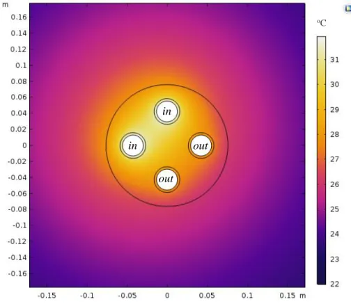
In fact, heat transfer from the fluid to the ground or vice versa, is a process where the concept of BHE thermal resistance between the fluid and the BHE surface appears. As illustrated by figure 2.9, heat transfer in a BHE depends on several factors such as the configuration of the pipes,
25
thermal properties of the circulating fluid, of grouting materials and of the surrounding ground, and the mass flow rate. The local heat transfer process within the BHE includes three components: convection between the inner wall of the U-tube pipes and the circulating fluid, conduction through the wall of U-tube pipes, and conduction through the grouting material. The thermal resistance corresponding to the first two thermal processes is considered as the thermal resistance of the U-tube pipe. The thermal resistive network for a single U-U-tube BHE is demonstrated in figure 2.10.
Figure 2.9. A BHE cross section.
The thermal resistance of the BHE can be expressed as follows:
b p gt
R R R (2.18)
where R is the thermal resistance of the grout and gt R refers to the thermal resistance of the U-p tube pipe and is computed as:
p cond conv
R R R (2.19)
where Rcond and Rconvstand for the conduction and convection heat transfer inside the pipe, respectively.
26
Figure 2.10. Thermal resistive network for a single U-tube BHE.
If one denotes by Tf the fluid bulk temperature, by Ts the external BHE wall surface
temperature and by ql the heat flux per unit length of the BHE (thermal power exchanged between the BHE and the ground), the thermal resistance of the BHE is defined as:
f s b l T T R q (2.20)
Since Tf and Ts are not uniform, and the real mean value of Tf is often not known, different
definition of the BHE thermal resistance, i.e., different ways of application of equation (2.20), have been proposed. These definitions differ on the method to calculate Tf and on selecting either
a 2D or a 3D domain to apply equation (2.20).
Lamarche et al. [56] have investigated the available methods to evaluate the BHE thermal resistance by a review paper. Recently, Zanchini and Jahanbin [57] have analyzed, by means of finite element simulations, the differences between the various definition of thermal resistance, for double U-tube BHEs. In addition, they have investigated the effects of the temperature distribution on the thermal resistance of double U-tube BHEs. The heat transfer process and the thermal resistance of a double U-tube BHE are analyzed in detail in chapters 3 and 7 of the present thesis.
2.5 Hybrid GCHP systems
Most building-plant systems have unbalanced seasonal heating and cooling loads. This circumstance can yield a decrease of the system performance of a GCHP system after some years. For instance, when a GCHP system is employed in a cooling-dominated building in a warm climate, more heat will be rejected to the ground than that extracted, on annual basis. This will
R in-out Tg R g-s, out R out-s R g-s, in Ts R in-s Ts Tf, out Tf, in
27
cause an increase of the ground temperature, which may deteriorate the performance of the GCHP system in a long term. Furthermore, a cooling-dominated building needs a BHE with larger size with respect to a situation with balanced loads. In a similar way, in a heating-dominated building, in a cold climate, a larger BHE field is needed to satisfy the higher heating demand; moreover, the ground will tend to cool down during the years, with a decrease of the system performance.
Figure 2.11. Schematic diagram of a HGCHP system with solar collector, presented in reference [44].
Hybrid Ground-Coupled Heat Pump (HGCHP) systems are an alternative way to increase the system performance and decrease the initial cost of the GCHP system, simultaneously. The HGCHP systems employ a supplemental heat rejecter/absorber which can reduce a significant amount of the heat rejected/extracted into/from the ground, in order to balance the ground thermal loads, leading to a better energy performance of the GCHP systems.
In recent years, remarkable studies have been done on the development of the various HGCHP systems. According to the Yang et al. [44], the main types of the HGCHP systems are:
HGCHP systems with supplemental heat rejecters HGCHP systems with hot water supply
HGCHP systems with solar collectors
Figure 2.11 shows a schematic diagram of a HGCHP system with solar collector [44].
A comprehensive study on different types of the HGCHP systems, design methods, and simulations for the HGCHP systems can be found in details in references [44, 58-61].
29
![Figure 2.1. U.S. annual primary energy consumption by source from 1950 to 2015, data according to EIA [1]](https://thumb-eu.123doks.com/thumbv2/123dokorg/8113675.125254/32.918.135.789.167.623/figure-annual-primary-energy-consumption-source-data-according.webp)
![Figure 2.4. Schematic of a GSHP system in heating/cooling mode, reported by EPA [12].](https://thumb-eu.123doks.com/thumbv2/123dokorg/8113675.125254/35.918.107.811.197.593/figure-schematic-gshp-heating-cooling-mode-reported-epa.webp)
![Figure 2.5. The installed capacity and annual utilization of geothermal heat pumps from 1995 to 2015 [15]](https://thumb-eu.123doks.com/thumbv2/123dokorg/8113675.125254/36.918.152.770.301.638/figure-installed-capacity-annual-utilization-geothermal-heat-pumps.webp)
![Figure 2.11. S chematic diagram of a HGCHP system with solar collector, presented in reference [44]](https://thumb-eu.123doks.com/thumbv2/123dokorg/8113675.125254/49.918.207.684.274.552/figure-chematic-diagram-hgchp-solar-collector-presented-reference.webp)
![Table 3.1. Shape factors for three different patterns of the shank spacing [66].](https://thumb-eu.123doks.com/thumbv2/123dokorg/8113675.125254/57.918.218.696.365.528/table-shape-factors-different-patterns-shank-spacing.webp)
![Table 4.1. The thermophysical properties adopted in Code I, taken from reference [91]](https://thumb-eu.123doks.com/thumbv2/123dokorg/8113675.125254/78.918.127.794.284.420/table-thermophysical-properties-adopted-code-i-taken-reference.webp)