Chance-Constrained Automated Test Assembly
Giada Spaccapanico Proietti, Mariagiulia Matteucci, Stefania Mignani University of Bologna
Bernard P. Veldkamp University of Twente
Abstract
Classical automated test assembly (ATA) methods assume fixed and known parameters, an hypothesis that is not true for estimates of item response theory parameters which are key elements in test assembly. To account for uncertainty in ATA, we propose a
chance-constrained version of the MAXIMIN ATA model which allows to maximize the α-quantile of the sampling distribution function of the test information function obtained by bootstrapping the item parameters. An heuristic based on the simulated annealing is proposed to solve the ATA model. The validity of the proposed approach is verified by simulated data and the applicability is verified by an application to real data.
Keywords: automated test assembly; uncertainty; chance-constrained; simulated annealing
Chance-Constrained Automated Test Assembly
In the field of educational measurement, tests should be designed and developed providing evidence of fairness, reliability and validity (American Educational Research Association et al., 2014). In order to make different measurements comparable, a test assembly process may be used to select items from an item pool and build test forms conforming to content and psychometric specifications. Thus, test assembly plays a crucial role in this field as it allows to control the entire protocol of the test production, from the item construction, since the features of the pool depend on the requirements on the final tests, to the final test building. Large testing programs, having better access to modern digital resources like sophisticated item banking systems, opened the possibility to improve their test assembly process by means of automated test assembly (ATA).
ATA differs from manual test assembly because the item selection is performed by optimizing mathematical models through specific solvers. Therefore, ATA has several advantages over manual test assembly. First of all, a rigorous definition of test
specifications will reduce the need to repeat some phases of the test development. More importantly, ATA is the only way to find optimal or near-optimal combinations of items starting from large item banks, for which manual assembly is not feasible due to the large number of possible solutions. As a consequence, ATA is fundamental to make
measurements comparable while reducing operational costs. A limit of classical
optimization models such as 0-1 linear programming (LP) models (see van der Linden, 2005), usually applied in ATA, is that they consider each model parameter as fixed or known. However, this assumption is not valid for parameter estimates, key elements in ATA models. In fact, most test assembly models are based on item response theory (IRT), which is used for estimating both the item parameters and the examinees’ ability.
Consequently, the estimated IRT item parameters and the item information function (IIF) are uncertain inputs in ATA models (Veldkamp et al., 2013). Mislevy et al. (1994), Patton et al. (2014), Tsutakawa and Johnson (1990), Xie (2019), Zhang et al. (2011), Zheng (2016)
discussed the consequences of uncertainty in item parameters on several aspects, such as ability estimation. In the ATA literature, relatively few studies focused on the issue of dealing with uncertainty by proposing robust alternatives to the classical optimization models (De Jong et al., 2009; Veldkamp & Paap, 2017; Veldkamp & Verschoor, 2019; Veldkamp, 2013; Veldkamp et al., 2013).
Our proposal in this paper is to incorporate uncertainty in the optimization model for simultaneous multiple test assembly which is the most seen in practice and in the literature (Ali & van Rijn, 2016; Debeer et al., 2017; van der Linden, 2005). We suggest a test
assembly model based on the chance-constrained (CC) approach (see Charnes & Cooper, 1959; Charnes et al., 1958) which allows to maximize the α-quantile of the sampling distribution of the test information function (TIF). The proposed model is an extension of the classical MAXIMIN ATA model (van der Linden, 2005, p. 69-70) in which the
minimum TIF among all the tests is maximized. The sampling distribution of the TIF is obtained by adopting the bootstrap technique in the calibration process (Bradley &
Tibshirani, 1993). In this way we ensure that, independently on the situation in which the calibration has been made, we have an high probability to have a certain, possibly low error in the ability estimation. For solving the ATA models, chance-constrained or not, we developed an algorithm based on the simulated annealing (SA), a stochastic meta-heuristic proposed by Goffe (1996). This technique can handle large-scale models and non-linear functions. All the proposed algorithms have been coded in the open-source framework Julia (Bezanson et al., 2017). In our novel model, the entire structure of uncertainty of the item parameters is taken into account and this is optimal with respect to the accuracy of the ability estimates.
The paper is organized as follows. Firstly, the key elements of IRT and ATA are reviewed discussing the issue of including uncertainty. Secondly, an introduction to the CC approach for solving optimization problems with uncertainty is provided. Then, the proposal of an ATA model, specifically a CC version of the MAXIMIN test assembly model, is developed
by discussing the retrieval of the TIF empirical distribution function by bootstrap and the heuristic based on SA for solving the model. Afterwards, the results of a simulation study are presented in order to compare our proposal to the existent approaches solved by the CPLEX 12.8.0 Optimizer (IBM, 2017). An application of our approach on real data taken from the 2015 Trends in International Mathematics and Science Study (TIMSS) data is shown. Concluding remarks end the paper.
Item Response Theory and Test Assembly Models
In educational and psychological measurement, IRT provides a good framework for ATA methods because, from the item parameter estimates describing the item psychometric characteristics, it is possible to derive the item Fisher information, a key object used to build optimal test in terms of accuracy of ability estimation.
Once the item parameters have been estimated for a given IRT model, it is possible to understand how precise the test is at various ranges of the latent ability by using the TIF, which is defined as the sum of the item Fisher information for all the items in the test. In fact, the TIF has a very favourable property that is the additivity (and hence linearity) over the items of a test. Given a test with k items, the TIF is equal to
I(θ) =
k X
i=1
Ii(θ), (1)
where Ii(θ) is the IIF for item i, with i = 1, ..., k, and θ ∈ (−∞, ∞) is the latent ability.
Expressions for the IIFs can be easily derived within the framework of IRT. For example, let assume binary response data, where the probability of item i endorsement Pi(θ) follows
the two-parameter logistic (2PL) model. In this case, the IIF of item i is equal to
Ii(θ) = a2iPi(θ)(1 − Pi(θ)) = a2i
exp(aiθ+bi)
[1 + exp(aiθ+bi)]2, (2)
where the item parameters ai and bi represent the discrimination and the easiness for item
The Fisher information function is a crucial element in test assembly because of its linearity and its easy interpretation. In general an ATA model is an optimization model composed by some constraints to be fulfilled and an objective function to maximize or minimize, where the test specifications are defined as the set of the desiderata considered for the test. Well defined test specifications can always be represented in the standard form of Table 1 as reported in van der Linden (2005, p. 40).
Table 1
Standard Form of a Test Assembly Problem
optimize Objective function subject to Constraint 1 Constraint 2 .. . Constraint N
Only one objective can be optimized at a time; if we have more than one function to optimize some tricks can be applied to transform the objectives into constraints. On the other hand, there is no upper limit for the number of constraints, provided that the solver can handle the problem. If at least one combination of items that meets all the constraints does exist, then the set of these combinations is the feasible set; otherwise, the model will be infeasible. The subset of tests in the feasible set that optimizes the objective function represents the optimal feasible solution.
Tests can be assembled merely through the selection of appropriate items out of an item bank; one way to do so is to use mathematical programming techniques like 0-1 linear programming (LP) or mixed integer programming (MIP) models by using commercial
solvers such as CPLEX (IBM, 2017) or Gurobi (Gurobi, 2018). Using these approaches the tests can be built by, for instance, maximizing the TIF at predefined θ points (MAXIMIN), or matching it with known optimal values (MINIMAX) with linear restrictions on the values of items properties (see van der Linden, 2005). In multiple simultaneous test assembly, if we need to assemble T tests and each test has to meet a target for its
information function at K ability points the problem has at least T × K objectives. In this setting, given an item pool of I items, the MAXIMIN ATA model is specified by adding to the standard form of Table 1 the following set of objective and constraints:
maximize y (objective) (3a)
subject to I X i=1 Ii(θkt)xit≥ yRkt, ∀t, k ∈ Vt, (3b) y ≥ 0,
where Ii(θkt) is the IIF for item i at the ability level θk in test t, xit is a decision variable
which takes value 1 if the item i is assigned to test t and 0 otherwise, Rkt is the relative
target for each θk in test t, with t = 1, ..., T and k = 1, ..., K, i.e. the set of ability points
for test t in which we want to control the shape of the TIF. The Rkt may be chosen equal
among the tests, i.e. Rkt = Rk0t0 with t 6= t0 and ∀k = k0 ensuring the parallelism.
Uncertainty in Test Assembly
In the context of test assembly, the optimization models commonly used for item selection do not consider the inaccuracy of the estimates of item parameters (van der Linden, 2005). For example, the MAXIMIN ATA model is based on the TIF which appears in the
objective function, being the goal of the optimization model. The TIF is the sum of the IIFs, which in turn depend on the item parameter estimates and are considered as known quantities. This approach of ignoring uncertainty derived from the estimation process may lead to several issues such as infeasibility, e.g. the impossibility to find T parallel tests that
have TIFs inside a fixed interval around the targets. Another issue is the misinterpretation of the assembly results. For example, if the calibration algorithm had produced biased estimates for the item parameters, the IIFs are not accurate enough and, consequently, the TIF of the assembled test might be underestimated or overestimated. As a consequence, the accuracy of ability estimates may be compromised. Regarding the latter issue, a good test assembly model would consider the variation of the item parameter estimates in order to build test forms in a conservative fashion, i.e., it would produce tests with a maximum plausible lower bound of the TIF.
Several attempts to include uncertainty in the test assembly models have been done by developing robust proposals. Starting from the conservative approach of Soyster (1973), where the maximum level of uncertainty is considered for 0–1 LP optimization, De Jong et al. (2009) proposed a modified version where one posterior standard deviation is
subtracted from the estimated Fisher information to take the calibration error into account in ATA. This approach was adopted also in Veldkamp et al. (2013), where the
consequences of ignoring uncertainty in item parameters are studied for ATA models. In addition, Veldkamp (2013) investigated the approach of Bertsimas and Sim (2003), who developed a robust method for 0-1 LP models by including uncertainty only in some of the parameters, in the assembly of linear test forms. More recently, Veldkamp and Paap (2017) proposed to include the uncertainty related to the violation of the assumption of local independence in ATA for testlets. Finally, Veldkamp and Verschoor (2019) discussed robust alternatives for both ATA and computerized adaptive testing (CAT).
The mentioned ATA robust approaches consider the standard error of the estimates and a protection level Γ that indicates how many items in the model are assumed to be changed in order to affect the solution. In a sense, the uncertainty is treated in a deterministic way and, given Γ, the solution is adjusted by adopting a conservative approach, as standard errors are the maximum expression of uncertainty of the estimates. Chance-constraints (or probabilistic constraints) appears to be a natural solution to the mentioned problem. In
fact, they are among the first extensions proposed in the stochastic programming
framework to deal with constraints where some of the coefficients are uncertain (Charnes & Cooper, 1963; Krokhmal et al., 2002).
Chance-Constrained Modeling
The CC approach (Charnes & Cooper, 1959; Charnes et al., 1958) is a method to deal with sources of uncertainties in optimization problems by adjusting a conservative parameter α, the risk level, to modulate the level of fulfilment of some probabilized constraints enabling to relax or to tighten the feasibility of the problem.
The CC modeling has been deeply explored in the financial scientific field. In fact, in risk management and reliability applications the decision maker must select a combination of assets for building a portfolio by maximizing their utility function. Since the prices of instruments are usually random variables, the theory of choice and portfolio optimization under risk was born (see Rockafellar & Uryasev, 2000, 2001). In the past five decades, this sort of problems followed the expected mean-variance approach (Chen, 1973; Freund, 1956; Scott Jr & Baker, 1972). In particular, the utility function is defined in terms of the
expected mean and variance of the returns or of the prices of the instruments which are uncertain coefficients in the linear objective or constraints of the optimization model. More recently, instead, the regulations for finance businesses require to reformulate the problem in terms of percentiles of loss distributions. These requirements gave rise to the theory of chance-constraints, also called probabilistic constraints, originally proposed by Charnes and Cooper (1959).
The probabilistic constraints include coefficients which are assumed to be randomly
distributed and are subject to a some predetermined threshold α controlling the fulfilment of constraints. By modifying α, it is possible to relax or tighten some constraints
mixed-integer optimization problem can be represented by arg max x f (x) (4) subject to gj(x) ≤ 0 j = 1, . . . , J x ∈ Zp× Rn−p,
where f (·) is the objective function to be optimized, gj(·) is the function expressing the
constraints, J is the number of constraints, and x is the vector of p integer and n − p continuous optimization variables. Both f (·) and g(·) are scalar functions.
The optimization domain is D = dom(f ) ∩TJj=1dom(gj) and the set
X = {x : x ∈ D, gj(x) ≤ 0 ∀j} is the feasible set, i.e. a solution x is feasible if it is in the optimization domain and it satisfies the constraints. Starting from (4), a
chance-constrained reformulation adds the following set of H constraints:
P [gh(x, ξ) ≤ 0] ≥ 1 − α h = 1, . . . , H, (5)
where ξ is a vector of random variables. This formulation seeks a decision vector x that minimizes the function f (x) while satisfying the chance constraints gh(x, ξ) ≤ 0 with
probability at least equal to (1 − α). Such constraints imply having a function to compute (or better approximate) the probability and a solver to deal with that function.
CC models represent a robust approach to optimization. However, despite they were proposed in the 1950s, CC models are still hard to be solved. An issue is the general non-convexity of the probabilistic constraints. In fact, even if the original deterministic constraints gh(x, ξ) with non-random ξ are convex, the respective chance-constraints may
be non-convex. In general they are usually untractable because, even if they are convex, the quantiles of the random variables are difficult or impossible to compute (see
Nemirovski & Shapiro, 2006). Examples of approximations of chance-constraints are the sample average approximation (Ahmed & Shapiro, 2008), based on linearization, and the case of random variables following a known multivariate distribution with known
parameters. For the first case, a big-M approach is needed to deal with the indicator function bringing numerical instability in the optimization. The second approach instead imposes strong distributional assumptions (see Kataria et al., 2010). Since they are based on the Chebyshev’s inequality, they require a modest number of elements in the
summations to achieve the convergence, and they need also a solver to deal with
second-order conic constraints, the most difficult type of convex functions to be optimized. All the mentioned formulations increase exponentially the number of optimization
variables, thus they are not suitable for large-scale models.
Other approaches rely on the discretization of the random variables. The model is optimized in all possible scenarios (i.e. realizations of the random variables) and, as a consequence, these approaches do not fit to problems with a large number of random variables because all the patterns must be considered (Margellos et al., 2014; Tarim et al., 2006; Wang et al., 2011). In finance, such models are called value at risk (VaR) and they are usually characterized by non-concavity and hence computational intractability, except for specific cases where returns are known to have an elliptical distribution, see for example Vehviläinen and Keppo (2003) or McNeil et al. (2005).
Chance-Constrained Automated Test Assembly
In order to develop a conservative approach including uncertainty on item parameters into the ATA model, we propose a stochastic optimization for the MAXIMIN test assembly model based on the CC method. Under this approach, the TIF is not considered as a fixed quantity but as a random variable. As it is explained further on, the distribution of the TIF is retrieved by using the bootstrap technique.
Whenever a MAXIMIN principle is applied, the chance constraints can be seen as
percentile optimization problems (Krokhmal et al., 2002). In fact, the probability in (5) is replaced by the α-th percentile of the distribution function of gh(x, ξ) and these percentiles
By considering the MAXIMIN model (3a), the constraints (3b) involved in the
maximization of the TIF are replaced by the chance-constrained equivalents as follows P " I X i=1 Ii(θkt)xit ≥ y # ≥ 1 − α, ∀t, k, (6)
where t = 1, . . . , T are the test to be assembled and θkt are the ability points in which the
TIF of the test form t must be maximized, with k = 1, ..., K. In order to simplify the notation, the relative targets Rkt have been omitted (or equivalently put equal to one) but
the extension is straightforward. We call the model (6) chance-constrained MAXIMIN, or CCMAXIMIN. The key element of this model is, again, the information function which is assumed to be random.
The CCMAXIMIN model allows to maximize the expected precision of the assembled tests in estimating the latent trait of the test-takers at pre-determined ability points with a high confidence level if the α is chosen to be close to zero. In terms of probability we can say that the constraints in (3b) must be fulfilled with a probability at least equal to (1 − α). By adjusting the confidence level, it is possible to relax or tighten the attainment of the chance-constraints to reflect a specific conservative attitude, i.e. a small α means an high level of conservatism while, on the contrary, a large α means an almost complete relaxation of the constraints. This is the main novelty of the CCMAXIMIN model with respect to the robust approach proposed by Veldkamp (2013), Veldkamp et al. (2013) who, instead, perform a worst-case optimization. Once the chance-constraints have been defined, a way to evaluate the probability in (6) must be found in order to quantify the feasibility of the solution. To solve this problem, some methods rely on assumptions regarding the
probability distribution of ξ, such as the multivariate normal (Kim et al., 1990). Ahmed and Shapiro (2008) try to approximate the probability distribution using samples of the random variable of interest by a Monte Carlo simulation, which is a specific case of a scenario generation where all the scenarios have the same probability of occurrence. We decided to use the Monte Carlo method because of its flexibility and adaptability to our problem.
The proposed CCMAXIMIN model for ATA is based on the empirical distribution of the TIFs of the assembled tests. Therefore, our random variable is the TIF of a test form, a statistic depending on the IRT item parameter estimates, such as the discrimination and the easiness, which are uncertain. There are different ways to sample from the distribution function of this random variable: given the standard errors of the estimates, the samples can be uniformly drawn from their confidence intervals as in the robust model of
(Veldkamp, 2013); otherwise, if a Bayesian estimation is carried on, the samples in the Markov chain can be used.
In this paper, a bootstrap procedure is performed resampling the response data and
generating a sample of estimates for each item parameter. At the end of this phase, the IIF for all the items in the pool, at predefined ability points, is computed using the
bootstrapped samples. These quantities are then used in the CCMAXIMIN model to compute the α-quantiles of the TIFs and the model is optimized by looking for the best combination of items which produces the tests with the highest quantiles. A percentile optimization model would maximize a reasonable lower bound of the TIF, its α-quantile, approximated by the dαRe-th ranked value of the TIF computed on the R bootstrap replications of the estimates of item parameters. In the following sections, the details of the retrieval of the empirical distribution function of the TIF by the bootstrap and the
heuristic proposed to solve the model are explained.
Empirical Measure of the TIF
The test forms built using the CCMAXIMIN model should have the maximum possible empirical α-quantile of their TIFs. The optimality in this sense will ensure that the assembled tests are conservative in terms of accuracy of ability estimation (indeed, the TIF) taking into account the uncertainty in the estimates of the item parameters. A standard approach to extract the uncertainty related to the item parameter estimates could be to sample a high number of plausible values of the item parameters in the
confidence intervals built using the standard errors and, subsequently, compute the related IIFs at target θ points. This may be an optimal starting point to assemble robust tests (see Veldkamp, 2013; Veldkamp et al., 2013), but it has its own downsides as a uniform interval of plausible values is assumed. Another attempt to account for the influence of sampling error in the Bayesian framework has been made by Yang et al. (2012) who proposed a multiple-imputation approach with the aim to better measure the latent ability of a respondent.
Our approach is based on bootstrapping the calibration process; in particular, the observed vectors of responses coming from the full sample (one vector for each test-taker) are
resampled with replacement R times and the item parameters are estimated for each sample. In this way, it is possible to preserve the natural relationship of dependence between the items and, given the ability targets, it is possible to compute their IIFs. After that, given a set of items, we can build a test form and compute its TIF for each of the R replications. The resulting sample constitutes the empirical distribution function of the TIF.
More formally, let ξ1, . . . , ξR be an independent identically distributed (iid) sample of R realizations of a I-dimensional random vector ξ, its respective empirical measure is
ˆ FR:= R−1 R X r=1 ∆ξr, (7)
where R is the number of bootstrap replications, with r = 1, ..., R, and ∆ξr denotes the mass at point ξr, with ∆ξr(A) = 1 when ξr ∈ A. Hence ˆFR is a discrete measure assigning
probability 1/R to each sample. In this way we can approximate the probability in the left-hand side of (6) by replacing the true cumulative distribution function of ξ by ˆFR.
Let 1(−∞,0]{x} : R → R be the indicator function of x in the interval (−∞, 0], i.e.,
1(−∞,0]{x} = 0, if x > 0 1, if x ≤ 0. (8)
sample ξ1, . . . , ξR of our random vector, we can rewrite P [gh(x, ξ) ≤ 0] =EF h 1(−∞,0]{gh(x, ξ)} i ≈EFˆR h 1(−∞,0]{gh(x, ξ)} i (9) =1 R R X r=1 1(−∞,0]{gh(x, ξr)}.
That is, the chance-constraint is evaluated by the proportion of realizations for which gh(x, ξ) ≤ 0 in the sample.
Adopting the same principle to the left-hand side of the chance-constraints in (6), the CCMAXIMIN model can be approximated by
arg max x y subject to 1 R R X r=1 1[y,∞){Ir(θkt)0xt} ≥ 1 − α, ∀t, k, (10) gj(xt) ≤ 0 ∀j, t, xt∈ {0, 1}I, y ∈ R+, ∀t.
Model (10) is characterized by the following issues: it is clearly non-convex because of the chance-constraints (see Rockafellar & Uryasev, 2000, 2001, for the demonstrations) and the indicator function is not well handled by commercial solvers. To overcome these problems we propose to solve the model by an heuristic which is described next.
The Heuristic
Since the proposed CCMAXIMIN model for ATA cannot be approximated by a linear formulation, an heuristic based on the SA (Goffe, 1996) has been developed. This technique can handle large-scale models and non-linear functions. The mechanism to incorporate the constraints in the objective function is inspired by the work of Stocking and Swanson (1993) who used the hinge function and more in general, the Lagrange relaxation.
Through the Lagrange relaxation (Fisher, 1981), the violation (i.e. the absolute deviation from the constraints of the analyzed solution) is included in the objective function. In this
way, it is possible to solve a simplified version of the problem and to obtain an upper bound for the optimal solution of the initial problem. In fact, even if the problem is highly infeasible, the solver returns the most feasible combination of variables that maximizes the modified objective function. Given the general mixed-integer optimization model (4), its Lagrange relaxation will be:
arg max x f (x) − λ X j gj(x) ∀j (objective) (11) x ∈ Zp× Rn−p,
where λ is the Lagrange multiplier, which has the role to weight the violations of the constraints in the new objective function. We opt for a modification of the previous model to allow the violations to interfere in the optimization only when the constraints are not met. The (11) will become:
arg max x f (x) − λX j max [0, gj(x)] ∀j (objective) (12) x ∈ Zp× Rn−p,
In the case of test assembly, the relaxation of the classical linear ATA model is still linear. We summarize this approach by an example of the Lagrange relaxation applied to a single test assembly model with an objective function to maximize. Suppose we have two set of indices mu ∈ Mu and ml ∈ Ml for upper and lower bound constraints and m ∈ Mu∪ Ml.
We can rewrite the relaxed version of a standard single test assembly model as follows: maximize β I X i=1 qixi− (1 − β) X m∈Mu∪Ml zm (objective) (13a) subject to I X i=1 cimuxi− ubmu ≤ zmu, ∀mu (constraints) (13b) − I X i=1 cimlxi+ lbml ≤ zml, ∀ml (constraints) (13c)
xi ∈ {0, 1}, ∀i, (decision variables)
zm ∈ R+, ∀m, (violations)
where (1 − β), with 0 ≤ β ≤ 1, is a modified version of the Lagrange multiplier which is explained in detail below. Note that any linear constraint with upper or lower bounds can be represented as a generic constraint either of the form (13b) or (13c). For example, the minimum length of the test can be written as (13c) and the maximum length as (13b) where the ci are all equal to 1, lb = nmin and ub = nmax. The definition of zm as a positive
real number let the solver look for solutions that makes the sum of zm goes to zero and
hence it tries to satisfy all the constraints.
The weight β can be chosen by the test assembler to control the trade-off between
optimality and feasibility of the final solution. For example, if a solution producing more accurate ability estimates is preferred at the expense of the fulfillment of tougher
constraints, the β should be chosen close to 1. Viceversa, if all the constraints should be fulfilled, a lower β should be selected. An optimal choice of β can be done by analyzing the results of several optimization attempts. The choice of β will depend on the level of
feasibility of the model and to the highest value that the TIF can assume, given the item pool.
On the other hand, adopting the SA algorithm, more than one area of the solution space is explored avoiding to being trapped in a local optimum. Unfortunately, the SA has the disadvantage that is hardly able to find the feasible space of a problem, this is why we
decided to start our heuristic by a filling up sequential phase in which the worst performing test, both in terms of optimality and feasibility, is filled-up with the best item available in the item pool. After the item has been assigned, the process is repeated until all the tests have reached their maximum length, i.e. they are all filled-up. Once the first step is performed, we process the solution with the SA principle. If a feasible set of tests is still not available, the solver will first take into account only the feasibility of the model and then it proceeds introducing the TIF optimality. At each step of the optimization, the tests are altered by removing or switching one of the already selected items with the ones still available in the pool. We maintain the latter solution if the computed objective function satisfies the normalized Boltzmann factor proper of the SA algorithm (Goffe, 1996), otherwise we proceed to the next step where another item or test is altered. The cooling scheme is implemented by selecting a starting temperature and decreasing it by a
geometric factor at each step. When no improvement is achieved after 100 alterations, we save the last best solution and we reheat the environment by setting the temperature to its starting value and we move forward another area of the space of x that we call
neighbourhood. The algorithm stops whenever one of the termination criteria, e.g. time limit or relative objective function tolerance, is met. All the proposed algorithms have been coded in the open-source framework Julia (Bezanson et al., 2017).
The result of the heuristic is a set of solutions with length equal to the number of neighbourhoods explored. It is also possible to decide how many of these areas must be evaluated just in terms of feasibility, and how many in terms of optimality. In this way, the test assembler has a wider choice of optimally assembled tests in terms of other features not considered in the assembly model, such as content validity.
Simulation Study
The performance and benefits of the CCMAXIMIN test assembly model (10) are
using probabilistic methods in the field of ATA models in terms of conservatism of the test solution. In particular, this purpose is assessed by comparing the quantile of the TIFs obtained by our CCMAXIMIN model, solved in Julia, and by the classical MAXIMIN one (3a) solved in CPLEX through the JuMP interface1. We refer to a model without the
Lagrange relaxation as the strict model, instead, when the Lagrange relaxation is applied the model is called relaxed. Our heuristic only handles the relaxed version of the model, with CPLEX, instead, we can define the model also in its strict version.
The data needed for assembling the CC tests consist of the sample of the IIFs computed at the predetermined ability points, θkt, of each item in the pool, namely the Ir(θkt), for
r = 1 . . . , R. These quantities are obtained by bootstrapping the item parameters. A 2PL model is assumed.
The CCMAXIMIN model (10) is solved and the best value of its objective function among all the explored neighbourhoods is retained together with the amount of infeasibility given by the sum of all the violations (which is zero by definition in the strict model). In order to show that our heuristic effectively reaches a near optimal solution in an uncertain
environment we compare the minimum, among all the T tests, of the empirical α-quantile of the TIF computed at θ = 0, i.e. mint[Q(T IFt(0), α)]. As already mentioned, considering
that CPLEX is not able to solve the CCMAXIMIN model, the quantiles are computed on the items chosen by solving the classical MAXIMIN ATA model (3a).
Test Specifications
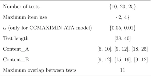
The just mentioned models are solved under different settings, such as the number of test forms and the confidence level α. The assembly is performed in a parallel framework, i.e. all the tests must meet the same constraints. Two fictitious categorical variables, content_A and content_B, with three possible categories each, are simulated to constrain the tests to have a certain content validity. The complete set of test settings is summarized in Table 2. 1 http://www.juliaopt.org/JuMP.jl/0.18/
Table 2 Test Settings
Number of tests {10, 20, 25}
Maximum item use {2, 4}
α (only for CCMAXIMIN ATA model) {0.05, 0.01}
Test length [38, 40]
Content_A [6, 10], [9, 12], [18, 25]
Content_B [9, 12], [15, 19], [9, 12]
Maximum overlap between tests 11
The constraint described in Content_A, for example, requires that each test must have from 6 to 10 items having the first category of the variable content_A, from 9 to 12 items having the second category, etc... Different combinations of the first three settings in Table 2 (number of tests, maximum item use and α) create four cases to be investigated for the classical MAXIMIN ATA model and eight cases for the CCMAXIMIN ATA model in an increasing order of complexity and/or size of the model. The hyperparameters for the SA algorithm have been chosen as follows: we start with a temperature equal to 1.0 since we do not want the solver to go too far from the last explored neighbourhood and, at every step we decrease the temperature with a 0.1 geometric cooling parameter; at the beginning of the optimization we perform one fill-up phase only taking into account the feasibility of the model; then we proceed looking for the most optimal combination of items by
randomly selecting one item in all the tests to be removed or switched. The imposed termination criterion is limited to the amount of time needed for solving the model which is equal to 1000 seconds. This criterion is also valid for the CPLEX solver. We noticed that the fill-up phase produces solutions with a deviation of around 3.0 or 4.0 and the peak of TIF is around 10.0 so we chose a β equal to 0.1 to balance the two summands of the objective function.
The optimization has been performed on a desktop PC with an AMD Ryzen 5 3600X 6-Core Processor and 32 GB of RAM. We ran the Julia package in parallel with respect to the neighbourhoods to be explored, starting Julia with 4 cores. The steps addressed in the simulation study are described herewith:
1. Simulate a pool of I=250 items. Item parameters (2-parameter logistic): a ∼ LN (0, 0.25) (discrimination), b ∼ N (0, 1) (easiness). Contents: content_A={type1,type2,type3}, content_B={type4,type5,type6}.
2. Generate the responses of N = 3000 students with θ ∼ N (0, 1). Calibrate the items with a marginal maximum likelihood estimation approach with an unbalanced design (500 test-takers per item).
3. Re-calibrate the items R = 500 times on N∗ = N respondents resampled with replacement (bootstrap). Compute the IIFi(r)(0) for r = 1, . . . , R and i = 1, . . . , I. 4. Set the constraints as in 2 and optimization features as explained in the previous
paragraph.
5. For the 4 cases taken into account:
(a) Solve the classic MAXIMIN model (3a) in its strict and relaxed versions by CPLEX.
(b) For α ∈ {0.01, 0.05}: Solve the CCMAXIMIN model (10) by our heuristic.
Results
In Table 3 and Table 4, the minimum among the T tests, of the α-quantiles, Q(T IFt(0), α),
and of the true values of the TIFs, T IFt∗(0), obtained with the different approaches are reported. The highest values, so the best, are formatted in bold.
Table 3
mint[Q(T IFt(0), 0.05)](mint[T IFt∗(0)])
Model Strict MAXIMIN Relaxed MAXIMIN CCMAXIMIN
Case T Item use max CPLEX CPLEX Our solver
1 10 4 13.588(13.028 ) 13.592(12.795 ) 13.699(13.074 ) 2 10 2 10.179(10.183 ) 10.180(10.203 ) 10.230(10.353 ) 3 20 4 10.105(9.610 ) 10.154(10.018 ) 10.192(10.084 ) 4 25 4 8.705(8.817 ) 8.622(8.529 ) 8.829(8.725 ) Table 4 mint[Q(T IFt(0), 0.01)](mint[T IFt∗(0)])
Model Strict MAXIMIN Relaxed MAXIMIN CCMAXIMIN
Case T Item use max CPLEX CPLEX Our solver
1 10 4 13.218(13.028 ) 13.134(12.795 ) 13.298(13.043 )
2 10 2 9.813(10.183 ) 9.780(10.203 ) 9.948(9.957 )
3 20 4 9.679(9.610 ) 9.746(10.018 ) 9.987(9.889 )
4 25 4 8.375(8.817 ) 8.375(8.529 ) 8.554(8.849 )
The results are overall very promising. First of all, it was not necessary to report the total violation of the solutions since the constraints are always profitably fulfilled. This proves that our heuristic is able to find the feasible space of the problem and it is not sensible to alterations of the test specifications. Moreover, it is consistent with the definition of the empirical quantiles since it never produces a set of tests with a minimum 0.01-quantile higher than the minimum 0.05-quantile. Secondly, we observe the closeness of the true TIF, i.e. the objective function computed on the true values of the item parameters, to the value of the objective function obtained optimizing the CCMAXIMIN model. Thus,
maximizing the true value of the TIF, it’s able to approximate it very well, giving to the test assembler a better idea of how much the tests are accurate in estimating future abilities given the current uncertainty in item parameters.
At the end, the distance from the true TIFs observed in the tests assembled by the
analyzed ATA models is summarized in Table 5 for all the cases. In particular, we averaged across the tests the differences between the true TIFs and the TIFs estimated on the full sample for the strict and relaxed classic MAXIMIN model, and the differences between the true TIF and the α-quantiles of the TIF for the CCMAXIMIN model. We consider the TIFs at θ = 0 because it is the ability point in which it is maximized.
Table 5
Average Difference from the True TIF at θ = 0.
Case/Model Strict MAXIMIN Relaxed MAXIMIN CCMAXIMIN CCMAXIMIN
1 1.000 1.082 0.091 -0.186
2 0.341 0.341 -0.320 -0.575
3 0.350 0.345 -0.321 -0.527
4 0.165 0.173 -0.412 -0.669
The positive discrepancies for the classical MAXIMIN model highlight the main worrisome aspect we are trying to present in this paper: the TIF is likely to be overestimated and, if we do not take into account the uncertainty in the item parameters in the test assembly process, we are possibly overestimating the expected error of ability estimation of the assembled tests. On the other hand, with the CC approach, a nonhazardous position can be adopted by maximizing a lower bound of the true TIF, its α-quantile, which is derived from the item calibration error. The latter statement is supported by negative or barely positive differences between the true TIF and their observed quantiles. Furthermore, the difference increases when α is reduced showing that the level of conservativeness of the solution is, as expected, negatively correlated with α and hence customizable.
Application to Real Data
The data used in this application come from the 2015 TIMSS survey, a large-scale standardized student assessment conducted by the International Association for the Evaluation of Educational Achievement (IEA). Since 1995, this project monitors trends in mathematics and science achievement of 39 countries every four years, at the fourth and eighth grades and at the final year of secondary school. TIMSS 2015 was the sixth of such assessments. Further information regarding this study are available at the TIMSS 2015 web page. We selected the Italian sample of grade 8 students for the science test
(n = 4479). The choice of the subject was driven by the availability of items, in fact the science item bank was larger than the mathematics one. The original item pool has been filtered removing derived and polytomous items and retaining only original binary items. The final dataset contains 234 items divided into the following categorical features: 4 content domains (69 Biology items, 57 Chemistry items, 58 Physics items, and 50 Earth Science items), 3 cognitive domains (98 Applying items, 88 Knowing items, and 48 Reasoning items), and 4 topics (110 items with topic 1, 80 items with topic 2, 33 items with topic 3, 11 items with topic 4). Furthermore, some items are grouped in 27 units. The design is unbalanced so missing values appear in the data. The item parameters were estimated according to the 2PL model. After the calibration, we performed a
non-parametric bootstrap with R = 500 replications on the item parameters and we computed the IIF at θ = 0 for all the items in the pool.
In the calibrated item pool, the discrimination parameter estimates range from 1e-05 to 4.708, with a mean of 0.920 and a median of 0.867. There are two items with the minimum allowed value of the discrimination estimate. On the other hand, the easiness parameter estimates range from -4.340 to 4.546, with mean and median equal to 0.071 and 0.025, respectively.
The final matrix of the IIFs contains 234 × 500 samples. Subsequently, we solved the CCMAXIMIN model by using the proposed approach and imposing the following
specifications, in terms of test constraints, which were inspired by the features of the tests administered in the TIMSS 2015. In detail, a set of T = 14 tests with length from 29 to 31 items is assembled. The already mentioned friend sets are included in the assembly as constraints. We imposed the tests to have at least 6 items for each content domain (Biology, Chemistry, Physics and Earth Science), a minimum of 8 items in the Applying and Knowing cognitive domains, and a minimum of 7 items in the Reasoning cognitive domain. The first and the second topic must be present at least 10 times in each test form. The forms must contain at least 2 items on the third topic and 1 item on the fourth topic. Each item can be used in at most 3 test forms. The overlap must be less or equal to 15 items between adjacent forms, 5 items between forms at distance equal to 2 (e.g. form 1 and 3 can have an overlap of maximum 5) and, no overlap is allowed for all the pairs at distance greater than 2. For the CCMAXIMIN model we chose α = 0.05 and a β = 0.01. The last choice is motivated by the high level of infeasibility of the model. We excluded from the assembly 11 items which had IRT b parameter higher than 3 or lower than -3. This helped the solver to assemble the tests with a TIF peaked where the θ is around 0. After we included all the specifications in the model, we run the optimization algorithm which implements our heuristic. We selected the same termination criteria as in the simulation study. Before the time limit had been reached, the algorithm explored 4
neighbourhoods: the first and the second neighbourhoods were not feasible, their objective function reached the value of 15.84 and 14.85 respectively. These values are positive, which means that most of the inequalities imposed with the constraints were false. This fact can be easily confirmed by looking at the infeasibility vector returned by our solver which showed for the first two neighbourhoods values higher than 0. On the other hand, the third and the fourth neighbourhood had a negative value of the objective function equal to -0.0455 and -0.0484, respectively.
Thus, the best solution is produced within the last neighbourhood where the smallest 0.05-quantile among the tests is equal to 4.843. The assembled tests fulfil all the constraints
as it can be seen from Table 6. Also constraints on overlap and item use are satisfied. Table 6
TIMSS Data, Features of the Test Forms Assembled by the CCMAXIMIN ATA Model.
Test (t) 1 2 3 4 5 6 7 8 9 10 11 12 13 14 Length 29 29 29 30 29 29 29 29 29 30 30 29 29 29 Content Domain Biology 9 6 7 6 10 10 10 10 7 7 9 8 9 10 Chemistry 6 6 8 9 6 7 6 6 6 8 9 8 7 6 Physics 8 9 8 6 7 6 7 7 8 8 6 7 7 7 Earth Science 6 8 6 9 6 6 6 6 8 7 6 6 6 6 Cognitive Domain Applying 12 13 10 12 12 13 12 8 11 13 12 10 12 10 Knowing 9 8 12 11 9 9 10 12 11 9 11 11 9 11 Reasoning 8 8 7 7 8 7 7 9 7 8 7 8 8 8 Topic 1 11 10 11 11 11 10 12 15 16 15 17 13 10 15 2 10 12 10 10 10 10 10 10 10 10 10 10 13 10 3 7 6 6 7 6 8 6 3 2 4 2 2 2 3 4 1 1 2 2 2 1 1 1 1 1 1 4 4 1
The maximized α-quantiles together with the TIF at θ = 0 computed on the sample are reported in Table 7. A graphical representation of the sampling distributions of the TIFs in shown in Figure 1.
Table 7
Test Information Function of the Assembled Tests for TIMSS Data at θ = 0 Test (t) Q(T IFt(0), 0.05) T IFt(0) 1 4.853 5.157 2 4.843 5.166 3 4.893 5.243 4 4.861 5.175 5 4.999 5.325 6 4.876 5.178 7 4.893 5.276 8 4.854 5.259 9 4.865 5.243 10 4.857 5.175 11 4.862 5.286 12 4.880 5.355 13 4.877 5.308 14 4.852 5.185
The resulting TIFs and quantiles do not considerably differ among the test forms, this is a signal that the model reached an optimal solution which is very proximal to the global one. However, the TIF is rather low, and this is due to the high infeasibility of the model and because the values of the IIFs at θ = 0 were also low. We suppose that the items considered in this application are not suitable to evaluate the average ability of the Italian sample but they are most appropriate to measure the ability of more proficient students. This can be seen also from the TIFs of the assembled tests which have their peaks for θ > 0 (Figure 1). Analyzing the sampling distribution of the TIFs of the assembled tests illustrated in Figure 1, we can notice that the TIF computed on the full sample is always higher than the
Figure 1
Examples of TIFs of the Assembled Tests 1 and 2. TIF Estimated on the Full Sample (solid black) against Quantiles.
−4 −2 0 2 4 0 2 4 6 8 θ T I F (θ ) Max 75-Qle Median 25-Qle α− Qle Min estimated Test 1 −4 −2 0 2 4 0 2 4 6 8 θ T I F (θ ) Max 75-Qle Median 25-Qle α− Qle Min estimated Test 2
0.05-quantile. Thus, for example, we could say that there is a low possibility that test 2 produces estimates of the ability of an examinee with a true θ = 0 with a standard error of measurement greater thanq(1/4.843) = 0.454.
Concluding Remarks
In this work, a chance-constrained version of the MAXIMIN ATA model, namely
CCMAXIMIN ATA, has been defined. Our novel test assembly model is able to deal with the uncertainty in item parameters affected by calibration errors, which, in practice, can be relevant especially for small sample sizes. In particular, we tried to take into account the entire structure of the uncertainty of a test optimal with respect to its accuracy in
estimating the individual ability. This task is performed by approximating the distribution function of the TIF using the bootstrapped replicates of the item parameter estimates. The last step reformulates the classic MAXIMIN ATA model in a percentile optimization
problem which is a sub-category of the CC models. To deal with the non-linear formulation of the proposed CCMAXIMIN model, we developed an heuristic based on the SA principle for finding the optimal conservative tests. In this way, unlike classical optimization
techniques, it is also possible to handle large-scale models.
The results of a simulation study show that the CCMAXIMIN ATA model, together with our heuristic, maximizes an adjustable conservative version of the test information
function, i.e. its α-quantile, where α can be arbitrarily chosen from the test assembler. The latter has been empirically proven to be a lower-bound to its true counterpart when α is taken as a small value such as 0.05 or 0.01. Thus, the use of the sampling distribution function of the TIF along with the CC formulation gives a better representation of the accuracy of the tests in estimating future abilities and reduces the potential side effects of the calibration errors. In contrast, with the classic method which uses the full sample estimates, the TIF is often higher than the true one giving dangerous misinterpretations. At the end, an application on real data coming from the TIMSS survey demonstrated that
References
Ahmed, S., & Shapiro, A. (2008). Solving chance-constrained stochastic programs via sampling and integer programming. In Z.-L. Chen & S. Raghavan (Eds.), 2008 tutorials in operations research: State-of-the-art decision-making tools in the information-intensive age (pp. 261–269). Informs.
Ali, U. S., & van Rijn, P. W. (2016). An evaluation of different statistical targets for assembling parallel forms in item response theory. Applied Psychological Measurement, 40 (3), 163–179.
American Educational Research Association, American Psychological Association, & National Council on Measurement Education. (2014). Standards for educational and psychological testing. American Educational Research Association.
Bertsimas, D., & Sim, M. (2003). Robust discrete optimization and network flows. Mathematical Programming, 98 (1-3), 49–71.
Bezanson, J., Edelman, A., Karpinski, S., & Shah, V. B. (2017). Julia: A fresh approach to numerical computing. SIAM Review, 59 (1), 65–98.
Bradley, E., & Tibshirani, R. J. (1993). An introduction to the bootstrap. Chapman & Hall/CRC.
Charnes, A., & Cooper, W. W. (1959). Chance-constrained programming. Management Science, 6 (1), 73–79.
Charnes, A., & Cooper, W. W. (1963). Deterministic equivalents for optimizing and satisficing under chance constraints. Operations Research, 11 (1), 18–39. Charnes, A., Cooper, W. W., & Symonds, G. H. (1958). Cost horizons and certainty
equivalents: An approach to stochastic programming of heating oil. Management Science, 4 (3), 235–263.
Chen, J. T. (1973). Quadratic programming for least-cost feed formulations under probabilistic protein constraints. American Journal of Agricultural Economics, 55 (2), 175–183.
De Jong, M. G., Steenkamp, J.-B. G. M., & Veldkamp, B. P. (2009). A model for the construction of country-specific yet internationally comparable short-form marketing scales. Marketing Science, 28, 674–689.
Debeer, D., Ali, U. S., & van Rijn, P. W. (2017). Evaluating statistical targets for
assembling parallel mixed-format test forms. Journal of Educational Measurement, 54 (2), 218–242.
Fisher, M. L. (1981). The lagrangian relaxation method for solving integer programming problems. Management Science, 27 (1), 1–18.
Freund, R. J. (1956). The introduction of risk into a programming model. Econometrica, 24 (3), 253–263.
Goffe, W. L. (1996). SIMANN: A global optimization algorithm using simulated annealing. Studies in Nonlinear Dynamics & Econometrics, 1 (3), 169–176.
Gurobi. (2018). The gurobi optimizer [version 8.0].
IBM. (2017). Ibm ilog cplex optimization studio [version 12.8.0].
Kataria, M., Elofsson, K., & Hasler, B. (2010). Distributional assumptions in chance-constrained programming models of stochastic water pollution. Environmental Modeling and Assessment, 15, 273–281.
Kim, C. S., Schaible, G. D., & Segarra, E. (1990). The deterministic equivalents of chance-constrained programming. Journal of Agricultural Economics Research, 42 (2), 30–39.
Krokhmal, P., Palmquist, J., & Uryasev, S. (2002). Portfolio optimization with conditional value-at-risk objective and constraints. Journal of Risk, 4, 43–68.
Margellos, K., Goulart, P., & Lygeros, J. (2014). On the road between robust optimization and the scenario approach for chance constrained optimization problems. IEEE Transactions on Automatic Control, 59 (8), 2258–2263.
McNeil, A. J., Frey, R., & Embrechts, P. (2005). Quantitative risk management: Concepts, techniques and tools (Vol. 3). Princeton University Press.
Mislevy, R. J., Wingersky, M. S., & Sheehan, K. M. (1994). Dealing with uncertainty about item parameters: Expected response functions. ETS Research Report Series,
1994 (1), i–20.
Nemirovski, A., & Shapiro, A. (2006). Convex approximations of chance constrained programs. SIAM Journal on Optimization, 17, 969–996.
Patton, J. M., Cheng, Y., Yuan, K.-H., & Diao, Q. (2014). Bootstrap standard errors for maximum likelihood ability estimates when item parameters are unknown.
Educational and Psychological Measurement, 74 (4), 697–712.
Rockafellar, R. T., & Uryasev, S. (2000). Optimization of conditional value-at-risk. Journal of Risk, 2, 21–42.
Rockafellar, R. T., & Uryasev, S. (2001). Conditional value-at-risk for general loss distributions. ISE Dept., University of Florida.
Scott Jr, J. T., & Baker, C. B. (1972). A practical way to select an optimum farm plan under risk. American Journal of Agricultural Economics, 54 (4), 657–660.
Soyster, A. L. (1973). Convex programming with set-inclusive constraints and applications to inexact linear programming. Operations Research, 21, 1154–1157.
Stocking, M. L., & Swanson, L. (1993). A method for severely constrained item selection in adaptive testing. Applied Psychological Measurement, 17 (3), 277–292.
Tarim, S. A., Manandhar, S., & Walsh, T. (2006). Stochastic constraint programming: A scenario-based approach. Constraints, 11 (1), 53–80.
Tsutakawa, R. K., & Johnson, J. C. (1990). The effect of uncertainty of item parameter estimation on ability estimates. Psychometrika, 55 (2), 371–390.
van der Linden, W. J. (2005). Linear models for optimal test design. Springer.
Vehviläinen, I., & Keppo, J. (2003). Managing electricity market price risk. European Journal of Operational Research, 145 (1), 136–147.
Veldkamp, B. P., & Paap, M. C. S. (2017). Robust automated test assembly for testlet-based tests: An illustration with analytical reasoning items. Frontiers in Education, 2 (63), 1–8.
Veldkamp, B. P., & Verschoor, A. J. (2019). Robust computerized adaptive testing. In B. Veldkamp & C. Sluijter (Eds.), Theoretical and practical advances in
computer-based educational measurement (pp. 291–305). Springer.
Veldkamp, B. P. (2013). Application of robust optimization to automated test assembly. Annals of Operations Research, 206 (1), 595–610.
Veldkamp, B. P., Matteucci, M., & de Jong, M. G. (2013). Uncertainties in the item parameter estimates and robust automated test assembly. Applied Psychological Measurement, 37 (2), 123–139.
Wang, Q., Guan, Y., & Wang, J. (2011). A chance-constrained two-stage stochastic program for unit commitment with uncertain wind power output. IEEE Transactions on Power Systems, 27 (1), 206–215.
Xie, Q. (2019). The impact of collateral information on ability estimation in an adaptive test battery (Doctoral dissertation) [https://doi.org/10.17077/etd.njvy-42a6]. University of Iowa.
Yang, J. S., Hansen, M., & Cai, L. (2012). Characterizing sources of uncertainty in item response theory scale scores. Educational and Psychological Measurement, 72 (2), 264–290.
Zhang, J., Xie, M., Song, X., & Lu, T. (2011). Investigating the impact of uncertainty about item parameters on ability estimation. Psychometrika, 76 (1), 97–118. Zheng, Y. (2016). Online calibration of polytomous items under the generalized partial