Automated Configuration of Offline/Online Algorithms: an Empirical Model Learning Approach

(1)

ALMA MATER STUDIORUM · UNIVERSITY OF BOLOGNA

SCHOOL OF ENGINEERING AND ARCHITECTURE

DEPARTMENT of COMPUTER SCIENCE and ENGINEERING (DISI)

TWO-YEAR MASTER’S DEGREE in COMPUTER ENGINEERING

MASTER’S THESIS In

Intelligent Systems M

Automated Configuration of Offline/Online

Algorithms: an Empirical Model Learning

Approach

Supervisor: Candidate:

Prof. MILANO MICHELA MINERVA MICHELA

Co-supervisors:

Dr. DE FILIPPO ALLEGRA Dr. BORGHESI ANDREA

Academic Year 2019/2020 Session III

(2)

(3)

iii

Abstract

The energy management system is the intelligent core of a virtual power plant and it manages power flows among units in the grid. This implies dealing with optimization under uncertainty because entities such as loads and renewable energy resources have stochastic behaviors. A hybrid offline/online optimization technique can be applied in such problems to ensure efficient online computation.

This work devises an approach that integrates machine learning and optimization models to perform automatic algorithm configuration. It is inserted as the top component in a two-level hierarchical optimization system for the VPP, with the goal of configuring the low-level offline/online optimizer.

Data from the low-level algorithm is used for training machine learning models - decision trees and neural networks – that capture the highly complex behavior of both the controlled VPP and the offline/online optimizer. Then, Empirical Model Learning is adopted to build the optimization problem, integrating usual mathematical programming and ML models.

The proposed approach successfully combines optimization and machine learning in a data-driven and flexible tool that performs automatic configuration and forecasting of the low-level algorithm for unseen input instances.

(4)

iv

List of Figures

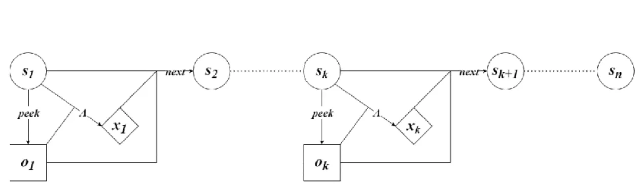
Figure 1: Virtual power plant schema. ... 8 Figure 2: Online stochastic optimization is modeled as an n-stage problem. All the functions involved in the model are represented: peek, next, and A. At stage 𝑘: 𝑠_𝑘 is the system state, 𝑥𝑘 the decision taken, and 𝑜𝑘 are the observed variables - the related observed uncertainty is 𝜉_𝑘 -. ... 14

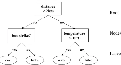
Figure 3: Decision tree with depth two. The target of the prediction is the means of transport to reach a destination – a categorical target. Features are the distance to the destination, the weather temperature on that day and the presence of a bus strike. ... 34 Figure 4: Decision Stump. Same classification problem of Figure 3: the target of the prediction is the means of transport to reach a destination. ... 34

Figure 5: Inference in a Decision Tree. In red the sequence of decisions for a sample that is labeled as “walk”. ... 36

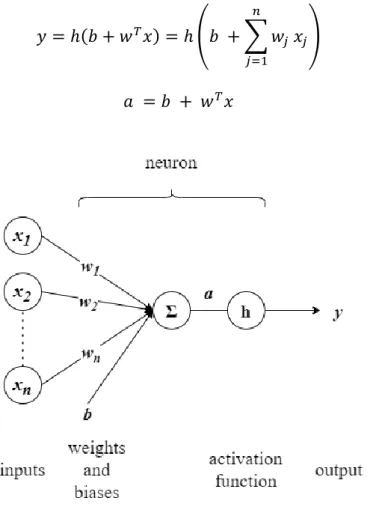
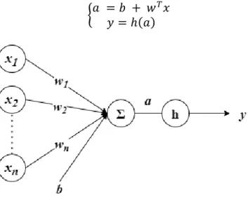
Figure 6: Neuron schema. The input is an n-dimensional vector x and the output is the prediction y. 𝑎 is the neuron activity. The bias 𝑏 can be treated as an additional weight 𝑤_𝑛+1 with input signal constant to 1 to simplify the notation. We adopt this notation hereinafter. ... 40

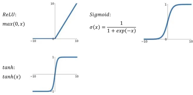
Figure 7: Commonly used activation functions: Sigmoid, ReLU, and tanh. ... 41 Figure 8: General high-level architecture of a multi-layer feed-forward neural network. ... 42

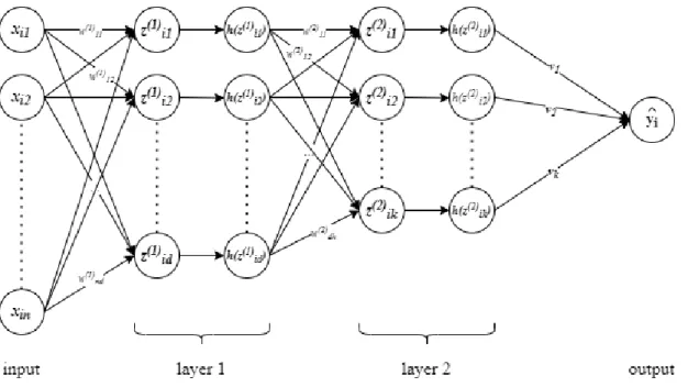
Figure 9: Two-layers neural network; all signals are detailed for the input sample 𝑖. Every circle represents a signal: input features 𝑥_𝑖, hidden features 𝑧_𝑖(1) = 𝑊(1)𝑥_𝑖 and 𝑧_𝑖(2) = 𝑊(2)ℎ(𝑊(1)𝑥𝑖), output 𝑦̂𝑖. Although the output 𝑦̂𝑖 is a scalar here, it might as well be a vector and, in that case, 𝑣 is a matrix.. ... 42

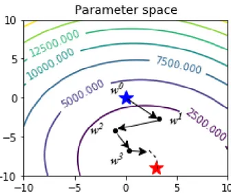
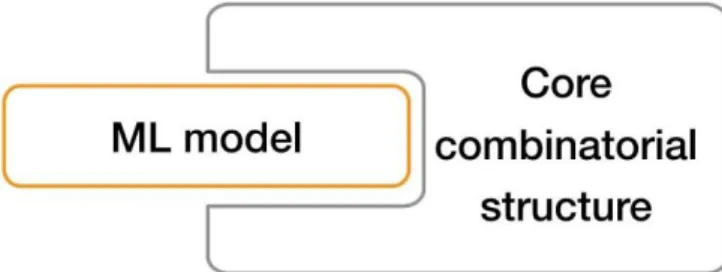
Figure 10: Gradient Descent in a two-dimension parameter space. The blue star is the starting point (i.e. the value of parameters at the beginning 𝑤0), while the red star is the optimum. Arrows represent the descent performed in each GD iteration... ... 45 Figure 11: In EML, the optimization problem is composed of the (original) core combinatorial structure and a empirical machine learning model. ... 53

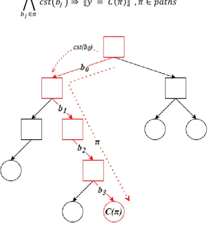
Figure 12: Representation of a DT in EML. A path 𝜋 in the DT is represented by a logical implication involving all conditions 𝑐𝑠𝑡(𝑏_𝑗) along the path, leading to the label 𝐶𝜋. ... 56

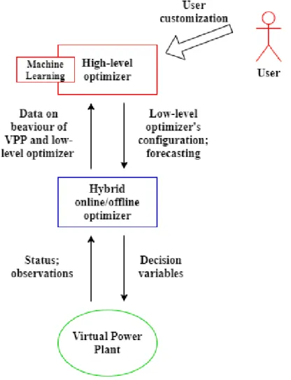
Figure 13: Neuron schema in EML, adopting a similar notation to section 3. .. 58 Figure 14: General overview of the entire VPP optimization system. The low-level hybrid offline/online optimizer performs stochastic optimization for the VPP. The high-level optimizer allows both decision-making on the configuration and

(8)

viii

performance forecasting for the low-level optimizer; it is data-driven, flexible, and customizable by the user. ... 62

Figure 15: Composition of the custom combinatorial optimization model. It builds over a set of basic variables and constraints. Empirical ML models are integrated via EML. The objective and additional constraints are interactively specified by the user to fit the specific use case. ... 90

(9)

ix

List of Graphs

Graph 1: Pair plot for number of traces, solution cost, and time. ... 65 Graph 2: Average solution cost across all 100 instances, for each value of the number of traces. The variance is also reported in each bar. ... 67

Graph 3: Standard deviation for the solution cost across all 100 instances, for each value of the number of traces. ... 67

Graph 4: Average online resolution time across all 100 instances, for each value of the number of traces. The variance is also reported in each bar. ... 67

Graph 5: Standard deviation for the online resolution time across all 100 instances, for each value of the number of traces. ... 68

Graph 6: Scatterplot between average memory and number of traces. The instance id is colored. ... 69

Graph 7: Scatterplot between maximum memory and number of traces. The instance id is colored. ... 69

Graph 8: Feature importance for the RF. Features 0-4 are PV, 5-9 are Load, and 10 is cost. ... 73

Graph 9: Feature importance for the RF. Features 0-4 are PV, 5-9 are Load, 10 is cost, and 11 is time. ... 75

Graph 10: Feature importance for the RF. Features 0-4 are PV, 5-9 are Load, 10 is time, 11 is cost, and 12 is memory. ... 79

Graph 11: Feature importance for the RF model that aggegates scores of single regressors. In order: score of the regressors for average memory, cost, and time. .... 80

Graph 12: Number of traces and Cost suggested by the optimizers under different memory bounds. The proposed ML models are compared. For each memory costraint value, the result is averaged across all instances and time constraint values. ... 100

Graph 13: Number of traces and Cost suggested by the optimizers under different time bounds. The proposed ML models are compared. For each time costraint value, the result is averaged across all instances and memory constraint values. ... 100

Graph 14: nTraces and Cost suggested by the DT11-based optimizer under different memory bounds, averaged across all instances, for each time constraint value. ... 103 Graph 15: nTraces and Cost suggested by the DT11-based optimizer under different time bounds, averaged across all instances, for each memory constraint value. ... 103 Graph 16: Optimization results (Memory, Time, nTraces, and Cost) for each proposed optimizer on instance #13. Different constraint values are imposed for the cost improvement w.r.t. baseline. ... 106

(10)

x

Graph 17: Optimization results (Memory, Time, nTraces, and Cost) for the DT11-based optimizer on several instances. Different constraint values are imposed for the cost improvement w.r.t. baseline. ... 107

Graph 18: Pair plot for solution cost and time, where the number of traces is colored. ... 116

Graph 19: Pair plot for number of traces and resolution time, where the solution cost is colored. ... 116

Graph 20: Pair plot for number of traces and solution cost, where the resolution time is colored. ... 116

Graph 21: Scatterplot between solution cost and nTraces for one instance (#1). ... 117 Graph 22: Scatterplot of the average cost per nTraces. For each value of nTraces we average all solution costs. ... 117

Graph 23: Scatterplot of the average number of traces per cost. For each value of cost we average all number of traces. ... 117

Graph 24: Scatterplot of the average number of traces per cost, with binned cost. We perform binning on the cost with a range of 5, i.e. we split the cost’s domain in intervals of length 5 and we group together all data points whose cost is within an interval. For each interval we average the number of traces. ... 117

Graph 25: Scatterplot of solution cost and number of traces, with the instance id colored. ... 118

Graph 26: For the first 20 instances, scatterplot of solution cost and number of traces, with the instance id colored. This helps to shed light on how the instance influences the relationship between cost and nTraces. ... 118

Graph 27: Feature importance for the RF regressor that takes as features PV (0-4), Load (5-9), and average memory (10). A RF Classifier is used beforehand for dimensionality reduction of both PV and Load. ... 121

(11)

xi

List of Tables

Table 1: Test set performance for the best regressors that predict nTraces using

cost and (if applicable) PV/load as features. ... 73

Table 2: Test set performance for regressors that predict nTraces using time as feature. ... 75

Table 3: Test set performance for regressors that predict nTraces using time, cost and (if applicable) PV/load as features. ... 76

Table 4: Test set performance for the best regressors that predict nTraces using average memory and (if applicable) PV/load as features. ... 77

Table 5: Test set performance for regressors that predict nTraces using maximum memory as feature. ... 77

Table 6: Test set performance for the best regressors that predict nTraces using all the remaining variables as features. ... 79

Table 7: Test set performance for the best regressors that predict nTraces using all the remaining variables as features. ... 81

Table 8: Test set performance of experimental DTs on the standardized dataset. ... 83

Table 9: Test set performance, depth, and training time of DT5. ... 85

Table 13: Test set performance and training time of NNs. ... 86

Table 14: Information on times and dimensions of combinatorial optimization models with embedded ML models. ... 92

Table 15: Comparative experiments for DT9, DT11, DT15, and NN. For each problem we report objective and constraints, resolution time for the high-level optimizer and, for each variable of interest, the solution value. ... 96

Table 16: Average resolution time for the high-level optimizer. ... 99

Table 17: Standard deviation of each solution value across all instances, averaged across all experiments (i.e. constraints’ values) for each ML model. ... 101

Table 18: Solutions of the high-level optimization model based on DT11, averaged across all instances. The first two columns (memc and timec) are the constraints. The remaining columns are the solution found: in this specific problem, nTraces are the variable suggested by the system whereas memory, time, and cost represent forecasts. ... 102

Table 19: Average resolution time for the high-level optimizer. ... 104

Table 20: Average maximum cost improvement found by each optimizer. .... 105

Table 21: Statistics on each column of the dataset containing records of runs of the hybrid offline/online algorithm. ... 115

(12)

xii

Table 22: Test set performance for classifiers that predict nTraces using cost, PV, and load as features. ... 119

Table 23: Test set performance for regressors that predict nTraces using cost and (if applicable) PV/load as features. ... 120

Table 24: Test set performance for regressors that predict nTraces using average memory and (if applicable) PV/load as features. ... 121

Table 25: Test set performance for regressors that predict nTraces using all remaining variables as features. The model is unified, namely, a unique regressor takes all features and predicts nTraces. ... 122

Table 26: Test set performance on all dataset’s normalizations for experimental DTs that do not use PV/Load as features. ... 123

Table 27: Test set performance on all dataset’s normalizations for experimental DTs that use PV/Load as features. ... 123

Table 28: Hyperparameters selected for the NN models. Some of them (in blue) are embedded into the combinatorial optimization problem and used in optimization experiments. ... 124

Table 29: Complete comparative experiments for DT9, DT11, DT15, NN. For each problem we report objective and constraints, resolution time for the high-level optimizer and, for each variable of interest, the solution value. ... 126

(13)

xiii

List of Acronyms

• Adam: Adaptive moment estimation. • ANN: Artificial neural network. • DER: Distributed energy resource. • DT: Decision tree.

• DS: Decision stump.

• EML: Empirical Model Learning. • EMS: Energy management system. • GD: Gradient descent.

• GRS: Greedy recursive splitting. • KDE: Kernel density estimate. • KNN: K-nearest neighbors.

• LASSO: Least absolute shrinkage and selection operator. • LR: Linear regression.

• MAE: Mean absolute error.

• MILP: mixed-integer linear programming- • ML: Machine learning.

• MSE: Mean squared error. • NN: Neural network. • nTraces: Number of traces.

• PCA: Principal component analysis. • PV: RES generation power.

• ReLU: Rectified linear unit. • RES: Renewable energy source. • RBF: Radial basis function • RF: Random forest.

• SGD: Stochastic gradient descent. • SVM: Support vector machine. • VPP: Virtual power plant.

(14)

1

Introduction

Smart grids are the evolution of electrical grids, interconnected infrastructures that deliver electrical energy to consumers. They integrate novel power sources into a distributed energy resources scenario. Smart grids leverage state-of-the-art control and information techniques to perform monitoring, control, and forecasting on the complex network of distributed entities, named virtual power plant. The core of the VPP is the energy management system; it is the orchestrator of such a large system and it manages its power flows. By virtue of the EMS, a smart grid enables enhanced energy efficiency, flexibility, security, and reliability in the power distribution; it promotes green power sources thus helping the environment and it allows money savings by adopting smart energy management.

The EMS in a VPP decides power flows in the grid and it operates under a specific objective, usually the minimization of operational costs. This is a problem of optimization under uncertainty because a smart grid integrates elements with stochastic behavior, e.g. renewable energy resources and loads. Hybrid offline/online algorithms can be applied to perform online optimization, namely, to decide power flows in real-time given the real conditions of the system. They adopt hefty stochastic optimization algorithms but shift part of their computation offline to reduce online costs. An offline/online technique is based on the expensive offline computation of a contingency table; it contains information on possible online scenarios called traces. In the online step, a very efficient fixing heuristic makes decisions guided by the contingency table; it adjusts offline-computed solutions to actual conditions. The number of traces guiding the fixing heuristic is a fundamental parameter to configure; it balances a tradeoff between solution quality and computation cost.

This work devises an approach to perform automatic configuration of the offline/online algorithm for new unseen instances. It introduces a combinatorial optimization problem on top of the offline/online method, resulting in a two-levels

(15)

2

hierarchical optimization system for the VPP. We want to define problem-specific objectives and constraints for the low-level optimization, for example concerning solution quality, online computation time, or resources. These are entailed in the high-level optimization problem. The proposed approach is used ahead of the online step to guide its design or get forecasts about its performance on unseen instances. It is an automatic tool for the configuration of the low-level algorithm that allows one to automatically decide or predict its parameters, run-time, or computational resources based on desired constraints and objectives.

The high-level optimizer captures the behavior of the controlled system, both the VPP and the hybrid offline/online algorithm. We leverage machine learning techniques, with a focus on decision trees and neural networks, to model the highly complex relationships between variables involved in the system.

The proposed approach leverages Empirical Model Learning to integrate empirical ML models and combinatorial optimization problems. Machine learning models that capture real-world relationships among variables are embedded in the optimization problem via EML; once encoded, they are used by the solver to generate solutions and boost the resolution process. The EML-based approach allows a flexible and completely data-driven design of the optimization model; it does not require specific knowledge about the VPP system or the hybrid optimization process, and it removes the need of a manually-crafted modeling phase by domain experts. EML brings together declarative models from optimization research and predictive models from machine learning, and it shows that optimization in complex real-world systems is possible.

We perform a preliminary study on machine learning techniques to assess how the relationships among variables are captured by different models. Then, we build decision trees and neural networks and we finally embed them in combinatorial optimization models. We compare optimization models based on DTs and NNs on several examples to shed light on their strengths and weaknesses. Finally, we apply different high-level optimizers, modeled using trees with distinct hyperparameters, on two real-world use cases.

(16)

3

Chapter 1 Virtual Power Plant

1.1 Smart Grid

Production, provisioning and consumption of electricity has been an important matter of research since the 18th century. The provisioning infrastructures currently used across the world to distribute power descend from the first alternating current (AC) system studied by Nikola Tesla with Westinghouse Electric in the late 1880s. The generation of electricity was localized around communities in a time when the energy demand was ridiculous compared to today, namely, few lightbulbs and power-alimented devices. A limited number of significant changes were made to the power distribution networks ever since. The “centralized top-down” power grid is designed for a unidirectional delivery of electricity to consumers. Power is generated in few large power plants, and from these locations it is distributed to customers through the power grid infrastructure. These systems are not designed for the continuously rising demand of the 21st century; the centralized design implies energy losses, in particular for long distances, together with significant construction and maintenance costs. Moreover, regular electrical grids do not meet the need of flexibility and they do not exploit the significant amount of data and resources available nowadays.

In recent years both production and consumption of energy have been advancing rapidly. Electrical grids have evolved with a progressive shift towards decentralized generation of energy. The development of several new energy resources allows production of sufficient amounts of energy to support the always-growing demand of energy. The introduction of green resources also meets the necessity of switching to environment friendly energy sources to reduce human’s footprint on a growingly impacted Earth. Moreover, consumers’ products and needs are changing in this direction: new smart sensors, devices, and smart appliances are available to consumers at large scale. An increasing number of products are becoming part of the electric

(17)

4

networks; an important example of this phenomenon is the growing market of electric vehicles.

This evolution is happening in parallel with large changes in computational capabilities available to humans. Technologies like cloud computing and big data techniques allow generation, storing, and elaboration of massive amounts of data. In the meantime, Artificial Intelligence (AI) allows scientists to use these data for analyzing and forecasting tasks in several different applications.

Finding themselves in between these two worlds, smart grids represent the modern evolution of regular electrical grids and assumed a role of increasing importance in both industrial and academic research. According to the European Union Regulation 347/2013 [1], “‘Smart grid’ means an electricity network that can

integrate in a cost efficient manner the behavior and actions of all users connected to it, including generators, consumers and those that both generate and consume, in order to ensure an economically efficient and sustainable power system with low losses and high levels of quality, security of supply and safety”.

A smart grid integrates distributed energy resources (DERs), both conventional sources and new types such as renewable resources (RESs). DERs represent the most important factor for decentralized generation and consumption of energy. They can be generation systems - both renewable and non-renewable, such as wind and solar power plants, biomass plants, gas generators, and conventional energy generation sources -, energy storage systems (ESS) or loads - such as building loads -. DER elements that are peculiar in smart grids are energy microgeneration entities; for example, a building that produces, stores, and shares energy generated through renewable sources.

Smart grids enable the most recent technologies to be integrated in the power system, both for production and consumption. Some examples are green energy sources such as wind and solar energy units for production, or smart home devices and electric vehicles for consumption.

Smart grids overcome the mono-directionality of the old infrastructure. They introduce a two-way dialog where not only electricity but also information is

(18)

5

exchanged between producers and customers. Data resulting from this communication is used by the systems for management purposes.

Smart grids use digital information, automation, and control technologies to increase energetic efficiency (namely, use less energy), provide flexibility and ensure security and reliability of the electric grid. They integrate smart technologies for monitoring and forecasting on all actors involved in the grid, from producers to smart appliances and devices. They leverage technology and data to increase economic efficiency for customers and to increase sustainability of the power system.

1.2 Virtual Power Plant

In a smart grid, several decentralized entities are connected and interact in a complex way. This sophisticated system must be orchestrated in order to achieve maximum efficiency while maintaining reliability. The network control structure must evolve to be able to handle distributed power resources, to ensure the flexibility requested to energy systems, to meet the needs of increasingly complex customer devices and to manage the variability of RESs. virtual power plants (VPPs) come into play in this important role.

A VPP is a distributed power plant; it aggregates and manages units connected to the electrical grid to produce, store, and use energy, allowing them to operate as a unified power plant. It clusters and orchestrates several little distributed energy resources, generating a more flexible and secure energy supply compared to a conventional power system. A VPP is able to generate the same amount of power of a large standard central power plant; however, it achieves this by aggregating and managing an entire network of DERs. Units in a VPP can be scattered across hundreds of private, commercial, and industrial locations, concentrated in a single area. This rich aggregation of micro energy assets is combined into a single entity, operating in the same manner of a conventional power plant, by means of a centralized control system. The VPP leverages the bidirectional flow of information of its smart grid: it receives

(19)

6

power measurements, capacity, and availability information from DERs [2] and uses them to efficiently orchestrate utilities.

The VPP allows DERs to participate in the energy market and to provide grid ancillary services, such as power reserve or frequency regulation, allowing to enhance the power system’s stability. It enhances both flexibility and stability in the power grid by providing services to better match supply/demand and allowing traditional utilities to plan and optimize production efficiency. Compared to a conventional energy management system, a VPP encourages a more dynamic and diverse energy market and it facilitates the use of cleaner energy sources. It increases economic returns for entities in the grid; this encourages more renewable installations, leading to a further push towards a sustainable energy supply. The VPP con operate so as to optimize energy flows over time, leading to economic savings both for consumers and for producers. Additionally, the structure itself of a VPP decreases energy loss in transportation because generation and consumption are localized in a specific area.

1.3 Energy Management System

The core of the intelligent VPP is the energy management system (EMS). The EMS manages loads, storages, and generators. It coordinates power flows among all entities and can perform forecasting and optimization for the entire grid.

This system leverages state-of-the-art techniques in information technology to identify optimum power dispatch, for example real time large data transfer, advanced forecast with smart algorithms and optimization strategies. Data science and machine learning algorithms are used to generate accurate predictions for power generation, load demand and electricity pricing forecast.

The EMS can balance provision fluctuations by turning up or down the energy supply to suit both the energy demand and the production. As energy demands constantly changes over time during the day, utilities must turn power on and off depending on the amount of energy needed at a specific moment.

(20)

7

VPP addresses uncertainty leveraging on the EMS. Power plants based on RESs introduce a new modus operandi named “feed it and forget it” [3] that adds complexity to the VPP operation. RESs have a stochastic and uncontrollable behavior; they produce and inject power into the electric network not following the demand, but according to external variables such as the time in the day, period in the year and weather conditions. This behavior makes it difficult to integrate the power generated by RES-based plants. Conventional power plants or large storage systems are used to balance both the demand of loads and the variable generation introduced by RESs. The smart grid provides the data and automation that enable RESs to put energy into the grid and optimize its use; the EMS plays a key role by managing all the entities interacting in this network.

The energy management system is also responsible for optimization in a VPP. It can operate by minimizing generation costs or maximizing profits. The cost of energy depends on availability and it fluctuates during the day; electricity is more expensive to provide at peak times because secondary - often less efficient - power plants must be operative to meet larger demands. Optimization algorithms in a VPP leverage power forecasts and compute the optimum projected power dispatch for all its energy assets. This enables units to operate optimally for maximum return. Based on the current energy price and the status of DERs, the EMS decides how much energy should be produced, which generator should be used to produce the required energy and whether the surplus energy should be stored or sold to the energy market external to the VPP. Sophisticated smart grids enable utilities, in cooperation with customers, to manage and moderate electricity usage especially during peak demand times, resulting in reduced costs for utilities and costumers. Moreover, by encouraging to defer electricity usage away from peak hours, electricity production is more distributed throughout the day, reducing costs and inefficient fluctuations. The EMS also performs forecasting on the smart grid systems, to predict and manage energy usage under different conditions and over time, leading to lower production cost.

The EMS plays an important role in assuring not only optimization but also stability and reliability of the grid. It manages electricity consumption in real time and

(21)

8

receives continuous feedback information from DERs themselves. This greater insight allows the use of techniques to reduce, predict and overcome outages. Forecasting is used to predict energy fluctuations due to disruptions in the VPP caused by utility failures or weather conditions; the system can automatically identify problems in rerouting and restore power delivery.

Figure 1: Virtual power plant schema. From ABB1_.

(22)

9

Chapter 2 Optimization Under Uncertainty

The increasing amount and complexity of Distributed Energy Resources connected to the smart grid has brought some challenges to the management of the power system network. New optimization models are required to guide and control distributed units in the grid. In this context, virtual power plants play an important role by ensuring that the power produced, stored, and consumed by DERs is efficiently managed.

The energy management system of the VPP orchestrates entities and power flows with a certain objective, e.g. aiming at minimizing costs. In this process, the EMS considers several uncertainty factors that come into play in the smart grid, such as power generation from renewable resources. Uncertainty must be addressed so as not to compromise the reliability of the system. As a consequence, the optimization process performed by the EMS to decide power flows is a problem of making decisions under uncertainty, i.e. stochastic optimization.

This chapter provides information on methods for optimization under uncertainty and on how a VPP system can be modeled in optimization problems. These techniques represent the low-level optimizer inside the system proposed in this work.

2.1 Robust Optimization in VPPs

In [4] an optimization model to be employed in the EMS is presented. The proposed approach aims at minimizing operational costs by deciding the optimal planning of power flows for each point in time. It integrates into the model the necessary uncertainty elements.

(23)

10

The optimization approach is composed of two steps. The first is an offline day-ahead phase (a robust step) that computes optimized demand shifts to minimize the expected daily operating costs of the VPP. It uses a robust approach based on scenarios for modeling uncertainties present in the system, e.g. stemming from RESs such as wind or solar sources, and produces an estimated cost.

The second step is an online greedy optimization algorithm (greedy heuristic). It receives as inputs the optimized load shifts and it manages power flows in each timestamp in the VPP based on the real situation, with the aim of reaching the optimal real cost. This approach uses the optimized shifts produced by the first step to minimize, for each timestamp, the real operational cost, while allowing to fully cover the optimally shifted energy demand and avoiding the loss of energy actually produced by RES generators. It computes the real optimal value for the power flow variables based on the actual realization of uncertain quantities, assuming that the shifts have been planned by leveraging the first offline step; each timestamp is optimized one at time.

The first robust step produces good optimized shift that do not significantly deviate, in terms of cost, from the model with no uncertainty. On the other hand, according to the results in [4], the greedy step causes a significant loss in the quality of results.

2.2 Anticipatory Optimization Algorithms

A two-step optimization algorithm allows online decision-making in a VPP. The basic online step leverages a greedy heuristic that causes degradation in the quality of solutions, as mentioned in section 2.1. A way to improve the performance consists in replacing the greedy heuristic with a sampling-based stochastic anticipatory algorithm [5]. These algorithms were first developed for offline optimization, but they can be leveraged in online situations.

(24)

11

Offline applications are the usual focus for methodologies proposed in literature for stochastic optimization [6]. These methods usually base their optimization process on building a statistical model of future uncertainty, leveraging a sampling process that yields a set of scenarios. The Sample Average Approximation method [7] [8] solves stochastic optimization by adopting a simulation approach based on Monte Carlo simulation. It approximates the expected objective function of the stochastic problem with a function estimate on random samples; then, it solves with deterministic optimization techniques the resulting sample average approximation problems, in order to obtain candidate solutions for the original stochastic problem. This approach finds robust solutions by relying on one copy of the decision variables for each scenario and linking them via non-anticipativity constraints. It converges under reasonable assumptions and outperform greedy approaches.

Recent computational improvements in resources and techniques allowed the application of similar approaches to online optimization, leading to stochastic online

anticipatory algorithms. Optimization problems under uncertainty usually benefit

from an online approach; uncertainty progressively resolves in the online phase and decisions are made reacting and adapting to actual external events, allowing the discovery of robust high-quality solutions. An algorithm is called anticipatory if at some point it anticipates the future, namely, it makes use of information on the future to make decisions. While the algorithm at each time stamp can not fully know the future, i.e. the situation in following timestamps, it makes decisions based on inputs and possible future outcomes; future outcomes are estimated relying on possible scenarios delineated by past observations and current inputs.

Online anticipatory algorithms are effective [9] [10] but often computationally expensive, making them problematic as online decisions must be taken in short time frames. They usually rely on sampling to generate scenarios that estimate possible developments for a fixed number of future steps, called look-ahead horizon. Larger sample size leads to higher accuracy but also bigger problems to solve. This represents a problem because many use cases prescribe to make online decisions under strict time

(25)

12

constraints. As a consequence, methods must be adopted to improve the efficiency of these methodologies; for instance, a conditional sampler can be exploited to generate scenarios taking into account past observations [11].

In many situations a significant amount of information is available before the online execution, in an offline phase where time constraints are relaxed. For example, an EMS might have access to energy production and consumption forecast for the smart grid. This offline information can be exploited for characterizing uncertain elements, for sampling likely outcomes, called scenarios, and for supporting online optimization strategies.

2.3 Hybrid Offline/Online Anticipatory Algorithms

Optimization under uncertainty can combine an online and an offline phase in order to achieve good solution quality with minimum online cost. A simple approach to tackle such problems is to deal with the offline and online phase separately, respectively via a sampling-based method and a heuristic. However, [12] [13] show that substantial improvements can be obtained by treating these two phases in an integrated fashion.

In particular, [13] proposes three methods that leverage an offline preparation phase to reduce the online computational cost of a sampling-based anticipatory algorithm, while maintaining the quality in the solution. The methods build on an online sampling-based anticipatory algorithm but shift part of the computation to an offline stage. The proposed hybrid offline/online approaches combine:

1. A technique to identify the probability of future outcomes based on past observations.

2. An expensive offline computation of a contingency table; it contains pre-computed solutions to guide online choices.

(26)

13

3. An efficient solution-fixing heuristic that adapts the pre-computed solutions to run-time conditions; it represents the core of the online computation.

These hybrid offline/online approaches are highly generic, i.e. they can be applied to any generic stochastic anticipatory algorithm.

The system devised in our work builds on one of the approaches proposed in [13] named 𝐶𝑂𝑁𝑇𝐼𝑁𝐺𝐸𝑁𝐶𝑌, that leverages a contingency table containing robust solutions.

2.3.1 Modeling Online Stochastic Optimization

Online stochastic optimization is modeled as an n-stage problem, where at each stage some uncertainty gets resolved and some decisions are made. Each stage 𝑘 (starting from 𝑘 = 1 to n) is associated to a state variable 𝑠_𝑘 that summarizes the effect

of past observed uncertainties and decisions, and a decision variable 𝑥_𝑘 that represents

the decision taken. Uncertainty is modeled through a set of random variables 𝜉𝑖 and it is assumed to be exogenous, i.e. it is only influenced by external factors and not by decisions. At each stage some random variables are observed; a 𝑝𝑒𝑒𝑘 function determines which variables are observed depending on the state at that stage, and it returns a set 𝑂 of indexes of the observed variables:

𝑂 = 𝑝𝑒𝑒𝑘(𝑠_𝑘). (1)

The set of unobserved variables is denoted as Ō. Hence, among the random uncertainty variables, 𝜉_𝑂 denotes observed and 𝜉_Ō denotes unobserved ones.

2.3.1.1 Sampling-based Anticipatory Algorithm

The hybrid method starts from a given online sampling-based anticipatory algorithm, with the aim of reducing its online computational cost. It can be applied to a generic algorithm because it takes the algorithm itself as input.

(27)

14

An anticipatory algorithm 𝐴 is sampling-based when it estimates future outcomes by leveraging scenarios. A scenario 𝜔 is a possible situation and it specifies a value 𝜉_𝑖𝜔 for each random variable. The 𝐴 algorithm determines the decisions 𝑥𝑘 at stage 𝑘 based on a set of scenarios 𝛺, the system state 𝑠𝑘 and values for the observed uncertainty 𝜉_𝑂:

𝑥_𝑘 = 𝐴( 𝑠_𝑘, 𝜉_𝑂, { 𝜉_𝜔 }_𝜔∈𝛺). (2) The state transition function 𝑛𝑒𝑥𝑡 determines the next state after the decision is established, given the system state 𝑠_𝑘, the decision taken 𝑥_𝑘 and observed uncertainty 𝜉_𝑂:

𝑠_𝑘+1 = 𝑛𝑒𝑥𝑡( 𝑠_𝑘, 𝑥_𝑘, 𝜉_𝑂). (3)

Figure 2: Online stochastic optimization is modeled as an n-stage problem. All

the functions involved in the model are represented: peek, next, and A. At stage 𝑘: 𝑠𝑘 is the system state, 𝑥𝑘 the decision taken, and 𝑜𝑘 are the observed variables

- the related observed uncertainty is 𝜉𝑂 -.

2.3.1.2 Base Behavior

The anticipatory algorithm 𝐴 is an important component, but not the only one, of the online behavior of a system that includes stochastic optimization in an n-stage problem.

Given the initial state 𝑠1, indices of observed variables 𝑂 initially empty, a set of scenarios 𝛺 and the random variables 𝜉 representing uncertainty in the system, each online step 𝑘 involves different phases. First, uncertainty is observed: a set of values, sampled from 𝜉_𝑘 based on 𝑝𝑒𝑒𝑘 and on the state 𝑠_𝑘, go from unobserved (𝜉_Ō) to

(28)

15

observed (𝜉_𝑂). Then, the anticipatory algorithm 𝐴 outlines the decision 𝑥_𝑘 and finally the next state 𝑠_𝑘 is determined via the 𝑛𝑒𝑥𝑡 function. The following pseudocode outlines this behavior and is referred hereinafter as 𝐴𝑁𝑇𝐼𝐶𝐼𝑃𝐴𝑇𝐸:

Algorithm 1 ANTICIPATE(𝑠₁, 𝜉) Requires:

𝛺 : set of sampled scenarios

𝑂 = ∅ : indices of observed variables

for 𝑘 = 1, …, n do

𝑂 ← 𝑂 ∪ 𝑝𝑒𝑒𝑘(𝑠_𝑘) 𝑥𝑘 ← 𝐴(𝑠𝑘, 𝜉𝑂, {𝜉𝜔}𝜔∈𝛺)

𝑠_𝑘+1 ← 𝑛𝑒𝑥𝑡(𝑠_𝑘, 𝑥_𝑘, 𝜉_𝑂) return 𝑠, 𝑥

This behavior represents the hefty anticipatory algorithm originally adopted in the online step. However, its application is not necessarily limited to the online phase. In fact, the hybrid method explained in the following sections is based on the idea of shifting the expensive computation of 𝐴𝑁𝑇𝐼𝐶𝐼𝑃𝐴𝑇𝐸 to an offline stage.

2.3.2 Offline Information and Scenario Sampling

Offline information 𝐼 is defined as a collection of observed uncertain values and it can be exploited to support online optimization. In many use cases it is possible to have access, during the offline phase, to information such as historical data, data from simulations, predictions and forecasts. Following its definition, offline information I is a collection of (observed) scenarios 𝜔. We assume that 𝐼 is representative of the actual probability distribution of the random variables.

The set of scenarios 𝛺 involved in the sampling-based anticipatory algorithm must be as representative as possible in order to maximize its effectiveness. Offline

(29)

16

information 𝐼 can be leveraged in order to define such a representative 𝛺 set: 𝛺 can be obtained via random uniform sampling from 𝐼.

In a stochastic optimization problem, uncertainty progressively resolves itself as random variables are observed at each stage. If variables 𝜉𝑖 are not statistically independent, a set of scenarios 𝛺 that was relevant at the beginning might lose its relevance when uncertainty is resolved. For instance, in a VPP a set of scenarios 𝛺 involving power generation by wind plants is not relevant in a day with no wind detected.

Namely, we want a conditional sampler that generates scenarios consistent with past observations 𝜉_𝑂, allowing us to sample at stage 𝑘 the unobserved variables 𝜉_Ō according to the conditional distribution 𝑃(𝜉_Ō|𝜉𝑂). If scenarios are sampled from the offline information 𝐼, this effect is created by sampling based on the conditional

probability of scenarios 𝜔 in 𝐼 with respect to past observations; following the

fundamental rule for probability calculus, this is computed as:

𝑃(𝜉_Ō𝜔|𝜉_𝑂) =𝑃( 𝜉Ō 𝜔_𝜉

𝑂 )

𝑃( 𝜉_𝑂 ) , 𝜔 ∊ 𝐼

(4)

Here, 𝑃( 𝜉_Ō𝜔 𝜉_𝑂 ) is the joint probability, i.e. probability for observed and unobserved values to occur together, and 𝑃( 𝜉_𝑂 ) is the marginal probability for observed values, i.e. probability that these values are observed. Estimation of the joint probability can be obtained using a density estimation method, e.g. Gaussian Mixture Models [14] or Kernel Density Estimation [15]. Offline information can be exploited to train any of these methods and obtain an estimator 𝑃̃( 𝜉_Ō𝜔 𝜉𝑂), in short 𝑃̃( 𝜉), for the joint distribution of random variables. On the other hand, the marginal probability can be computed from the estimator 𝑃̃( 𝜉) through marginalization, i.e. aggregating the contribution of all unobserved variables 𝜉_Ō:

𝑃̃(𝜉_𝑂) = ∑ 𝑃̃ ( 𝜉_Ō𝜔 𝜉_Ō𝜔′) 𝜔′_∊𝐼

(30)

17

Hence, an estimator 𝑃̃(𝜉_Ō𝜔|𝜉_𝑂) for the conditional probability is:

𝑃̃(𝜉_Ō𝜔|𝜉𝑂) =

𝑃̃( 𝜉_Ō𝜔 𝜉𝑂 ) ∑_𝜔′_∊𝐼𝑃̃( 𝜉_Ō𝜔 𝜉_Ō𝜔′)

, 𝜔 ∊ 𝐼 (6)

and it is proportional to the true probability value: 𝑃(𝜉_Ō𝜔|𝜉_𝑂) ∝ 𝑃̃(𝜉_Ō𝜔|𝜉_𝑂).

If scenarios are drawn from the offline information 𝐼 following this probability rule, their distribution takes into account the effect of past observations, namely, observed variables.

2.3.3 Contingency Table

In the offline phase there are not strict time constraint or resource limits, e.g. parallelization can be exploited. Therefore, it is possible to reduce the computational cost of the online algorithm at the expense of adding a costly offline step. The offline information I can be exploited, if significant time is available in the offline phase, to perform an offline simulation of online situations, aimed at preparing for all possible developments. Each scenario 𝜔 in 𝐼 is considered as if it was a real sequence of online observations; 𝜔 is fed to an anticipatory algorithm, for example the expensive online algorithm typically adopted in the online phase introduced in Section 2.3.1.2. This process produces a set of robust solutions, in form of a contingency table, that can be used as input data to guide a lightweight online method. The latter method is the only computation actually performed during the online phase. This approach results in a very expensive offline computation that allows significantly lighter online steps.

The offline process is referred to as 𝐵𝑈𝐼𝐿𝐷𝑇𝐴𝐵𝐿𝐸. It takes as input the anticipatory algorithm 𝐴𝐴, analogous to the anticipatory algorithm 𝐴𝑁𝑇𝐼𝐶𝐼𝑃𝐴𝑇𝐸 and with the same input parameters, together with the initial state of the system 𝑠1. For each scenario 𝜔 ∊ 𝐼, 𝐴𝐴 is applied obtaining the sequence of states 𝑠𝜔_{visited by the} system and the sequence of decisions 𝑥𝜔 outlined by the algorithm. The contingency

table 𝑇 is the data structure resulting from this process: a pool of traces, namely, scenarios paired with information on state sequences and decisions.

(31)

18 Algorithm 2 BUILDTABLE(𝑠₁, 𝐴𝐴) Requires: 𝐼 : offline information 𝑇 = ∅ : contingency table for 𝜔 ∊ 𝐼 do 𝑠𝜔_{, 𝑥}𝜔 _{← 𝐴𝐴(𝑠} 1, 𝜉𝜔) 𝑇 ← 𝑇 ∪ (𝜉𝜔_{, 𝑠}𝜔_{, 𝑥}𝜔₎ return 𝑇 = 𝜉𝜔_{, 𝑠}𝜔_{, 𝑥}𝜔 𝜔∊𝐼

2.3.4 Fixing Heuristic

The augmented information contained in the contingency table is used online to guide the efficient fixing heuristic, whose purpose is to adapt pre-computed solutions to real online conditions. The fixing heuristic solves a light optimization problem, with the aim of selecting decisions that have the largest change of being optimal, based on the actual state and observations. The objective function is:

𝑎𝑟𝑔𝑚𝑎𝑥 {𝑃∗(𝑥_𝑘|𝑠_𝑘𝜉_𝑂): 𝑥_𝑘 ∊ 𝑋_𝑘} (7) where 𝑃∗_{represents the probability for the decision 𝑥}

𝑘 to be optimal, conditioned by the state 𝑠_𝑘 and the observed uncertainty 𝜉_𝑂, and 𝑋_𝑘 is the feasible decision space.

An estimation of 𝑃∗ in the objective of the fixing heuristic can be obtained by leveraging the contingency table 𝑇. In short, the heuristic is translated, for discrete or numeric problems respectively, into the problem of minimizing the weighted Hamming or Euclidian distances with respect to traces in 𝑇. Complete proof of the process to obtain estimators for 𝑃∗ is reported in [13].

We report here, for sake of completeness, how the objective function is materialized for the two categories of problems. We denote with a compact notation

(32)

19

𝑃(𝜔) the probability that the same state as the trace 𝜔 is reached, and then everything goes according to the plan; it can be approximated as:

𝑃(𝜔) ∝ 𝑃̃( 𝑠_𝑠𝑘+1𝜔 | 𝑠𝑘)𝑃̃( 𝜉Ō𝜔 | 𝜉𝑂), 𝜔 ∈ 𝑇 (8) where 𝑃̃( 𝜉_Ō𝜔 | 𝜉𝑂) is the estimator detailed in Eq. (5)and 𝑃̃( 𝑠𝑠𝑘+1𝜔 | 𝑠𝑘) is a similar estimator for states that can be obtained with an analogous process.

• Discrete problems.

The objective function for the fixing heuristic becomes:

𝑎𝑟𝑔𝑚𝑖𝑛 {− ∑ ∑ 𝑙𝑜𝑔 𝑝_𝑗𝑣 𝑣 ∈ 𝐷𝑗

𝑚

𝑗=1

⟦𝑥_𝑘𝑗 = 𝑣⟧: 𝑥_𝑘 ∊ 𝑋_𝑘} (9)

where ⟦∗⟧ denotes the truth value of the predicate *, 𝐷_𝑗 is the domain of 𝑥_𝑘𝑗 and 𝑣 is one possible value for it. The probability 𝑝𝑗𝑣 for the j-th value and 𝑣 is estimated as: 𝑝_𝑗𝑣 = ∑_{𝜔 ∈ 𝑇, 𝑥} 𝑃(𝜔) 𝑘𝑗𝜔=𝑣 ∑_{𝜔 ∈ 𝑇}𝑃(𝜔) (10) • Numeric problems.

The objective function for the fixing heuristic becomes:

𝑎𝑟𝑔𝑚𝑖𝑛 {∑ ∑ 𝑝𝜔 1 2𝜎𝑗 𝜔 ∈ 𝑇 𝑚 𝑗=1 (𝑥𝑘𝑗− 𝑥𝑘𝑗𝜔) 2 : 𝑥𝑘 ∊ 𝑋𝑘} (11)

Where the probability 𝑝𝜔 is estimated as: 𝑝𝜔 =

𝑃(𝜔) ∑ 𝑃(𝜔′₎

𝜔′_∈𝑇 (12)

The fixing heuristic is the core of the highly efficient online step. Intuitively, the behavior of the online phase with the heuristic follows a similar approach to the one in 𝐴𝑁𝑇𝐼𝐶𝐼𝑃𝐴𝑇𝐸. First some uncertainty is observed, then a decision is outlined, and

(33)

20

finally the next state is computed; the difference is the peculiar logic adopted to take decisions. Its pseudocode is reported below:

Algorithm 3 FIXING(𝑠₁, 𝜉, 𝑇) Requires:

objective : objective function for the heuristic, as in Eq.

(7), (9) or (11)

𝑂 = ∅ : indices of observed variables for 𝑘 = 1, …, n do 𝑂 ← 𝑂 ∪ 𝑝𝑒𝑒𝑘(𝑠_𝑘) 𝛺 ← 𝑡𝑜𝑝 𝑒𝑙𝑒𝑚𝑒𝑛𝑡𝑠 𝜔 ∈ 𝑇 𝑏𝑦 𝑑𝑒𝑠𝑐𝑒𝑛𝑑𝑖𝑛𝑔 𝑝𝑟𝑜𝑏𝑎𝑏𝑖𝑙𝑖𝑡𝑦 𝑃(𝜔)𝑎𝑐𝑐𝑜𝑟𝑑𝑖𝑛𝑔 𝑡𝑜 𝐸𝑞. (8) 𝑝_𝑗𝑣 𝑜𝑟 𝑝_𝜔 ← 𝑐𝑜𝑚𝑝𝑢𝑡𝑒 𝐸𝑞. (10) 𝑜𝑟 (12), 𝑏𝑎𝑠𝑒𝑑 𝑜𝑛 𝛺 𝑥_𝑘 ← 𝑠𝑜𝑙𝑣𝑒 𝑜𝑏𝑗𝑒𝑐𝑡𝑖𝑣𝑒 𝑖𝑛 𝐸𝑞. (9) 𝑜𝑟 (11) 𝑠𝑘+1 ← 𝑛𝑒𝑥𝑡(𝑠𝑘, 𝑥𝑘, 𝜉𝑂) return 𝑠, 𝑥

2.3.5 Hybrid Offline/Online Method

The low-level optimizer in our system is a hybrid offline/online technique for optimization under uncertainty. We adopt a methodology proposed in [13] that combines the methods introduced in sections 2.3.2 to 2.3.4.

The hybrid offline/online algorithm adopts the contingency table and the fixing heuristic. The main idea is to leverage the offline step to compute robust solutions for all scenarios 𝜔 in the offline information 𝐼, obtaining the contingency table 𝑇. Then, in the online step these augmented data are used as a guidance for the efficient solution-fixing heuristic 𝐹𝐼𝑋𝐼𝑁𝐺, that takes into consideration the real online situation. Robust

(34)

21

solutions are obtained using 𝐵𝑈𝐼𝐿𝐷𝑇𝐴𝐵𝐿𝐸, detailed in section 2.3.3, where the (expensive) 𝐴𝑁𝑇𝐼𝐶𝐼𝑃𝐴𝑇𝐸 is adopted as the anticipatory algorithm 𝐴𝐴. In other words, the anticipatory algorithm 𝐴𝑁𝑇𝐼𝐶𝐼𝑃𝐴𝑇𝐸 is used offline.

In this setting, the aim of the fast fixing heuristic is to match the quality of robust solutions obtained via the expensive anticipatory algorithm 𝐴𝑁𝑇𝐼𝐶𝐼𝑃𝐴𝑇𝐸. Intuitively, the anticipatory algorithm usually employed online is moved offline; the online step leverages a much lighter optimization problem whose aim is to match the quality of the offline solution. The cost to pay for the significant reduction of online cost is the introduction of a heavy offline step.

Pseudocode for the hybrid offline/online method is reported below. Algorithm 4 CONTINGENCY(𝑠₁, 𝜉)

Requires:

𝑂 = ∅ : indices of observed variables

𝑃̃( 𝜉) ← train estimator for the joint

distribution of random variables on offline information I

𝑇 ← BUILDTABLE(𝑠1, ANTICIPATE)

𝑃̃( 𝑠𝑘 𝑠𝑘+1) ← train estimator for the joint distribution of states on T, for all steps k

s, x = FIXING(𝑠₁, 𝜉, 𝑇) return 𝑠, 𝑥

2.3.6 VPP Model

A Virtual Problem Plant aggregates and manages power generation, storage and load units. The energy management system orchestrates them: it decides power flows

(35)

22

with the aim of satisfying the power demand of loads, respect regulations and physical limits, and minimize the operating costs [16] [17]. The uncertainty factors that come into play in this system are the generation from Renewable Energy Sources and the demand by load units.

The EMS optimization problem in a VPP can be translated in terms of an optimization problem under uncertainty by specifying all variables and functions that come into play. In particular:

• The sampling-based anticipatory algorithm for making decisions 𝐴. • The decision, state, and random variables; respectively 𝑥, 𝑠 and 𝜉. • The 𝑝𝑒𝑒𝑘 and 𝑛𝑒𝑥𝑡 functions.

• The feasible space for decisions 𝑋𝑘.

• A cost metric that allows one to evaluate the quality of solutions. • A technique for obtaining the probability estimator 𝑃̃.

The low-level optimizer of the system proposed in this work leverages such an optimization problem to model the controlled VPP. The model is introduced in [13]. Complete information about it can be found in the related repository2.

The sampling-based anticipatory algorithm 𝐴 adopted as the basic algorithm is a Mathematical Programming model based on the Sample Average Approximation.

The decision at stage 𝑘 is represented by a decision vector 𝑥_𝑘. Its components specify the power flow 𝑥_𝑘𝑗 through each node 𝑗 in the system - generation, storage or load units; for example, 𝑥𝑘𝑆 indicates the power flow for the storage unit. The state component 𝑠_𝑘𝑆 refers to the power level stored in this unit, while 𝑠_𝑘𝐷 gives information about its flow direction. The random variable 𝜉_𝑘 has components for each uncertainty factor: 𝜉𝑘𝑅 corresponds to the RES generation and 𝜉𝑘𝐿 to the load.

(36)

23

The 𝑝𝑒𝑒𝑘 function decides which random variable to observe at each stage; it returns 𝑅 and 𝐿 for stage k:(𝑘, 𝑅) and (𝑘, 𝐿). The 𝑛𝑒𝑥𝑡 function incorporates the logic for the state change. The storage charge level at stage 𝑘 + 1 is proportional to the charge level and the storage power flow in the previous stage 𝑘, with a dependency on the charging efficiency of the storage unit 𝜂. The flow direction at 𝑘 + 1 depends on the direction of the power flow at stage 𝑘. Formally:

𝑠_𝑘+1,𝑆 = 𝑠_𝑘 + 𝜂𝑥_𝑘,𝑆 (13)

𝑠𝑘+1,𝐷 = 0 𝑖𝑓 𝑥𝑘,𝑆 ≥ 0, 1 𝑜𝑡ℎ𝑒𝑟𝑤𝑖𝑠𝑒 (14) The set 𝑋_𝑘, representing the feasible decision space, is defined by a separate problem with its constraints and variables. Its objective and constraints enforce power balance in the system and physical limits for units and power flows. The corresponding mathematical program is:

𝜉_𝑘𝐿 = ∑ 𝑥_𝑗𝑖 + 𝜉_𝑘𝑅 𝑚 𝑗=1 (15) 𝑙_𝑗 ≤ 𝑥_𝑘𝑗 ≤ 𝑢_𝑗 , 𝑗 = 1, … 𝑚 (16) 0 ≤ 𝑠_𝑘+ 𝜂𝑥_𝑘,𝑆 ≤ 𝛤 (17) 𝜉_𝑘𝐿 = ∑ 𝑥_𝑗𝑖 + 𝜉_𝑘𝑅 𝑚 𝑗=1 (18) 𝑥_𝑘 ∊ ℝ𝑚 ₍₁₉₎

Each power flow is associated to a cost 𝑐𝑘𝑗 at stage 𝑘. The storage unit is associated to a cost as well, related to its wearing off; this cost occurs when the flow direction in the storage system changes and it is proportional to a cost value 𝛼. Hence, the total operational cost incurred at stage 𝑘 is modeled as:

∑ 𝑐𝑘𝑗 𝑥𝑘𝑗+ 𝛼|𝑠𝑘,𝐷− 𝑠𝑘+1,𝐷| 𝑚

𝑗=1

(37)

24

It is worth to note that the cost term related to storage wear-off implies that the anticipatory algorithm 𝐴 must solve an NP-hard problem, whereas the fixing heuristic does not.

Kernel Density Estimation [15] with Gaussian Kernels is the technique adopted for computing approximations of the probability distributions. It is used for obtaining the estimator for the joint distribution of the random variables 𝑃̃( 𝜉) and its derivates, and in a similar computation for computing the estimator 𝑃̃( 𝑠𝑘𝑠𝑘+1) and its derivates.

2.3.7 Execution and Data Generation

The execution of the hybrid offline/online approach based on contingency table generates data that are used as to build the high-level optimizer. This section provides detail on how these data were obtained.

2.3.7.1 Experimental Setup

The experimental setup to generate the data is similar to the one introduced in [13].

The hybrid offline/online approach is applied on real instances for the virtual power plant system. An instance is a specific realization of uncertainty in the system, i.e. a sequence of realizations for the stages. Uncertainty realization is obtained by sampling values for the random variables associated to RES generation (PV) and loads (Load). Sampling is performed so as to ensure statistical independence between variables, similarly to a realistic situation. The result of this process is the offline information I and the sequence of observations, namely, a sequence of values for PV and Load for all stages.

The problem is modeled using real physical bounds for power generation, realistic power flow limits, initial battery state, efficiency, according to [17] [18]. The time frame for the whole optimization problem is a full day (24 hours), and two subsequent stages are 15 minutes apart; the electricity price is also assumed to change every 15

(38)

25

minutes. Therefore, the horizon for the optimization problem involves 96 stages – 4 stages x 24 hours.

The baseline method adopted for comparing the hybrid offline/online approaches is a myopic (greedy) heuristic. In this setting it is represented by the anticipatory algorithm 𝐴𝑁𝑇𝐼𝐶𝐼𝑃𝐴𝑇𝐸 run with an empty set of scenarios, formally 𝛺 = ∅.

The instances used in the experiments that generate our dataset are 100. Each instance is fed as input to the optimization approaches 100 times, varying the number of traces in the contingency table 𝑇 from 1 to 100. For each run the following data are recorded:

• Sequence of realizations for the variables 𝑃𝑉 and 𝐿𝑜𝑎𝑑 in all stages, i.e. information on the instance.

• 𝑛𝑇𝑟𝑎𝑐𝑒𝑠 = |𝑇|, number of traces in the contingency table 𝑇 used in that run. • Cost of the solution found by the approach. Lower cost indicates a better

solution quality.

• Time required by the approach for online computation. • Average memory used during the online computation. • Maximum memory used during the online computation. • Average CPU amount used during the online computation. • Maximum CPU amount used during the online computation.

These experiments yield a set of 100 x 100 = 10000 entries. It is the dataset used in the following sections.

2.3.7.2 Results

Results reported in [13] show that the hybrid offline-online approach substantially reduces the computational time of the online phase, at the expense of a hefty offline step. At the same time it achieves high solution quality, comparable with the anticipatory algorithm.

(39)

26

According to the results, there is a noticeable tradeoff between online computational time and solution quality in the optimization methods. Experiments compare the baseline (greedy heuristic), 𝐶𝑂𝑁𝑇𝐼𝑁𝐺𝐸𝑁𝐶𝑌 and the original anticipatory algorithm (𝐴𝑁𝑇𝐼𝐶𝐼𝑃𝐴𝑇𝐸) when adopted as optimization approach in the online phase. The greedy heuristic is outperformed by all optimization methods by a significant margin. 𝐶𝑂𝑁𝑇𝐼𝑁𝐺𝐸𝑁𝐶𝑌 leads to a significant reduction in online time expense compared to 𝐴𝑁𝑇𝐼𝐶𝐼𝑃𝐴𝑇𝐸 and it yields solutions whose cost is worse but remarkably close to the original 𝐴𝑁𝑇𝐼𝐶𝐼𝑃𝐴𝑇𝐸 algorithm.

Increasing the number of guiding traces leads to a decrease in the solution value (i.e. worse quality) in 𝐶𝑂𝑁𝑇𝐼𝑁𝐺𝐸𝑁𝐶𝑌. The online cost has a significant increase for 𝐴𝑁𝑇𝐼𝐶𝐼𝑃𝐴𝑇𝐸 and when the number of traces increases, while it slightly rises for 𝐶𝑂𝑁𝑇𝐼𝑁𝐺𝐸𝑁𝐶𝑌. Namely, the gap in time performance gets larger with the number of scenarios.

There is room for improving the applicability and efficiency of hybrid offline/online methods. A fundamental direction to explore is how to determine the number of guiding traces for the fixing heuristic. The number of traces is not fixed, and the optimal value can depend on the actual condition of the problem to be optimized. Furthermore, the study reported in [13] underlines the cost/quality tradeoff between online computational time and solution quality. Namely, increasing the number of traces leads to better solution quality but degrades the online time required by the methods.

This motivates the system designed hereinafter. We design and construct a system that builds on the hybrid offline/online approach based on fixing heuristic and contingency table, i.e. 𝐶𝑂𝑁𝑇𝐼𝑁𝐺𝐸𝑁𝐶𝑌. The proposed system is aimed at automatically suggesting the optimal algorithm configuration (i.e. number of traces) based on the instance of the problem to solve, taking into account constraints such as desired solution quality and time and memory availability. The system has a more general purpose than a suggestion system: not only it suggests the configuration of the

(40)

27

hybrid optimizer, but it can also provide forecasts about its performance or required online time and resources. Moreover, the system is designed to be highly flexible and thus it can work in the opposite direction. For example, it can provide an estimation of required time and resources for an instance when the optimization method must reach a desired solution quality.