Extracting FSA descriptions of robot behaviours from the dynamics of automatically designed controller networks

ALMA MATER STUDIORUM

UNIVERSIT `

A DEGLI STUDI DI BOLOGNA

Scuola di Ingegneria e Architettura

Corso di Laurea Magistrale in Ingegneria e scienze informatiche

EXTRACTING FSA DESCRIPTIONS OF ROBOT

BEHAVIOURS FROM THE DYNAMICS OF

AUTOMATICALLY DESIGNED CONTROLLER

NETWORKS

Elaborata nel corso di: Sistemi Intelligenti Robotici

Tesi di Laurea di:

MICHELE MATTEINI

Relatore:

Prof. ANDREA ROLI

Correlatori:

Dott. LORENZO GARATTONI

Dott. MAURO BIRATTARI

ANNO ACCADEMICO 2013–2014

SESSIONE III

KEYWORDS

Boolean Network Automatic Design Trajectories Robot Behaviour

Abstract

EN Automatic design has become a common approach to evolve complex networks, such as artificial neural networks (ANNs) and random boolean networks (RBNs), and many evolutionary setups have been discussed to increase the efficiency of this process. However networks evolved in this way have few limitations that should not be overlooked. One of these limitations is the black-box problem that refers to the impossibility to analyze internal behaviour of complex networks in an efficient and meaningful way. The aim of this study is to develop a methodology that make it possible to extract finite-state automata (FSAs) descriptions of robot behaviours from the dynamics of automatically designed complex controller networks. These FSAs unlike complex networks from which they’re extracted are both readable and editable thus making the result-ing designs much more valuable.

IT Il design automatico sta diventando un approccio sempre pi`u utiliz-zato per l’evoluzione di reti complesse, come artificial neural networks (ANNs) e random boolean networks (RBNs), e molte configurazioni del processo evolutivo in grado di aumentarne l’efficienza sono state trat-tate. Tuttavia le reti evolute in questo modo hanno diverse limitazioni che non devono essere sottovalutate. Una di queste riguarda il fatto che il design ottenuto `e una cosiddetta black-box, `e cio`e impossibile analizzarne il comportamento interno in maniera efficiente e significativa. L’obiettivo di questa tesi `e lo sviluppo di una metodologia che rende possibile es-trarre descrizioni del comportamento di un robot controllato da una rete complessa sotto forma di automi a stati finiti (FSA). Questi a differenza delle reti complesse dalle quali sono estratti sono sia facilmente inter-pretabili che modificabili rendendo quindi il valore dei design ottenuti molto pi`u alto.

Contents

1 Introduction 7

2 Automatic design 9

2.1 Automatic robot design . . . 10

2.1.1 Evolvable Controllers . . . 10

2.1.2 Fitness functions . . . 11

2.1.3 Search algorithms . . . 13

2.1.4 Genotype-phenotype mapping . . . 14

2.2 The black box problem . . . 15

3 Boolean Network Robotics 17 4 FSA behaviours extraction method 23 4.1 Internal transients . . . 25

4.1.1 Output flickering . . . 26

4.2 Naming of edges and nodes . . . 27

4.3 Initial transient . . . 28

4.4 Transients and Attractors Filter . . . 29

4.5 Fixed Output Chains . . . 32

4.5.1 Similar states . . . 33

5 Test cases 35 5.1 Obstacle avoidance . . . 35

5.2 Sequence learning . . . 37

5.3 Phototaxis/anti-phototaxis . . . 40

5.4 Filtered Behaviours validation . . . 42

6 Behaviour evolution analysis 47

7 Generality of the method 53

8 Implementation 55

Chapter 1

Introduction

The aim of this study is to develop a methodology that make it pos-sible to extract finite-state automata (FSAs) descriptions of robot be-haviours from the dynamics of automatically designed complex controller networks. The design methodology for robots controlled by complex net-works often involves an evolutionary algorithm that mutates the network and tests it against a given task. In this study we’ll consider the results obtained by a newly proposed setup that make use of boolean networks (BN) as controllers. Given nodes of the network are connected to the robot’s sensors and actuators through fixed encoding steps while muta-tions consist in the flip of a bit in one of the truth tables of boolean functions assigned to network nodes.

Automatic design has become a common approach to evolve complex networks, such as artificial neural networks (ANNs) and random boolean networks (RBNs), and many other evolutionary setups have been dis-cussed to increase the efficiency of this process. However networks evolved in this way have few limitations that should not be overlooked. One of these limitations is the black-box problem that refers to the impossibility to analyze internal behaviour of complex networks in an efficient and meaningful way.

In this paper we will first introduce automatic design, giving the basics of an evolutionary setup to design a robot controller. Many available setups will be explained, evaluating benefits and drawbacks of each one (chapter 2).

We will then talk about Random Boolean Networks (RBNs) and of its recent applications in automatic design of robot controllers (chapter 3). These will be used as an example of complex network since attempts on the analysis of RBN internal behaviour have already been made, that

shows the possibility to overcome the black box problem using state-space trajectories (SSTs). A new fully automated methodology to the extrac-tion of FSA behaviours from SSTs will be proposed (chapter 4) and its effectiveness will be tested on three different tasks: Obstacle Avoidance, Sequence Learning, Phototaxis/Anti-phototaxis behaviours (chapter 5). This methodology opens up new possibilities on the analysis of these net-works and an example of evolution-analysis will be shown (chapter 6), but the extracted FSA can be also corrected, extended (unlike RBNs) or used as is.

Chapter 2

Automatic design

Automatic design can be defined as a field that includes all the method-ologies used to design a generic system in an automated way, thus without human intervention. Of course, some kind of input is needed to the de-sign process, but to make it really automated it should be limited to a simple system goal definition. Some may argue that the degree of detail (or the number of constraints) used in the goal definition could move us back to the definition of the system design solution itself, but this could also be seen as a degree of automation.

The main benefits of using this kind of design approach can be listed as follows:

• the automation of the design process means saving human time and resources.

• the possibility to solve problems for which there are no known solv-ing methodologies, since only the goal is needed.

• it can be used on hard design problems as a faster alternative, which however might give sub-optimal solution.

Automatic design is used in various fields from software (e.g. robot con-trollers [15]) to hardware (e.g. antenna design [10]), here we will better explain its usage for designing robot controllers and then introduce the main topic of this study.

2.1

Automatic robot design

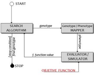
Figure 2.1: Interactions between elements of an evolutionary setup: edges represent input/output. In red: the objective function as an input for the evaluation stage, together with the phenotype (controller)

When it comes to automatic design of robots, there are many elements to take into consideration: a configurable or evolvable controller is needed, on which an algorithm that finds the best configuration for that con-troller is applied. The algorithm must be able to evaluate how good each configuration performs on the required task, for this purpose an ob-jective function is used. Sometimes a more convenient and/or compact representation of the controller’s evolvable parameters can be used in the evolutive process (genotype). A mapping can then be defined to obtain the controller corresponding to that representation (phenotype).

With all this elements in place we define an evolutionary setup (see Fig-ure 2.1). For each one of these (controller, algorithm, fitness function1_,

genotype-phenotype mapping) there are however many possible imple-mentations that will be explored in the following sections.

2.1.1

Evolvable Controllers

There are many controllers that can be evolved with an algorithm, some of them are usable only in the evolutionary robotics (ER) field, others

1_{“fitness function” usually refers to a type of objective function used in GAs but}

since here this distinction is not needed, this term will always refer to an objective function.

can be also designed manually. Among the most used, we can find:

• Artificial Neural Networks (ANN)

These are the most used evolvable controllers due to their fast con-vergence and the complexity of the tasks that can be learned. Al-gorithms have been developed that can train this kind of network in a very short time (e.g. NEAT algorithm in Stanley et al. [18]) that aren’t task-specific and can be used on many tasks (see Kohl and Miikkulainen [12]). The variable parameters in the evolution process are the weights of the edges, the thresholds of neurons and in some cases even the network topology. The downside of choos-ing ANNs is mainly the fact that once a solution is obtained, one doesn’t know how it internally works thus making impossible to test properties or doing any kind of analysis (except on very small networks) and can only be used as black-boxes.

• Programs (executable code)

Programs composed of executable instructions can also be used as evolvable controllers: once an instruction set has been defined, many algorithms can be used to search the space of all the possible programs of a given length. As an example in Busch et al. [3] a program evolved with a genetic algorithm is used to generate a walking loop on different robot morphologies.

• Finite State Automata (FSA)

Attempts on the evolution of FSAs have been done in Francesca et al. [6] with the main benefit of the solution being human-readable. Using an FSA means that one can easily combine primitive para-metric behaviours by considering them as states in the automations.

• Random Boolean Networks (RBN) This kind of networks have been used only recently as controllers in ER and since it’s the one on which this study will focus on, it will be explained in detail in section 3.

2.1.2

Fitness functions

A core element of the evolutionary cycle illustrated in figure 2.1 is the fit-ness function which once evaluated, discriminates the “good” controllers from the low performing ones. The training of a robot for a given task entirely depends on the formulation of the right fitness function that can select the most successful controllers without including task-specific

aspects that may introduce a bias in the process. A suggested classi-fication for fitness functions in ER is based on the degree of “a priori knowledge”(see Nelson et al. [14]) and from the most to the least task-dependent, can be summarized as follows:

• Training data fitness functions

These are the kind of fitness functions that measure errors on datasets containing example of task instances coupled with the ex-pected output. Using these functions means that the task is almost completely defined and the robot is not going to discover anything new, so they’re better suited for classification tasks or where the robot have to mimic the behaviour of a human.

• Behavioral fitness functions

Task-specific functions that measure how good the robot is doing by evaluating key sensing/acting reflexes useful for the task (e.g. in obstacle avoidance, a term that give an higher score to robots that turns when front proximity sensors are stimulated). These are often composed of many terms (one for each needed behaviour), combined in a weighted sum.

• Functional incremental fitness functions

Used in incremental evolution where simpler or primitive behaviors are learned first, and the evolutive path is assisted by the fitness function that change through the evolution until reaching the one that evaluates the complete task. These usually requires an a priori knowledge similar or lower than behavioral ones, but the course of evolution is restricted resulting in more trivial solutions and less novelty.

• Tailored fitness functions

The function measure the degree of completion of the task, thus re-quiring less knowledge about possible solutions, letting the robots free to explore all the possibilities (e.g. for a phototaxis behaviour, the distance separating the robot from the light should be mini-mized, as in Christensen and Dorigo [4]).

• Environmental incremental fitness functions

Similar to the functional incremental type but instead of adjusting the difficulty of the task, the robot is gradually moved to more complex environments.

• Competitive and co-competitive selection

This kind of selection force robots to compete for the same task (competitive) or for an opposite task (co-competitive, e.g. predator and prey) in the same environment so that even with a static simple fitness function, they are required to evolve more complex skill to beat the opponents.

• Aggregate fitness functions

These are high-level function that only measure success or failure of the required task so that almost no bias or restrictions are in-troduced in the evolution. Aggregate fitness functions require the minimum level of a priori knowledge but they’re also heavily af-fected by the bootstrapping problem (see Matteini [13]).

2.1.3

Search algorithms

Once an initial solution has been evaluated, we need to search for new ones in the space of all the possible controllers, that get better fitness function scores. Usually getting the optimal configuration is out of the question in this field2 _{due to the large size and low autocorrelation of the}

search field, hence many heuristic search methods are used.

The main block on which many search algorithms are built is the Stochas-tic Descent (SD) algorithm that works as follows: first a neighborhood function is defined on the search space, that assigns to each solution a set of close alternative configurations. Starting from an initial solution a random neighbor is evaluated, and if it gets a better score than the origi-nal configuration, we move to this one and pick another random neighbor to test, an so on. From a search field perspective, what this algorithm does is moving towards a local optimum and stopping there.

Many trajectory-based meta-heuristics are created from SD that mainly aim to prevent the algorithm from stopping in a local minimum in var-ious ways: accepting worsening steps (Random Iterative Improvement, Simulated Annealing), modifying the neighborhood structure (Variable Neighborhood Search) or scores (Dynamic Local Search), tracking the al-ready explored solutions (Tabu Search) or applying a perturbation to the solution and then start SD again (Iterated Local Search).

Another way to approach the search is by considering many candidate solutions at once and evolve them together exploiting their interactions; these are called population-based meta-heuristics. An example is PSO

2_{Actually, an optimal solution cannot even be defined in this context because the}

(Particle swarm optimization) where while new local optima are found, particles (that represent the current candidate solution swarm) are moved towards them hoping to find a good region of the search landscape. The Ant Colony Optimization algorithm makes another good example by us-ing an indirect interaction achieved depositus-ing pheromone in the envi-ronment toward which other solutions (ants) are attracted.

The most used class of population-based meta-heuristics are evolution-ary algorithms, inspired by the Darwinian evolution theory. These are based on three main operators applied to the population: a selec-tion process decides which soluselec-tions (genotypes) will be used to breed the next generation, then a combination of crossover (which recombine two or more different genotypes into new ones) and mutation (which is a random alteration of a genotype) operators is used to obtain the new genotypes.

2.1.4

Genotype-phenotype mapping

Many types of evolvable controllers can be expressed in a compact form that only includes their variable parameter values, creating a sort of DNA of a given configuration called genotype. In this form, the space of the possible solutions can be better explored and complex operator can be easily applied to a given configuration in a meaningful way (e.g. crossover operator in evolutionary algorithms). The possible encodings for a genotype, as suggested by Gen and Cheng [9] are:

• Binary encoding

• Real-Number encoding

• Integer or literal permutation encoding • General data structure encoding

A good encoding should also follows four properties that can be summa-rized as follows:

• Legality Any encoding (genotype) permutation corresponds to a solution (phenotype).

• Completeness Any solution has a corresponding encoding. • Lamarckian Property the meaning of a subset of the encoding

• Causality Small variations on the genotype space due to mutation imply small variations in the phenotype space.

2.2

The black box problem

Even if some attempts have been made in using controllers that once evolved are human-readable (Francesca et al. [6]), these often impose too many constraints to the evolution process, thus making them less likely to find a solution than more complex networks like ANNs or RBNs. When the evolution process is over, and we end up with a working prototype, we can evaluate its performance with an objective function or by visual validation, but no properties can be checked on complex networks and the only option is to use them as black-boxes which close up many real applications. For the same reasons it’s a fortiori hard to analyze their internal behavior, which can’t thus be modified to add for example man-ual extensions or corrections.

In chapter 3 we will explain the basics of boolean network robotics as an example of robot design based on a complex and evolvable network, while in chapter 4 a new methodology to analyze these networks will be proposed. This will be modeled on state-space trajectories already ob-tained through the evolution of RBN-controlled robots on three different tasks which can be easily analyzed

Chapter 3

Boolean Network Robotics

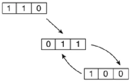
Boolean networks (BN) are composed of a set of N boolean variables that represent the networks nodes. To each node a boolean function is assigned, that is used to process values from all the other nodes to which its connected with an incoming edge and gives an output value that is then assigned to the node itself. In this thesis we will always refer to synchronous boolean networks, in which all the nodes are updated to-gether with a fixed frequency using as input the network state before the update. Even if the network model is very simple, BN can exhibit com-plex dynamics that can be visually observer through their trajectories (Figure 3.1).

Figure 3.1: example of a BN trajec-tory: states show the value of all net-work nodes while edges connect states to the possible future ones after the update.

One way to use BN in robotics as controllers is to map some of the network nodes to its sen-sors and actuators: sensen-sors val-ues will be processed by an input-encoding block that has as output a set of bits, each one assigned to a network node. These input nodes will not be updated by the network but only by the input-encoding block. In a similar way, some other nodes are encoded as input val-ues for the robot’s actuators by an output-encoding block (Fig-ure 3.2).

In the last years some work have been done on a particular type of BN: random boolean networks (RBNs). These are boolean networks where the functions that connects boolean variables are randomly generated. This can be easily achieved by fixing the number of input variables for each function to a constant value K and generating 2K _{boolean values}

that represent the truth table output for that function.

Figure 3.2: Schematic of the used coupling between BN an robot from Garattoni [7].

RBNs can show complex dynamics similar to the one obtained from other complex networks (e.g. ANNs) with the benefits of a finite state space of size 2N _{where N is the number of boolean variables.}

This kind of controllers can be evolved in various ways and studies have been carried out to find the most effective methodology(Amaducci [1]): the two easier ways to perform a mutation on the network are to either flip a bit in the truth table of a function, or to rewire the function input nodes. This last one has been proven to be ineffective so the networks used in this study were all evolved with the bit-flipping mutation. This kind of networks have been used only recently as controllers in ER showing good results on both simple tasks (e.g. Obstacle avoidance task) and memory-based tests (e.g. Sequence learning) with the only main dis-advantage of the I/O limitations: input from sensors needs an encoding step before being injected as boolean values in the network, and the same is true for outputs that are expressed as booleans and requires a map-ping to the actuators. This can be a problem if the task require complex I/O values or if you need to use analogical/continuous I/O since common binary encodings aren’t always effective.

Figure 3.3: The phototaxis / anti-phototaxis behaviour tested on a real e-puck robot. Above you can see the arena with the light and the e-puck moving toward it, a “clap” will make the robot turn around to run away from the light.

In Roli et al. [17] the effective-ness of RBNs used as robot con-trollers is shown, together with a methodology to automatically de-sign them based on stochastic local search techniques. This methodol-ogy is applied on a task that alter-nate an anti-phototaxis behaviour to a phototaxis one when a signal (“clap”) is perceived on a micro-phone equipped on the robot (the experimental settings can be seen in Figure 3.3). A simple stochas-tic descent is used to search in the space of all the possible truth ta-ble configurations by only flipping one bit of one table each time. An incremental approach is used for the objective function. Out of 30 runs of the design procedure, 4 robot controllers were successfully trained.

Vichi [19] shows instead the ca-pabilities of RBNs in the swarm

robotics field on a pattern recognition task: the swarm is placed on a floor and each robot can only sense the ground below itself and com-municate locally with the nearest robots. They should all turn led on when a given pattern on the ground is detected, and keep them all off otherwise. A first experimental section of the work is used to search for a good optimization algorithm for this class of tasks, then a series of test are performed. The results on the complete task are weak but the methodology is proven to work on simplified versions, and an in-depth analysis on the exchanged data is performed.

Bongard [2] uses RBNs for a different purpose: to evolve structural mod-ularity in robots controlled by complex networks. Starting from the fact that fully connected networks will be less and less viable for increasingly complex tasks, a procedure to automatically develop structural modu-larity is explained. Connections of 14-nodes RBNs are evolved (where a mutation consist on adding or removing one of them) to accomplish

an object-grasping task performed by a robotic arm with six degree of freedom. The results shows an emerged (and automatically designed) modularity in the networks that succeeded on the given task.

A first step into the search of FSA behaviours in RBN controllers is taken in Garattoni et al. [8] where the viability of using this kind of net-works as an intermediate design step in the synthesis of FSA is shown. The study is performed on two different tasks: a corridor navigation task involves the robot trying to reach the end of a corridor avoiding collisions with the walls, and a sequence recognition task in which as opposed to the first, memory is required. With evolution the RBNs are shown to move toward a compression of the state space with an usage of 100÷200 states against the potential 2N (N = number of nodes). Also looking at the frequencies with which different states are visited, the behaviour is shown to revolve around few states, which are connected to a cluster of other states in which the BN remains until a specific input is received. These are shown to be associated to with behavioral units of the robot and can thus be mapped to the states of a FSA obtaining simple readable behaviours that shows the viability of extracting FSA behaviours from trajectories of these networks in the state space.

The article is based on two previous RBN theses by Amaducci [1] and Garattoni [7]. Both works are constructed around the evolution of e-puck robots on three different tasks (phototaxis, obstacle avoidance, sequence learning) making use of RBN controllers and on the analysis of the final networks. By looking at both the RBN state space and the value of the objective function, the learning process is shown to be associated with a growth of the number of used states in the network (exploration phase), followed by a compression phase where the cardinality of the state space is reduced. The convergence speed of the proposed design process is also tested on different starting network conditions: ordered, critical and chaotic networks with different number of nodes.

In Amaducci [1] the focus is on the emergence of memory and on how this is connected to basins of attraction. The effect of different mutation techniques on memory is discussed, in particular the rewiring of boolean functions is compared to the flip of a bit in the truth tables.

A more in-depth analysis of convergence speed of the evolution process is performed in Garattoni [7] where the methodology is tested with differ-ent meta-heuristics (Stochastic Descdiffer-ent, Iterated Local Search, Variable Neighborhood Descent and Genetic algorithms).

FSAs that exploits Boolean network robotics as a convenient intermedi-ate step” has been hypothesized. This work aims to effectively complete this study by developing the step that allows an automatic extraction of the FSA behaviour from RBN’s state-space trajectories. Since this method will be based on state-space trajectories that can describe the dynamics of any time-discrete system with a limited state-space, it will be possible to apply it to study any other systems for which we can produce these trajectories.

Chapter 4

FSA behaviours extraction

method

In previous works (see chapter 3) attempts at analyzing RBN internal behaviour have been made using State Space Trajectories (SST). These trajectories are nothing more than a sequence of arrays of boolean values, each of which represents the state of all network variables in a give time step. Here we can talk about time steps because the previous works’ experiments are based on the synchronous update model for BNs and, since these have been carried out using the ARGoS(see Pinciroli et al. [16]) simulator, all the SSTs of the tasks analyzed in this study have been recorded and are already available.

Because of the limited number of nodes used by these networks, many re-peated frame sequences can be found in SSTs and a good way to increase their readability is to visualize them as FSAs: each network configuration found in the SST is mapped to a FSA state, and states corresponding to frames that appear consecutively in the SST are linked with a direc-tional edge. To make the diagram more readable some filtering has been already tested (see section 4.1), but most of the analysis were carried out manually.

The aim of this study is to develop an automatic and generic (task-independent) methodology to extract readable and functional FSA be-haviours from SSTs thus achieving 3 results: (1) enabling the use of RBNs as an intermediate step into the automatic design of FSA, (2) au-tomating and speeding up future RBN (and other systems) analysis, and (3) improving our understanding of RBN while developing the behaviour-extraction methodology.

network1 _{together with the list of the nodes used for I/O in the RBN.}

An unfiltered FSA diagram is initially created from SSTs as explained above and using this algorithm:

1 //inputs

2 List<SST> ssts;//A list of sst to be processed

3 //outputs

4 FSA behaviour;//The resulting fsa behaviour

5 //algorithm

6 behaviour.SetInitialState(ssts[0].GetFirstFrame()); 7 foreach(SST currentSST in ssts)

8 {

9 Frame lastFrame ← currentSST.CurrentFrame;

10 currentSST.Next();//go to the next frame

11 Frame currentFrame; 12 do 13 { 14 currentFrame ← currentSST.CurrentFrame; 15 if(!behaviour.ContainsState(currentFrame)) 16 { 17 behaviour.AddState(currentFrame); 18 } 19 20 behaviour.AddTransition(lastFrame → currentFrame) ; 21 lastFrame ← currentFrame; 22

23 }while(there are other frames) 24 }

Starting from this FSA a list of filters is applied sequentially until a compact and readable behaviour is obtained. Each filter is aimed to the correction of a specific problem in FSAs directly created from SSTs and only take as input the diagram to be filtered:

1 //inputs

2 FSA behaviour;

3 List<Filter> filters;//All the behavioural filters

4 //algorithm

5 foreach(Filter f in filters) 6 {

7 behaviour ← filter.ApplyTo(behaviour); 8 }

1_{Note that two or more SSTs can be combined together only if the network}

config-uration is exactly the same, which means the same truth tables and wirings together with the same initial node values.

In this work many SSTs have been studied and each of the filters that will be explained in the following sections is justified by an observed learning artifact: the more our understanding of this networks increases, the more we can raise the resulting behaviour’s quality.

4.1

Internal transients

Internal transients are the first pattern removed from the raw FSA ob-tained from SSTs, this technique was partially used in the previous works to reduce the numbers of states and make the resulting state machine a bit more readable.

Before going into how the algorithm to remove them works, we’ll have to agree on the concept of internal transient:

Def. 1. An interval of frames [Si, Si+k] from an SST is an Internal

transient of length k if all the I/O nodes from the frames in the interval [Si−1, Si+k] have the same values.

So this means that during this kind of transient, the only behaviour we’ll see is the one exhibited in the frame Sithat will be hold for k+1 time

steps, in other words all the transient can be removed without altering the behaviour itself. One may argue that internal transients can be explained as “waiting behaviours” and are thus not negligible but we shouldn’t think to the original RBN synchronous update as an input to the network since its just a technical detail of how these networks perform; if we need our BN to keep track of time, we should assign it to a sub-set of nodes as input. With that said, the algorithm to remove these transients is the following:

1 //inputs

2 FSA behaviour;

3 List<Filter> filters;//All the behavioural filters

4

5 //create IO mask

6 bool[] ioMask ← 0;

7 foreach(Filter f in filters) 8 {

9 ioMask ← ioMask or f.mask;//combine masks

10 } 11

12 //filter internal transients

13 foreach(State s in behaviour) 14 {

16 {

17 State destination ← t.DestinationState;

18 while((destination xor s) and ioMask = 0)//same IO

19 {

20 if(destination.TransitionCount > 1)

21 {

22 //if we found a branching state, we

are no longer in a trasitory

23 break; 24 } 25 destination ← destination.Transitions[0]. DestinationState; 26 } 27 s.RemoveTransition(t); 28 s.AddTransitionTo(destination); 29 } 30 }

31 //remove states from internal transients (that are now unreacheable)

32 behaviour.RemoveUnreacheableStates();

In the above pseudo-code, lines from 6 to 10 describes the creation of the IO mask: this is a binary mask of length equal to the number of nodes in the network that will have a bit set to 1 only if the corresponding node is an I/O node. This is used in line 18 with a bitwise and to mask out the other internal nodes and only compare I/O nodes.

4.1.1

Output flickering

Some outputs are known from the task to be purely reactive, which means that they won’t change by themselves without an external input. In a network that only relies on boolean variables even for I/O, output flickering is inevitable, but if we know for sure that a given output have to keep its value during an otherwise internal transient, we can filter out the noise by excluding it from the IO mask before executing the algorithm above (see section 5.2 for an example). Let’s say that a given input node Ni changes and the output node No starts to change many

values before the network reach an attractor. The algorithm will detect the change in Ni but since Nois excluded from the I/O mask, will behave

as it would for an internal transient, searching for a visible effect of that input. When the attractor is found, No will have its final (stable) value

and the algorithm will remove all the transient containing its unstable values.

4.2

Naming of edges and nodes

To increase diagrams readability some kind of naming for edges and nodes is needed. Of course, since the type of transducers is unknown2, the naming procedure should be driven by the user. This is done through I/O mapping tables that assign a name to each state of a given sensor or actuator (see 4.1). The output mapping tables are used to name the

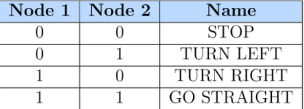
Node 1 Node 2 Name

0 0 STOP

0 1 TURN LEFT

1 0 TURN RIGHT

1 1 GO STRAIGHT

Table 4.1: An example of an output mapping table for the e-puck wheels’ motors: each motor is mapped to a network node (Node 1, Node 2). Each possible value combination of these nodes is associated to an output name that can then be used to describe each state composing a behaviour (e.g. a state where both nodes are active is a state where the robot goes straight).

states: they are accessed using the boolean values from the RBN state to be named. The edges naming is instead done comparing the input nodes from the two state that they connect: if a sensor state has changed, its input mapping table is accessed with the destination state values, and the resulting name is showed on the arch.

2_{Here we are only testing the procedure on simulated e-puck robots’ SST for which}

available sensors and actuators are well known. However abstracting from the type of robots on which RBNs are used keeps this study more generic.

Figure 4.1: Access to an output mapping in red, access to input mapping in green: here an xor is used to test for changes, if the result is > 0 the second value is used to access the table.

4.3

Initial transient

In all the studied SSTs, evolved boolean networks that are started with no inputs (or with default inputs) move along an initial transient that brings them to a standby attractor from which the actual behaviour starts. This can be justified by the fact that the initial network state is not evolved by the genetic algorithm and the network has to learn how to move itself into the starting configuration. This initial transient can be easily removed from the behaviour that gains in fact better performances. This is a simplification of the algorithm used to remove the initial transient:

1 //inputs

2 FSA behaviour; 3

4 //count the number of input edges for all states

5 Map<State→int> inputArchesCount;

6 foreach (State s in behaviour) 7 { 8 foreach (Transition t in s) 9 { 10 inputArchesCount[t.Destination]++; 11 } 12 } 13

14 //remove states until an attractor or branch is reached

15 State newInitialState ← InitialState;

16 while (

18 newEntryPoint.Transitions.Count = 1 19 ) 20 { 21 behaviour.RemoveState(newInitialState); 22 newInitialState ← newInitialState.Transitions[0]. Destination; 23 } 24

25 //add a more readable "START" state

26 State start ←new State("START");

27 behaviour.AddState(start);

28 behaviour.AddTransition(start → newInitialState); 29 behaviour.InitialState ← start;

4.4

Transients and Attractors Filter

One of the greatest limitations of RBNs used as controllers are the output capabilities that makes evolution hard on two fronts: on the one hand the output nodes number should be kept as low as possible to make the evolution process faster with a smaller search space, on the other hand many actuators works with analog input signals (e.g. e-puck wheel mo-tors) and using a few-bits binary encoding to pilot them means greatly underusing their potential and creating very “jerky” behaviours. This can of course be prevented by an appropriate output-encoding block, but from an SST point of view this could be taken into account by just replacing output node values with the actual sampled output values after the encoding step, we can thus abstract from the controller/robot cou-pling here. Looking at the trajectories of fully evolved RBNs, we can see that evolution try to overcome these problems by exploiting serializa-tion: when a given output value is not available, a transient emerge that “mix” the available values creating the needed one. An example of this type of adaptation can be found in section 5.1. Since this serialization effect can be also found in attractors3 _{the number of states used for the}

behaviour can get very high so a new filter will be applied to behaviours, which works with the following algorithm:

1 //inputs

2 FSA behaviour; 3 //outputs

4 FSA comprBehaviour; 5

3_{Attractors that includes more than one state give in fact a repeated chain of}

6 //count the number of input edges for all states

7 Map<State→int> inputArchesCount;

8 foreach (State s in behaviour) 9 { 10 foreach (Transition t in s) 11 { 12 inputArchesCount[t.Destination]++; 13 } 14 } 15

16 //create compressed attractors

17 foreach (State s in behaviour) 18 { 19 List<State> currentChain; 20 State currentState ← s; 21 22 while(currenState.HasDefaultTransition) 23 { 24 currentChain.Add(currentState);

25 //get the next state following the default

transition

26 State nextState ← currentState.DefaultTransition.

Destination;

27 if(currentChain.Contains(nextState))

28 //the chain looped back: attractor found

29 {

30 //compress the chain into a single−state

attractor

31 State[] aStates ← ExtractAttractorChain(

currentChain, nextState);

32 State attractor ← CompressAttractor(aStates

);

33 //save which states are from attractors

34 MarkStatesAsAttractor(aStates);

35 //add it to the new behaviour

36 comprBehaviour.AddState(attractor); 37 } 38 39 } 40 } 41 42 //isolate transients

43 Map<State→List<State>> transients;

44 foreach (State s in behaviour) 45 {

46 State curState ← s;

47 List<State> transient;

48 while(curState is not an attractor state)

50 if (inputArchesCount[curState] > 1)

51 //curState is reacheable by many states:

52 //end of this transient

53 break;

54 if (transients.Contains(curState))

55 //this links to another transient: merge them

56 { 57 transient.Append(transients[curState]); 58 transients.Remove(curState); 59 break; 60 } 61 transient.Add(curState); 62 if (states[curState].Transitions.Count != 1)

63 //branch (>1) or terminal state (0)

64 //this transient ends here

65 break;

66 //go to the next state on this transient

67 curState ← curState.Transitions[0].Destination;

68 }

69 transients[transient[0]] ← transient; 70 }

71

72 //create compressed transients

73 foreach(List<State> tr in transients) 74 {

75 //compress the chain into a single state

76 State comprTransitory ← CompressTransitory(tr);

77 //add it to the new behaviour

78 comprBehaviour.AddState(comprTransitory); 79 }

Basically, the FSA is firstly decomposed in transients and attractors that are then compressed into a single state, which describe the overall behaviour. This kind of approach can be used because the order in which these outputs are serialized don’t usually affect the final result for two reasons:

• these transients are almost all composed of two type of outputs randomly repeated many times

• RBN-evolved behaviour are usually very robust with many loop-backs that choose what to do based on the network current input state, so an approximation of this kind can be tolerated in most cases.

Since we should abstract from the output type, the serialized outputs are not really combined, but they are listed together with a number that

indicates the percentage of states in which that output appears. This process also increase readability by reducing the total number of states used in the FSA.

4.5

Fixed Output Chains

Another recurring pattern that can be found in extracted FSAs are fixed output chains (FOC). These state chains have no behavioral meaning and are the result of observing a robot behaviour through SSTs: since the network state is also composed of input nodes, input variations captured in consecutive frames are interpreted as transitions to new states, even if the network behaviour don’t change. Most of the evolved attractors are very robust and only react to a very limited number of inputs thus, from an SST point of view, an attractor is often followed by long chains of other transients and attractors which are all equivalent and with the same output of the first one. These states can therefore be removed without altering the behaviour and giving a more clear representation of the main attractors using this algorithm:

1 //inputs

2 FSA behaviour;

3 //isolate fixed output chains

4 Map<State→List<State>> fixedOutputChains;

5 foreach (State s in behaviour) 6 {

7 fixedOutputChains[s].AddState(s);

8 State nextState ← s;

9

10 while(

11 (transient or single−state attractor)

12 and

13 (the output is the same)

14 )

15 {

16 //get the first transition that brings to a new

state

17 State nextState ← s.getNextState();

18 //add the new state to the chain

19 if(fixedOutputChains.Contains(nextState))

20 {

21 //the two linked chains are merged

22 MergeChains(s, nextState);

23 break;

24 }

26 {

27 //add this state to the current chain

28 fixedOutputChains[s].AddState(nextState)

29 }

30 }

31 } 32

33 //replace chains with single−state attractors

34 foreach(List<State> chain in fixedOutputChains) 35 {

36 State compressedChain ← GenerateAttractor(chain);

37 behaviour.RemoveAllStates(chain); 38 behaviour.AddState(compressedChain); 39 }

To avoid removing previous input memorization behaviours, only iso-lated state chains are affected4_{. This algorithm will be applied twice}

to remove also chains that are generated in some rare configurations in the first pass: e.g. an attractor of size 1 generated by the first iteration becomes part of a fixed output chain removed by the second iteration.

4.5.1

Similar states

The FOC filter can also be used at another level: to approximate be-haviours. From a pragmatical point of view, this filter remove chains composed of single-state attractors and transients where the output is constant. If we relax the meaning of constant to similar we can exploit the above algorithm to merge states that produce similar behaviours by just changing the condition at line 13. A very simple definition of sim-ilarity will be used here, which aims to compress the behavioral states created by the transients and attractor filter (see section 4.4): two states will be considered similar if they exhibit the same outputs, ignoring per-centages.

4_{Isolated state chain refers to transients in which only the first state can be reached}

from external states (i.e. from states that are not part of the transient) and only the last state can have more than one transition to external states.

Chapter 5

Test cases

The methodology explained in the previous chapter will be tested on three diffent tasks for which a RBN controller has been evolved and SSTs are available. The first two tasks are from Amaducci [1] and Garattoni [7], namely obstacle avoidance and sequence learning, the last one is the phototaxis/anti-phototaxis composed behaviour explained in Roli et al. [17]. A visual comparison of the FSA before and after filtering will be made, then to test if the extracted behaviours actually works they will be implemented and tested in simulation using ARGoS 2.

5.1

Obstacle avoidance

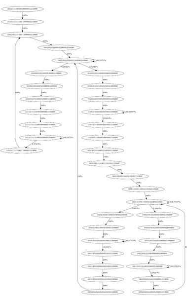
This is a simple task commonly used to test evolutionary robotics tech-niques. In this case the robot was placed at one end of a corridor with an orientation that varies from one trial to another. The robot goal was to reach the other end of the corridor avoiding wall collisions, and many networks with good performance were evolved but with a basic conversion of their SSTs into an FSA one would get the diagram shown in Figure 5.1, which is neither readable nor usable and requires further manual analysis.

With this result in mind lets now look at the diagram extracted with the proposed methodology (see Figure 5.2): we can easily identify where the behaviour starts and the main features of this diagram. A first attractor is used to move straight along the corridor, but when a wall is identi-fied on the left (FRONT/LEFT arch) or on the right (FRONT/RIGHT arch), the robot will first turn respectively right or left and then moves straight until the wall is not detected anymore (NO OBSTACLES edges).

Figure 5.1: Obstacle avoidance diagram converted directly from SSTs: even decoding the state meaning in terms of I/O don’t make it readable, since 38 states are too much for this simple behaviour.

Figure 5.2: Extracted obstacle avoidance behaviour: the number of states dropped to 5 + 1(start) and named edges makes this version more readable and usable.

The two states with a composed behaviour are created by the Tran-sients/Attractors filter (see section4.4): TURN LEFT or TURN RIGHT primitives provide a too sharp turn to be used by themselves that would make the robot bounce from a wall to the other, thus the evolution focus on solutions that serialize the above primitives with the GO STRAIGHT one, softening the turn.

5.2

Sequence learning

Sequence learning was originally a good task to test RBN ability to de-velop memory: this task requires the robot to run through a corridor with colored bands on the floor that can be read using e-puck ground sensors. Given a correct sequence of colors, the robot should memorize the previ-ous readings and turn on its leds when a correct sequence appear. The colors used for the floor are black, gray and white. The correct sequence for this task was an alternation of black and gray (starting with black) with white used as separator between each value. The SST converted to FSA for can be seen in Figure 5.3 and are again of little help. Again, good results were achieved but with the problem expressed in section 4.1.1: flickering. The leds required some RBN update cycles to stabilize during which they randomly light up. This behaviour can be easely ana-lyzed looking at Figure 5.4. Since we know that leds should only turn on or off in response to an input value, we can remove them from the I/O

mask, extracting an optimal behaviour for this task (see Figure 5.5).

Figure 5.4: Behaviour extracted using the proposed methodology, for the sequence learning task. Led state change during many transients.

Figure 5.5: Extracted sequence learning behaviour with flickering removed on leds.

5.3

Phototaxis/anti-phototaxis

Figure 5.6: Phototaxis/Anti-phototaxis behaviour extracted with the f.o.c filter: the chain is replaced with a single attractor.

This composed task consists in a phototaxis behaviour, that changes to an anti-phototaxis one after the robot hears a clap. The robot was trained on the phototaxis task first, and then on the complete behaviour. if we try to represent its behaviour without any inference, we would see the graph in Figure 5.8 that again, is not readable. The results using the proposed method are shown in Figure 5.6 where the two behaviours can be easely identified, separated by the “clap” transition: as imposed by the objective function used the phototaxis behaviour is robust to errors in orientation while the clap makes causes the robot to turn 180 degrees and move forward without checking if the correct direction is preserved through time. After the clap, while the robot turns in the opposite direction, the light sensors changes many values that are ignored by the RBN: this results on a fixed output chain artifact explained in section 4.5 and visible (with the FOC filter disabled) in Figure 5.7. By enabling the filter, the fixed output chain is removed making the anti-phototaxis behaviour more clear (Figure 5.6).

Figure 5.7: Phototaxis/Anti-phototaxis behaviour extracted without the f.o.c filter: a chain of states with the same output can be seen after the “clap”.

Figure 5.8: Phototaxis/anti-phototaxis diagram converted directly from SSTs.

5.4

Filtered Behaviours validation

The increase in readability of filtered behaviours is easely visible, but they should also be validated. To do that, the FSAs extracted in the previous sections will be implemented on the same simulator to test how they perform, compared to the original RBNs from which they’re extracted. For the obstacle avoidance test, the FSA in Figure 5.2 will be used. The corridor with obstacles can be seen in Figure 5.9: the robot should reach

the end of the corridor avoiding obstacles. The results with this FSA are very poor, with the robot that only successfully avoid the first obstacle or starts to run in circles(see Figure 5.10).

Figure 5.9: Simulation of the obstacle avoidance test: the robot in blue on the right should move along the corridor avoiding the obstacles in red.

This can be easely explained by overfitting: we are trying to extract a complete behaviour from a single successful SST that only contains the trajectory of the network for a single scenario. This can only bring to a failure because of the many different situations that the robot can encounter in a generic run. If we only think about the input mapping of the robot, we have a 4-bit mapping for the proximity sensors that results in 24 _{= 16 possible configurations that should be tested for each state in}

which the RBN can be found, this means that one run contains by far to few frames to completely define the task.

The behaviour extraction methodology can also combine many runs of the same robot to improve the results, but even combining 6 different runs (with different initial robot orientations) was not enough to extract a working behaviour. So the main problem here is that we are using SSTs extracted from trials performed by the robot, while to obtain a functional behaviour we should collect SSTs from a complete (or almost complete) I/O test. This is something that is likely to be feasible on a RBN because of the limited state space, but its not guaranteed to work: while we observe a behaviour through SSTs we can’t discern the actual network problems from the one caused by an insufficient amount of data. The unfiltered FSA obtained from the six runs looks like a collection of examples that could both mean that (a) we don’t have enough SSTs or (b) the network itself is affected by overfitting.

Figure 5.10: Trajectory obtained from the extracted behaviour in the ob-stacle avoidance task. Once the first obob-stacle is reached the robot starts to turn left, but since in the SSTs from which this behaviour is extracted this would eventually result in the activation of only the back/right sensors, the robot know how to behave only in that scenario, while in the other variations it never stops turning left.

To prove these concepts the sequence learning extracted FSA(see Fig-ure 5.5) has also been tested. Here the robot has only to go straight and the behaviour ends up ignoring the proximity sensors so we should only look to the ground sensors used to sense the sequence color. This is en-coded in two bit but with only three possible configurations that stands for the three possible ground colors: black, grey and white. Since white is used as a separator, the network can work correctly by only remembering the previous non-white color which can be grey or black only.

Figure 5.11: Simulation of the sequence learning test: the robot in blue on the right should move along the corridor signaling a correct sequence on the ground by turning leds on each time it runs over a color. In this case only the last black strip is out of the sequence, and leds should be kept off while crossing it.

Assuming that separators are always placed correctly, we ends up with only 2 · 3 = 6 scenarios (2 previous colors and 3 possible inputs) which is pretty low. In this case since we are extracting the behaviour from 10 different runs, we should have enough data to get a behaviour

that is not only readable, but also usable on a robot. The test arena can be seen in Figure 5.11 were the robot should turn the leds on if a color in the correct sequence is detected while moving along the corridor. The robot performed the task correctly in all the test runs as expected, giving better results than the original RBN due to the flickering reduction filter applied during the behaviour extraction.

Chapter 6

Behaviour evolution analysis

Since with the proposed methodology is now easy to analyze RBNs be-haviours, we can exploit it to process many SSTs instead of focusing on one, opening up some possibilities for new analysis. In this chapter, tra-jectories from many generations of the same network will be compared to better understand how evolution works from a behavioral point of view. For this purpose, we’ll look at the obstacle avoidance task, for which SSTs from all the generations have been collected. The evolution process is composed of a total of 2000 generations, so we are sampling 7 of them, taken among the generations that introduced the greatest improvements:

Generation Number Score (to be minimized)

0 5.09744 128 0.736159 206 0.617284 226 0.531898 317 0.488747 608 0.337947 Final Generation 0.270777

The behaviours extracted from these generations are illustrate in Fig-ure 6.1, 6.3, 6.2, 6.4, 6.5, 6.6.

Figure 6.1: In its initial form at generation 0, the behaviour is composed of a single attractor that makes the e-puck moving forward.

Figure 6.2: In generation 206 a compression phase has already simplified the behaviour in his two main branches. The attractor that makes the robot turn left when an obstacle is sensed on the right appeared.

Looking at these behaviours we can confirm the hypothesis of the existence of exploration and exploitation phases [1] [7] in RBNs evo-lution: in generation 128 (Figure 6.3) we are in the exploration phase where the evolution is looking for new solutions, while in the following generations state compression and behaviour polishing is performed (ex-ploitation phase) while the network itself converges to a local optimum.

Figure 6.3: Generation 128: the first two events of an obstacle on the left or right are already visible but the behaviour is still blurry. An obstacle on the right can bring the FSA to a terminal attractor that implements an undefined behaviour.

Figure 6.4: Generation 226, a wrong attractor is removed with obstacles on the left.

Figure 6.6: Wrong behaviour removed from right branch in generation 608.

The improvements on behaviours during the evolution process seem to be non-destructive and fine enough when needed. Of course this is only a single example and we cannot prove anything here, but the evolu-tion process brings to a local optimum even from an FSA point of view showing the stability of the proposed behaviour-extraction methodology. Another interesting way to use this kind of analysis is during the net-work evolution: since behaviour extraction have a low computational cost, one could use features extracted from FSA analyzed in this section to improve the objective function and drive evolution in the right direc-tion. Complexity can be in fact correlated to fitness[11] and if we think to SSTs as a data-stream, Crutchfield [5] suggests that its complexity can be measured by features of the machine used to generate it, that in our case is represented by the corresponding extracted FSA behaviour.

Chapter 7

Generality of the method

Up to this point, the behaviour extraction method has been only referring to SSTs of boolean network: this is because of the availability of already documented experiments and tests that speeded up all the analyses car-ried out in this paper. However the method is actually based on SSTs themselves, meaning that any link to boolean networks can be easily weakened to make it relevant for any discrete-time system with a limited state-space as already outlined is chapter 3. Starting from this point we can make a few considerations on which part of this methodology is generic, which isn’t and how to enable its application to other systems. In Figure 7.1 we can see the behaviour extraction method placed in a process that would work for many systems, even if not discrete-time. After simulating the system and recording its dynamics, we can encode them into SSTs directly if the system is already discrete-time and with limited state space, or sample and quantize them otherwise. This means that applications of this method to continuous-time systems like ANNs are possible.

Concerning the proposed methodology, since the only analyzed SSTs comes from RBNs, overfitting is likely to be present in some filters that solve problems which may or may not affect other systems.

Figure 7.1: A proposed process that would enable to use the method on a generic system. Squares represents processing blocks, while edges are data flows.

Chapter 8

Implementation

Figure 8.1: The GUI of the .Net applicative implementing the behaviour extraction methodology: the current FSA is visible at the center, the blue bar on top is used to adjust the amount of filtering. Moving it to the right increase the number of applied filters creating a more approximated but cleaner behaviour. The list on the top/right show the I/O mappings that can be edited, saved, loaded from file.

To make tests easier and the proposed methodology available to other researchers, a simple implementation has been created for the .NET plat-form. This allows the user to import one or more SSTs files and process them while viewing the resulting FSA behaviour real-time. I/O map-pings can be also configured through the application as well as saved in a binary file. Once the desired behaviour is obtained, this can also be ex-ported as a graphviz dot file, image or even a compilable C++ controller for the ARGoS simulator. The GUI can be seen in Figure 8.1, while I/O mappings can be created as seen in Figure 8.2.

Figure 8.2: Creation of a new mapping: Clicking “Add” (1) will make a new window pop up, write the list of the node to which the sensor/actuator is mapped (2) and click next (3) to add the mapping. The mapping windows will become visible to let you modify the namings (4), specify if its a sensor or an actuator and enable the flickering filter on this node. Closing the window (5) will confirm any editing on this mapping.

Chapter 9

Conclusions

A methodology for the extraction of FSA behaviours from the state-space trajectories of RBN has been successfully created. The results on the readability side are good enough to work with all the three proposed tasks, even when small amount of data is available. In section 5.4 these behaviour has been also validated in ARGoS, showing that the required amount of SSTs for the behaviour to work is proportional to the number of possible inputs and states in which the robot could find itself and thus only the sequence learning FSA have given good results when tested. In chapter 6 analysis have been made on SSTs from networks spanning different generations making visible how RBNs evolution alternates ex-ploring phases to compression phases and how this kind of analysis could be used on-line to drive the evolution process. The extracted behaviours are thus both readable and usable, but we shouldn’t misunderstand their meaning: these FSA are not extracted from the RBN itself but from SSTs that results from the interaction of the RBN with a given environ-ment. This means that the resulting FSA shows how the robot behave in the target environment but makes no assumptions on how it will work in different situations. Of course since the proposed methodology can work on many distinct SSTs at the same time (combining them in a single behaviour), all the situations meaningful to the tasks can be taken into account, but as showed in section 5.4 this could not be enough. A formal methodology for extracting meaningful SSTs for a given task should help overcoming this problem and is suggested as a future work.

Finally in chapter 8 an implementation has been given to the method that will hopefully allow other researchers to speed up the analysis pro-cess of RBNs.

An important evolutionary problem emerged during SSTs analysis is that sometimes behaviour could be dependent on the frequency of the clock

used for the synchronous update: in the extracted behaviours this emerge in the form of transitions with no guard. These are to be understood as transitions triggered after a time equals to the the one between two up-dates of the source RBN, but as explained in section 4.1 this event should not be taken into consideration in the evaluation phase during evolution. As a proposed solution and future work, we could think to an evolu-tionary process that also vary the update frequency to make the network robust to it (e.g. running the same trial many time with different update frequencies), such an approach would also make this behaviour-extraction methodology more reliable.

In this study RBNs has been chosen as an example of complex networks because of the previous available analysis on their internal behaviour and the fact that SSTs can be easely obtained by encoding their binary state. However as suggester in chapter 7 this methodology have the potential to be applied to other types of networks such as ANNs by quantizing the output of neurons.

Bibliography

[1] M. Amaducci. Design of boolean network robots for dynamics tasks. Seconda Facolt`a di Ingegneria, Universit`a di Bologna, 2011.

[2] J. C. Bongard. Spontaneous evolution of structural modularity in robot neural network controllers: artificial life/robotics/evolvable hardware. In Proceedings of the 13th annual conference on Genetic and evolutionary computation, pages 251–258. ACM, 2011.

[3] J. Busch, J. Ziegler, C. Aue, A. Ross, D. Sawitzki, and W. Banzhaf. Automatic generation of control programs for walking robots us-ing genetic programmus-ing. Genetic Programmus-ing, Lecture Notes in Computer Science Volume 2278, 2002, pp 258-267, 2002.

[4] A. L. Christensen and M. Dorigo. Evolving an integrated phototaxis and hole-avoidance behavior for a swarm-bot. IRIDIA, Universit´e Libre de Bruxelles, Belgium, 2006.

[5] J. P. Crutchfield. The calculi of emergence: computation, dynamics and induction. Physica D: Nonlinear Phenomena, 75(1):11–54, 1994.

[6] G. Francesca, M. Brambilla, A. Brutschy, V. Trianni, and M. Birat-tari. Automode: A novel approach to the automatic design of control software for robot swarms. Springer Science+Business Media New York, 2014.

[7] L. Garattoni. Advanced stochastic local search methods for auto-matic design of boolean network robots. Seconda Facolt`a di Ingeg-neria, Universit`a di Bologna, 2011.

[8] L. Garattoni, A. Roli, M. Amaducci, C. Pinciroli, and M. Birattari. Boolean network robotics as an intermediate step in the synthesis of finite state machines for robot control. In P. Li`o, O. Miglino, G. Nicosia, S. Nolfi, and M. Pavone, editors, Advances in Artificial Life, ECAL 2013, pages 372–378. The MIT Press, 2013.

[9] M. Gen and R. Cheng. Genetic algorithms and engineering opti-mization. John Wiley & Sons, 2000.

[10] G. S. Hornby. Automated antenna design with evolutionary algo-rithms. University of California Santa Cruz, 2006.

[11] N. J. Joshi, G. Tononi, and C. Koch. The minimal complexity of adapting agents increases with fitness. PLoS computational biology, 9(7):e1003111, 2013.

[12] N. Kohl and R. Miikkulainen. An integrated neuroevolutionary ap-proach to reactive control and high-level strategy. IEEE TRANSAC-TIONS ON EVOLUTIONARY COMPUTATION, VOL. 16, NO. 4, 2012.

[13] M. Matteini. An overview on automatic design of robot controllers for complex tasks. Seconda Facolt`a di Ingegneria, Universit`a di Bologna, 2014.

[14] A. L. Nelson, G. J. Barlow, and L. Doitsidis. Fitness functions in evolutionary robotics: A survey and analysis. 2008.

[15] S. Nolfi and D. Floreano. Evolutionary robotics, 2000.

[16] C. Pinciroli, V. Trianni, R. O Grady, G. Pini, A. Brutschy, M. Bram-billa, N. Mathews, E. Ferrante, G. Di Caro, F. Ducatelle, M. Birat-tari, L. Gambardella, and M. Dorigo. Argos: a modular, parallel, multi-engine simulator for multi-robot systems. Swarm Intelligence, 6(4):271–295, 2012. ISSN 1935-3812. doi: 10.1007/s11721-012-0072-5. URL http://dx.doi.org/10.1007/s11721-012-0072-10.1007/s11721-012-0072-5.

[17] A. Roli, M. Manfroni, C. Pinciroli, and M. Birattari. On the design of Boolean network robots. In C. Di Chio, S. Cagnoni, C. Cotta, M. Ebner, A. Ek´art, A. Esparcia-Alc´azar, J. Merelo, F. Neri, M. Preuss, H. Richter, J. Togelius, and G. Yannakakis, editors, Applications of Evolutionary Computation, volume 6624 of Lecture Notes in Computer Science, pages 43–52. Springer, Heidel-berg, Germany, 2011.

[18] K. O. Stanley, B. D. Bryant, and R. Miikkulainen. Real-time neu-roevolution in the nero video game. Department of Computer Sci-ences University of Texas at Austin, TX 78712 USA, 2005.

[19] D. Vichi. On the design of a boolean-network robot swarm, collective recognition of ground patterns. 2012.