Synthetic DNA as a novel data storage solution for digital images.

SCUOLA DI INGEGNERIA E ARCHITETTURA Corso di Laurea Magistrale in Ingegneria Informatica

SYNTHETIC DNA AS A NOVEL DATA

STORAGE SOLUTION FOR DIGITAL

IMAGES

Relatore:

Prof.ssa

SERENA MORIGI

Correlatori:

Prof.

MARC ANTONINI

Dot.ssa

EVA GIL SAN ANTONIO

Presentata da:

MATTIA PIRETTI

Abstract 3

Introduction 4

1 State of the Art 7

1.1 Works on DNA data storage . . . 7

1.2 Related works of image inpainting . . . 9

2 Workflow for DNA data storage 12 2.1 Compression . . . 12

2.1.1 Computation of Damage Detection parameters . . . 14

2.2 Encoding and Formatting . . . 15

2.2.1 Preventing sequencing noise during Encoding . . . 17

2.2.2 Barcoding process . . . 18

2.2.3 Silhouette clustering for Double Representation . . . 23

2.3 Biological procedures . . . 25

2.3.1 Synthesis, Amplification and Sequencing . . . 27

2.3.2 Types and effects of sequencing errors . . . 28

2.4 Consensus establishment . . . 31

2.4.1 Barcode correction . . . 32

2.4.2 Outlier detection . . . 33

2.5 Deformatting and Decoding . . . 35

2.6 Post-processing . . . 35

2.6.1 Automatic Damage Detection . . . 37

2.6.2 Wavelet inpainting . . . 41

3 Experimental results 45 3.1 Analysis of the expected damage . . . 47

3.2 Experiments with realistic Nanopore noise . . . 50

3.3 Experiments with worst-case noise . . . 53

3.4 Numerical experiment . . . 57

4 Conclusions 60

Thanks 62

During the digital revolution there has been an explosion in the amount of data produced by humanity. The capacity of conventional storage devices has been struggling to keep up with this aggressive growth, highlighting the need for new means to store digital information, especially cold data. In this dissertations we will build upon the work done by the I3S MediaCoding team on utilizing DNA as a novel storage medium, thanks to its incredibly high information density and effectively infinite shelf life. We will expand on their previous works and adapt them to operate on the Nanopore MinION sequencer, by increasing the noise resistance during the decoding process, and adding a post-processing step to repair the damage caused by the sequencing noise.

Keywords: DNA, DNA data storage, long-term storage, Biologically con-strained encoding solution, Image coding, Biological information theory, Ro-bust encoding, Outlier detection, Damage detection, Image inpainting, Blind inpainting, Inpainting in the wavelet domain

The amount of data produced and consumed by humanity has been steadily increasing for years, with an estimated 90% of all data available on the internet having been produced over the last two years. Most of this data is due to an explosion in multimedia content. However, much of this new content is also very rarely accessed, with close to 80% being effectively “cold” data. Nonetheless, this content must be stored and maintained for security and legal compliance. The sheer volume of data produced forces large companies to invest into entire data centers to house the conventional storage mediums, incurring in exorbitant costs to build all the security, power supply and environmental infrastructure surrounding one such endeavor. Additionally, this investment risks being just the tip of the iceberg. The mean time between failures of traditional storage solutions, like Hard Disk Drives and magnetic tapes, is measured in years, a couple of decades at most. This means that every few years the data must be migrated to a new set of devices to ensure reliability, adding a sizable recurring cost to the whole enterprise.

A novel alternative, that has become of great interest over the past few years [46], is to use DNA as a storage medium. DNA is a complex organic molecule, constituted by four building blocks, commonly referred to as nucleotides (nt): Adenine (A), Thymine (T), Cytosine (C), and Guanine (G). As the support for heredity used by living organisms,

DNA possesses several properties that could make it a very effective medium to hold human generated data. Firstly, it can be an extremely dense medium, information wise, with a single gram of DNA being theoretically capable of storing up to 455 Exabytes of data under optimal conditions. This extreme data density is due to both its three-dimensional structure and quaternary encoding base. Secondly, it can retain information

for incredibly long periods of time, persisting for centuries and even millennia in a still readable state.

To use DNA as a storage medium is a very involved process, but it can be schematized as follows. Firstly, the digital data has to be encoded into a quaternary schema using the four DNA symbols A, T, C and G. Then, the DNA string needs to be synthesized. As the synthesis process is error free as long as the sequences produced are less than 300nt in length, the encoded data must first be split into smaller chunks. These are referred to as “oligos” and are formatted in a way that includes Headers to carry the meta-information needed to reconstruct the original encoded sequence, by aligning the oligos in the right order. The oligos are then finally synthesized and stored in a hermetically sealed capsule. This prevents contact with damaging agents and ensures their durability.

When the information needs to be retrieved, the capsule can be opened and the oligos read via specific machines called sequencers. This step is one of the sticking points for the whole process, as the sequencing tends to be a very error prone step. However, the sequencing error can be minimized (but for now not eliminated) by abiding to some biological constraints. These include limiting the total length of the synthesized DNA strands, as well as avoiding excessive repetitions of nucleotides and patterns in the oligos. The encoding algorithm must then be able to respect these restrictions, as is the case for the code previously proposed in [54]. Then, to complete the decoding, the sequenced oligos are amplified through a process called Polymerase Chain Reaction , filtered, and finally used to reconstruct and decode the originally encoded data.

In addition to the noisiness of the sequencing, the high cost of DNA synthesis and sequencing has remained one of the main drawbacks to biological data storage. However, over the last few years the nanopore sequencing technology [47], along with its portability, affordability and speed in data production has been revitalizing the idea of DNA storage. There are, of course, drawbacks. The faster sequencing times come with a much higher error rate when compared to other slower, more expensive, but more reliable sequencers.

To deal with the increased noise, abiding by the biological restrictions of the process is fundamental, but not necessarily sufficient. A host of works (see for example [50] and [56]) have focused on tackling this higher error rate by relying on error correction techniques

that increase the redundancy of the encoding. This however incurs into an increase of the encoding cost. The approach developed during the internship with the I3S MediaCoding [64] team marries a biologically constrained encoding process with noise resilience and post-processing techniques.

This work was originally developed during a year-long Erasmus mobility period, hosted by the Sophia Antipolis Polytechnique. The work was conducted as a six months internship at the CNRS’s I3S Labs in Sophia Antipolis, as part of the MediaCoding team, and as continuation of a previous month-long project exploring the barcoding process. In this dissertation we will cover the work done during these six months.

We will provide the reader with a background on the current state of the art in chapter 1, regarding the current works on DNA data storage as well as most common inpainting techniques utilized for occlusion removal. In chapter 2 We will then proceed to outline a comprehensive workflow that allows for reliable encoding, storage, decoding, and repair of digital images onto synthetic DNA. This workflow, built upon the previous work done by the I3S MediaCoding team, will be geared toward operating on the Nanopore MinION[55], a much more portable and cheap sequencer than the classical Illumina[42] machine. During the exposition of this workflow we will highlight and discuss the novel additions brought by us during the internship, along with the effects of these contributions and the circumstances that necessitated them. For reference, these contributions will be covered in subsection 2.1.1, subsection 2.2.3, section 2.4 and section 2.6.

Lastly, in chapter 3 we will show the results of the encoding, decoding and post-processing workflow on two different images at different levels of sequencing noise. After that, in chapter 4, we will offer our view of the proposed work and possible future improvements and extensions.

State of the Art

In this chapter we will provide a brief overview of the current literature. We will start by quickly analyzing the evolution of DNA data storage over the years in section 1.1, from its first implementations in the early 2010s [29] to the previous works done by the I3S MediaCoding team, that we will be expanding upon. This is done to provide the reader with a background into the current state of the art of DNA encoding, as well as the sticking points of common approaches. In section 1.2 we will then perform a more expansive analysis of the literature regarding image inpainting. We will focus mostly on the pros and cons of different inpainting approaches, rather than their evolution over time, as we want to provide a background on the various families of inpainting algorithms. We will refer back to this analysis when discussing how to repair the damage caused by the sequencing noise and our choice of algorithm for the Wavelet Inpaiting in section 2.6.

1.1

Works on DNA data storage

There have been several proposed implementations to encode data, especially media files, onto DNA. The first attempt was done in [29], which also provided an analysis of the main cause for biological errors. Later studies focused on guaranteeing noise resistance, as the error rate of the process became a sticking point for all works concerning the practicalities of DNA data storage. In [34] and [44] the problem was approached by

Figure 1: Storage capacity of modern magnetic tapes compared to DNA[29].

splitting the encoded data into overlapping segments, so that each fragment is represented multiple times. This technique, however, is not scalable and adds excessive redundancy. Other approaches include the use of Reed-Solomon code to treat erroneous sequences and guarantee the recovery of missing oligos [41], and performing forward error correction by utilizing more than one dictionary during encoding, so as to encode each symbol with more than one nucleotide sequence [45]. Lastly, [58] proposed a method that integrates Huffman coding in the encoding, in order to store quantized images onto DNA. This work also introduced the idea of utilizing post-processing techniques to correct the discoloration in the reconstructed image.

These approaches, however, are all based on introducing redundancy, which increase the global cost of the synthesis, rather than consider the input’s characteristics. Other works have focused on introducing compression to DNA coding which, coupled with avoiding unnecessary redundancy, can help minimize the synthesis cost. The team’s previous works [51],[54] focused on one such approach. Additionally, in [57], was proposed a novel DNA encoding algorithm for quantized images, capable of respecting the biological constraints, while providing a new way to map the Vector Quantization (VQ) indexes to DNA codewords so as to minimize the impact of errors in the decoded image. This adds resistance to noise without having to rely entirely on error correction.

focused on the Illumina sequencer due to its higher accuracy. The work we are introducing here, instead, is geared toward Nanopore sequencing, in order to speed up the process and reduce its cost. To do so we will extend the work presented in [57] by applying the novel mapping algorithm to the DWT decomposition of an image, and adding an extra post-processing step, based on the inpainting algorithm described in [18], so as to reduce the visual artifacting in the reconstructed image.

1.2

Related works of image inpainting

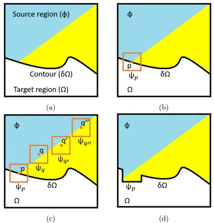
Image inpainting is an approach aimed at repairing damage (or at removing unwanted objects) from images in a way that is seamless to the human eye. What sets image inpainting apart from other restoration techniques like haze-removal is that there is virtually no information to be gained from inside the damaged area. An inpainting algorithm must operate on information taken either from the undamaged parts of the image or, at most, from the contour between these and the target (damaged) area.

There are many families of inpainting algorithms and, similarly, a lot of different classifications are possible. A first macro division can be seen between structural inpainting techniques, textural inpainting methods and hybrid approaches [40]. The first type of approach focuses on the structure of the image, generally the isophote lines and the edges of shapes in the undamaged part of the image. These are then propagated into the damaged area via mathematical means. Texture-based approaches instead focus more on the replication, propagation, or synthesis of textures in the image. Hybrid approaches take aspects of both inpainting families.

A second, more detailed, classification could divide these macro families based on their algorithmic approaches. We would then have Partial Derivative Equations (PDE) based approaches, semi-automatic inpainting algorithms, texture synthesis methods, model/template based methods and a catchall family of hybrid algorithms that exhibit specific characteristics [38],[30]. We will focus more on a couple of these approaches, namely PDE, texture synthesis and exemplar-based approaches, and cover the others more briefly. The goal here is to highlight what are the strengths and weaknesses of

each approach, rather than present a comprehensive comparative review of the different inpainting techniques.

PDE approaches rely on purely mathematical inpainting algorithms, inspired by the partial differential equations that describe the flow of heat in the physical world. The idea can be traced back to [11], where it was proposed a method through which the information is propagated from the intact area into the damaged one, by following the isophote lines crossing the boundary between the two. Already from this first approach one can see the strength and weaknesses of PDE methods, as they have remained pretty much the same since then. While these techniques are very good and efficient at covering narrow damages, they cannot effectively reconstruct textures (see [25]). As such the blurring effect they create becomes very noticeable when trying to cover up large damages. Several other works have improved over PDE methods, with the introduction of second order derivatives in [12] and high order PDE in [21], but the limitations of these approaches remain the same.

Semi-automatic inpainting approaches require, as the name suggests, user interaction for the process to complete. For example in [20] the user is prompted to sketch the contour of the objects in the occluded area, before a texture synthesis algorithm applies the inpainting. This is in addition to the detection of the damaged area, that in virtually all the approaches mentioned in this chapter is assumed to be done outside of the algorithm itself, presumably by the user. As already stated, we require a way to automate the entire post-processing, and as such these methods are not what we are looking for.

Texture synthesis algorithms and exemplar-based approaches are often considered separately, but for our purposes they fall under the same umbrella. Both focus on the use of pixel color and texture to repair damaged areas without causing blur, and both have similar pros and cons. Texture synthesis approaches take a small sample of true texture and try to replicate it. This can be done pixel by pixels, starting from the edges of the occluded area [10], or more efficiently by considering whole blocks of pixels at a time [13]. Even with this optimization, the texture generation approach can be computationally expensive and still struggle with more complex textures. Exemplar-based methods side-step the texture generation problem by sampling and copying existing color

values from a specified source. This is commonly done from the undamaged parts of the image [15], but other solutions rely on entire databases of images similar to the damaged one [23]. Nonetheless, all these methods tend to present similar behaviors: they perform well when covering large, regular occlusions, but struggle with repairing complex or irregular textures. Additionally, they risk causing artifacting due to the order in which the textures are copied from the source to the damaged area. In this vein, Criminisi’s algorithm [18] merits a special mention, as it is an exemplar-based approach that tries to account for and prevent this drawback.

The hybrid approaches are generally intended as methods that rely on both structure and texture information, usually gained by a decomposition of the image. From this point of view [18] could be classified as hybrid, due to the way its priority-based filling order is computed. Most of the works in this category try to split the image into a structure and a texture component [14],[16] and inpaint them separately before merging the results. Two sub-families merit mention here. The first are wavelet-based approaches. While they are an important background, they relate less to our problem than one might hope, as we will show in subsection 2.3.2. These inpainting algorithms [28],[32] rely on Wavelet Transform as a decomposition tool, to split the image into structure and texture information. While the approach is interesting, it does not match our situation. The second sub-family of hybrid algorithms is that of machine-learning based approaches. It is debatable whether this should be considered a family in and of itself, or whether the work of the convolution layers matches the definition of “decomposing” the image into structure and texture information. In any case, this is an approach that is becoming more prominent lately, relying on both convolution [48],[53] and deep [31] neural networks. These methods can be very good at handling blind-inpainting, where the mask of the damage is not given a priori. This would be an excellent match for our needs, and the approaches certainly merit further investigation in subsequent works. However, all machine learning approaches require a large amount of data that we did not have easy access to, as the pre-trained layers commonly used for these approaches were prepared over much different images and visual distortions than the ones we had to contend with.

Workflow for DNA data storage

In this chapter we will first cover all the steps of the encoding and decoding process to familiarize the reader with the structure of the work. Additionally, we will investigate in more detail and provide some background for processes that appear often throughout the workflows, or that are especially relevant to the project as a whole.

Several steps are required to encode an image onto DNA, and to subsequently decode it correctly. The main steps are five, and can be seen exemplified in Figure 2. The innovations brought by this work add three additional main steps and can be seen exemplified in Figure 3. In the resulting workflow in addition to the five that are from the original implementation, an outlier detection step is added to the consensus establishment phase, and two new steps comprise a post-processing phase after the decoding is complete. We will now cover each step in detail.

2.1

Compression

Firstly, a Discrete Wavelet Transform (DWT) is performed [9]. This takes advantage of the spatial redundancies in the image to decompose it into subbands, by passing through a series of low and high-pass filters. These are sub-images with width and height equal to 2−𝑁 _{times those of the original image, where N is referred to as the “level” of the}

Figure 2: Previous workflow, presented and utilized in both [51] and [54].

Figure 3: Novel proposed workflow. Additional steps shown in red, and presented in subsection 2.1.1, subsection 2.4.2, and section 2.6.

DWT. The HH, HL and LH subbands carry local variations in pixel color, meaning they generally represent the details of the image, while the bulk of the information is carried by the LL subband. An example of DWT applied to the image we will be utilizing during the rest of this work can be seen in Figure 4. From here until the end of the decoding, we will be working exclusively on this decomposition, rather than on the entire image.

Figure 4: 2 level Discrete Wavelet Transform. Original image on the left, greyscale of the wavelet subbands on the right.

After the decomposition, each result-ing subband is quantized independently from the others with a Vector Quantiza-tion (VQ) algorithm [4]. To further ensure optimal compression, a bit allocation [7] algorithm is employed to provide the best quantization codebooks for each subband, in order to maximize the encoded bits per nucleotide. These two processes (DWT and

VQ) comprise the compression step.

2.1.1

Computation of Damage Detection parameters

After the compression step we introduce the first contribution of this work that expands the workflows already built in [51] and [54].

The damage detection step, that will be described in details in subsection 2.6.1, depends on a series of parameters. The most obvious of these are the two thresholds that determine whether a pixel is considered anomalous or not, but the definition of “neighborhood” for a given pixel is also going to influence the behavior of the algorithm. There are essentially two ways of determining these values: either the user can input them by hand, or an algorithm can be used to try and determine them. As automation of the damage detection was one of our main goals, we opted for the second option.

Normally, this would mean analyzing the noisy subbands obtained after the DNA decoding. The obvious drawback would be that deriving the information from a corrupted image might give erroneous results, causing us to set the thresholds to values that would cause too many false positives or, more likely, too many false negatives. However, we are in the unique position of having access to the ground truth, the undamaged image as it was encoded before synthesis and sequencing, because we control the entire workflow.

We decided to exploit this by inserting a very small additional step after the compres-sion. Here we define the neighborhoods for each subband and then analyze the image in the same way we would during the post-processing. At the end of this analysis we will have compiled a list of the values (difference from pixel’s neighborhood and variance within neighborhood) that would be computed during steps one and two of the damage detection process. We can then compute what are the acceptable thresholds from these lists, either by setting them to the highest value or to a lower one and accepting a certain number of false positives.

This parameter computation can be customized to the single subband. For example, the easiest way to do this is to accept more false positives in larger and less meaningful subbands, were loss of details is less problematic than distracting visual distortion.

Another way would be to modulate the shape and size of the neighborhoods based on those of the quantization vectors used for each specific subbands.

2.2

Encoding and Formatting

After the compression step (and the parameter computation step added by this work), the quantized subbands are to be encoded into quaternary code. To do this we first use the encoding algorithm proposed in [51] to create codebooks. This is done by merging predefined symbols into codewords. The symbols are selected from two dictionaries:

𝐷1 = 𝐴𝑇 , 𝐴𝐶, 𝐴𝐺, 𝑇 𝐴, 𝑇𝐶, 𝑇 𝐺, 𝐶 𝐴, 𝐶𝑇 , 𝐺 𝐴, 𝐺𝑇 𝐷2 = 𝐴, 𝑇 , 𝐶, 𝐺

Concretely, this means that we construct sequences of even length 𝐿 by concatenating

𝐿

2 symbols from the first dictionary 𝐷1, and sequences of odd length by adding a single

symbol from the second dictionary 𝐷2 at the end. So, for example, we can construct all the codewords of six nucleotides by computing all the permutations of three elements from 𝐷1 (𝐴𝑇 − 𝐴𝐶 − 𝐴𝐺, 𝐴𝑇 − 𝐴𝐶 − 𝑇 𝐴, 𝑒𝑡𝑐.), and the ones of seven nucleotides by adding one element from 𝐷2 at the end (𝐴𝑇 − 𝐴𝐶 − 𝐴𝐺 − 𝐴, 𝐴𝑇 − 𝐴𝐶 − 𝐴𝐺 − 𝑇, 𝑒𝑡𝑐.). The symbols that comprise these two dictionaries have been specifically chosen so that their concatenation always leads to "viable" words, meaning they abide by the restrictions indicated in subsection 2.2.1. Since the resulting codewords will be permutations of elements from the two dictionaries, this helps making the encoding more robust to the sequencing noise, without adding redundancy or overhead, as the words that would be more prone to misdecoding are discarded. Additionally, this algorithm is capable of encoding any type of input, rather than just binary.

After all the codewords have been constructed, the mapping binding these to the numerical values in the subbands is performed. This is done by the method originally presented in [5], that was expanded upon in [57]. The fundamental idea is to map the input vectors obtained from the Vector Quantization algorithm to the codewords generated by the coding algorithm. However, we also want to execute the binding in a

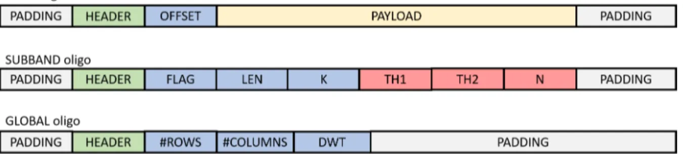
Figure 5: Formatting schema for the three oligo types. Oligo identifiers in green, metadata used during decoding in blue, metadata used during post-processing in red, and encoded information in yellow.

way that can minimize the impact of errors on the quaternary sequence. To do this, we map vectors that are close to each other, in terms of Euclidean distance, to codewords that are similarly close to one another, here in the context of Hamming distances. This means that, in case of a small distortion due to sequencing errors, erroneous words will still have a small Hamming distance from the correct ones, reducing the visual distortion that the errors cause in the reconstructed image. Again, this adds robustness against the sequencing noise without having to introduce costly redundancy in the encoding process.

As we will mention in section 2.3, the DNA synthesis process is effectively error free for short strands, in our case shorter than 250-300nt [65]. As such, the last process we need to undergo in this step is cutting into chunks of the appropriate size the encoded subbands that we just generated with the mapping and encoding algorithm. This also implies the necessity to add to each of these oligos some form of metadata, to indicate the position of the specific oligo in the input image. Not only that, we also need to similarly encode metadata related not just to the single oligo, but to the encoding process itself, as this information will be needed during the decoding. The end result is akin to the classical approach used for data packets that are to be transmitted over a network: a division of a large amount of information into smaller packets, each carrying one or more Header fields and replicated several times for robustness. The specific formatting schema we used can be seen in Figure 5.

As was the case in [51] and [54] we opted for a formatting schema revolving around three distinct types of oligos. The Global (G) oligo carries information concerning the

entire image, specifically its size and the levels of DWT used during encoding. A single Subband (S) oligo for each subband encodes the information concerning its encoding. In this case the VQ parameters: type (FLAG) and size (LEN) of the vectors used as well as the length of the codewords (K); and the information needed by the post-processing workflow: the threshold values (TH1 and TH2) and the size of the neighborhood (N) for the damage detection algorithm. Data (D) type oligos are carrying the actual information (PAYLOAD) as well as a field to identify the position of their Payload in the original data (OFFSET). Finally, all three oligo types have an identifying field (HEADER) that discriminates their type, and eventually the subband and level of DWT they belong to, to allow for their correct decoding. All oligo types also have some padding at the beginning and end as a concession to the distribution of the sequencing noise. This facet will be covered in more details in subsection 2.3.3 and subsection 2.3.2, but the necessity here is to try and preserve the Headers and metadata fields as much as possible, by protecting them with disposable DNA. Additionally, we protect the most important fields (especially the Header and Offsets fields) by relying on barcodes. These will be explored in more details in subsection 2.2.2, but they can be considered a type of self-repairing inline encoding. They are codewords specially chosen so that even in the presence of errors (up to a certain threshold) a correction algorithm is able to recover the original sequences from the noisy ones, without having to introduce any additional information other than the quaternary string itself.

2.2.1

Preventing sequencing noise during Encoding

We will cover the sequencing in more details in subsection 2.3.1, but for now we simply have to acknowledge that it is an extremely noisy process. While this noisiness cannot be completely avoided, it can be reduced if some biological restrictions are observed during the encoding process. Specifically, we must ensure that our DNA strands have the following features:

• No homopolymers over a certain length. A homopolymer is a repetition of the same nucleotide. The specific length varies between sequencer but can be assumed to be between a maximum of 3 and 6 nucleotides, meaning that ideally the same

nucleotide should not appear more than three times in a row in the final oligos. • The percentage of CG content should be lower or at most equal to that of AT

content.

• There should be no pattern repetition in the oligos.

The first two points are relatively easy to ensure, and the Single Representation (SR) encoding algorithm presented in [51] can guarantee that the oligos we create respect these restrictions. The third restriction is more complex to observe and has to be taken into account during the mapping.

To do this we can employ a technique called Double Representation (DR). This is an encoding method in which we build a codebook that is twice as large as the one that would be needed for traditional, SR, encoding. In SR, when a value needs to be encoded it is mapped to a single codeword, in DR it is instead mapped to one of two codewords chosen at random. This significantly reduces the repetitions of patterns in the Payloads of the oligos. This is especially true for the case of VQ-based compression, in which several adjacent indexes could be the same (for example, when encoding the background of an image, or large patches of solid color). In this work we decided to not test this approach and simply rely on SR, but the infrastructure needed to adapt the advanced encoding from [57] to use DR is already in place, including the codebook clustering algorithm described in subsection 2.2.3.

2.2.2

Barcoding process

As we already mention in subsection 2.2.1, it is possible to reduce the noisiness of the sequencing process by abiding to some biological restrictions. This, coupled with the redundancy added by the PCR amplification (covered further on is section 2.3), can be considered acceptable for the preservation of the data itself. It is not, however, sufficient protection for the metadata. Especially considering the findings of [43], we must protect the most important fields of the oligo further. While padding helps, we conducted several tests where crucial information (for example the Offset of the D oligos)

was simply encoded as we would any other data, and the resulting loss of oligos was unacceptable. As such we referred back to barcoding [33], a technique that the team had already relied on in previous works.

The use of barcodes to protect sensitive parts of the DNA encoding is not new and has been explored in several other studies over the years, see [24], [33], and [52] for some examples. The idea is to create a set of codewords with a high enough distance between them, so that in the case of an error we can correctly identify which codeword was the original one. In our case the codewords were constructed via the same algorithm we use for the encoding, guaranteeing that the barcodes themselves respect the biological constraints of the sequencing process.

For constructing the barcode sets from these codebooks We are using a greedy heuristic algorithm based on the work in [33] and shown in algorithm 1. Due to its greedy nature, this algorithm does not guarantee finding the maximal barcode set for a given codebook. It is much more efficient than an exhaustive search over the same set, as the generation of barcode sets is a very computationally expensive process. Given a codebook 𝐶∗ = 𝑐₁, 𝑐₂, . . . , 𝑐_𝑁 and the expected error tolerance 𝜇 the set construction procedure is as follows:

• Set 𝑆 = 1, create a first barcode set 𝐵𝑆 and add the first codeword 𝑐1of the codebook

𝐶∗ to it.

• Foreach codeword 𝑐𝑘 with 𝑘 = 1, 2, . . . , 𝐾 do the following:

– Check the distance between all the codewords in each barcode set 𝐵𝑖 with 𝑖 =

1, 2, .., 𝑆.

– If the distance between all codewords in a barcode set 𝐵𝑖 is bigger than

𝑑_𝑚𝑖𝑛 =2 × 𝜇 + 1, add 𝑐_𝑘 to the set 𝐵_𝑖 and move to the next codeword 𝑐_(𝑘+1). – If this condition was not met for any existing barcode set then set 𝑆 = 𝑆 + 1,

create a new barcode set 𝐵𝑆 and add the codeword 𝑐𝑘 to it.

Another way to see the problem is to consider the computation of the barcode set as the identification of the maximum independent set over a graph, where the vertices are

Algorithm 1: Barcode sets construction. Input:

𝐶 = (𝑐₁, 𝑐₂, . . . , 𝑐_𝑁) : codebook 𝜇: expected error tolerance. Output:

𝐵= (𝐵₁, 𝐵₂, . . . , 𝐵_𝑆) :barcode sets with error tolerance 𝜇. 𝑆← 1; 𝐵(𝑆) ← {𝑐₁}

𝑑_𝑚𝑖𝑛 =2 × 𝜇 + 1 for 𝑖 ← 1 to 𝑁 do

𝑓 𝑙 𝑎𝑔 ← false for 𝑘 ← 1 to 𝑆 do

𝑑_𝐵 ← mindistance between 𝑐_𝑖 and all the codewords 𝑐_𝐵 ∈ 𝐵_𝑘 if 𝑑𝐵 ≥ 𝑑𝑚𝑖𝑛 then 𝐵(𝑘) ← 𝐵(𝑘) + 𝑐_𝑖 𝑓 𝑙 𝑎𝑔 ← true break end end if ! 𝑓 𝑙𝑎𝑔 then 𝑆← 𝑆 + 1 𝐵(𝑆) ← {𝑐𝑖} end end

the words in the codebook 𝐶∗ _{and the edges connect the vertices that have distance lower}

than 𝑑𝑚𝑖𝑛. As this is a traditionally NP-hard problem, a non-greedy algorithm would

incur into an unsustainable computational overhead very quickly.

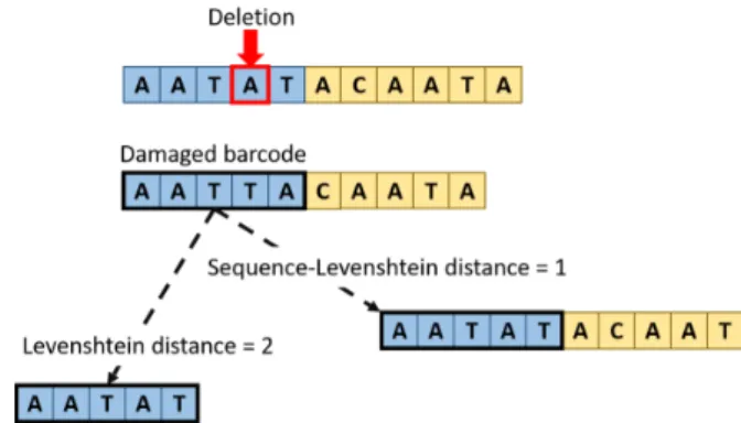
A quick aside is necessary regarding the distance that is used when constructing the barcode sets. Until now we did not go into any specifics, but it is worth it to dig a little bit deeper into this detail. For the entire of the barcoding process, both the assignment and the reconstruction, we consider as metric the Sequence-Levenshtein distance that is presented in [33]. An example of the difference between this and the classical Levenshtein distance [1] can be seen in Figure 6. In short, both distance metrics measure the number of steps needed to go from one string to another. The main difference is that classical Levenshtein counts each added, removed or changed letter (or nucleotide, in our case) as a distance of one, and sums these elemental steps to obtain the minimum total distance.

Figure 6: Example of difference between Leven-shtein and Sequence-LevenLeven-shtein distance.

In the context of DNA however, this is insufficient. Specifically, in the case of deletions, the first nucleotide from the rest of the DNA strand will appear at the end of the barcode. This is the shifting we previously mentioned, that makes Indels so hard to deal with. This means that the now noisy barcode will have a Levenshtein distance of two from the original one (one for the deleted nucleotide and one for the nucleotide that was inserted at the end from the rest of the oligo).

To remedy this, in [33] was introduced a new distance metric called Sequence-Levenshtein, as an extension of the classical Levenshtein distance, in which adding nucleotides at the end of a word does not increase the distance. The effect is twofold. On one hand this allows us to utilize it in the construction of barcode sets that can ensure recovery from deletions, on the other it also means that the classical Levenshtein distance is an upper bound of the Sequence-Levenshtein distance, resulting in closer words and

barcode sets of reduced size. This last detail can become an obstacle and forces a sort of “ballooning” in the codeword length for the barcodes when either a high error tolerance is needed (as it is for the identifying Header fields), or when the data to protect can have many different values (as it happens with the Offset of D oligos, that can reach well into the hundreds).

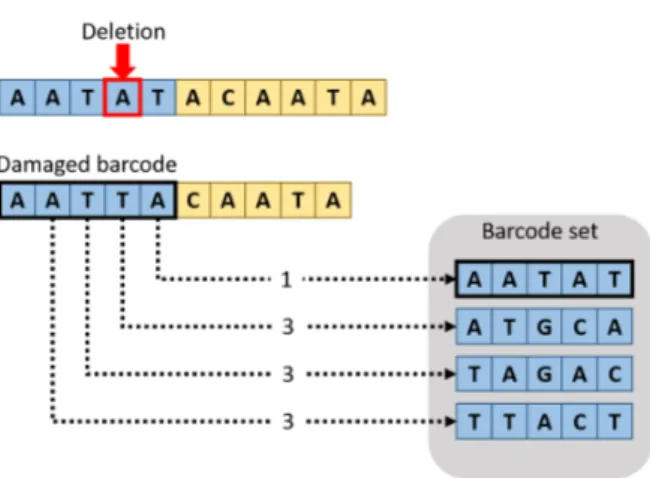
In Figure 7 we can see an example of the correction process. Let us suppose that a certain information, for example the Offset of the D oligos, has been encoded with the barcode set on the right. If the field containing the information suffers an error, in this case a Deletion, we can recover the information by comparing the resulting (damaged) barcode with the intact ones in the set. We can see that the damaged barcode (AATTA) does not appear in the set. This is because the barcode set was built to be resistant to one error, meaning each word has a distance of at least three from one another. As such, during the decoding we can clearly see that an error has occurred and attempt to repair it. This is done by comparing the erroneous barcode to each of the original ones and picking as correct the one that is closest.

Figure 7: Example of how a barcode can be recovered.

Of course, this does not guarantee that the value will be correctly recovered. If the number of errors is higher than the toler-ance of the specific barcode set, the noisy barcode could be unrecoverable (meaning it has a distance higher than the tolerance from every barcode in the set) or, even worse, it could be recovered erroneously to the wrong barcode. In the first case the barcode and whatever information it was carrying is lost, but the assumption is that the added redundancy from the PCR is sufficient to compensate for the loss. The

second case can be the source of potentially more impactful, and Byzantine, visual distortions in the reconstructed image. The erroneous correction of the Offsets in the D oligos is a big part of why we introduced an outlier detection step before the consensus,

in order to prune away oligos with Byzantine Headers that could poison the consensus for the oligo they were erroneously identified as.

2.2.3

Silhouette clustering for Double Representation

In subsection 2.2.1 we introduced the concept of Double Representation, an evolution of the classical encoding schema utilized in [54] that could reduce the amount of pattern repetitions in the formatted oligos. This method is very interesting, but cannot be directly applied to the advanced encoding presented in [57]. This is because the DR operates by selecting one of two random codewords to map to the numerical values during encoding. This stochastic selection obviously conflicts with the idea behind the DeMarca encoding, that tries to match close numerical values to close codewords to reduce the visual distortion caused by erroneous decoding. To try and reconcile these two encoding techniques, we developed in this work an ad-hoc clustering algorithm that given a codebook can split it into clusters based on the similarity between the codewords. This could allow us to map a value to one of two random codewords, while still guaranteeing that the values close to the number being encoded would be mapped to other codewords close to at least one of the randomly chosen ones.

Clustering as a whole is well treaded problem, that has been at the forefront of data-analysis for years if not decades [3],[49],[67]. The general idea is to classify a set of points, or objects, based on their position relative to each other. In most cases this is applied to unsupervised machine learning models, where the task is to group together unlabeled points to gleam some insight on the underlying structure of the data that is being analyzed. In our case, we have a slightly different problem. We know precisely how many clusters there must be in our data, the problem is finding which points belong to which cluster. This in and of itself is not uncommon, k-means clustering [2] is a very well-known method to separate a data-set into a given number of clusters. The problem with using a traditional k-means method, is that we also have a constraint on the exact number of points that must be in each cluster, as our mapping expects precise cluster sizes. While there is some work investigating versions of k-means clustering that account for underlying constraints of the data-set [68], adapting this approach to our needs was

deemed too costly.

As such we steered ourselves toward building a quick ad-hoc clustering algorithm based on the Silhouette Coefficient (SC), shown as pseudo-code in algorithm 2. Originally proposed in [6], Silhouettes are a metric used to validate and interpret clustering results. The SC (sometimes referred to as Silhouettes Index) is a tweak of this technique presented in [8], and still used in some modern applications [66]. The SC is a measure, varying between 1 and -1, that is calculated for every point, or object, in the data-set. The value of the coefficient indicates how appropriate is the assignment of an object to its current cluster, with 1 being a perfect assignment and -1 being the worst possible one. It is calculated by considering the average distance of each point from every other point in the cluster it is assigned to and comparing it to the average distance from all the other clusters. If the point is closer to the other points in its cluster it will have a positive coefficient. If it is closer to another cluster, the coefficient will be negative. Even from this quick definition, it can be inferred that the SC can be an expensive metric to employ, given that it requires the computation of the average distance with every point in the data-set, for all points. As our clustering needs were for very small sets (rarely above 1000 words) this overhead was considered negligible.

The way our algorithm works is as follows:

• First, compute the adjacency matrix for the entire codeword set. This is done to speed up the 𝑆𝐶 computation process.

• Assign to the set a random clustering, of course respecting the constraints on number and size of the clusters. This is done to introduce entropy in the data-set and eliminate any pattern that may be present in the original ordering of the codebook. • Repeat the following steps until the Silhouettes of the clusters stops meaningfully

improving, or a maximum number of steps has been reached:

– Compute the 𝑆𝐶 for all codewords in the set. Additionally, keep a list 𝑃 of

the preferred clusters for each codeword. This can be done during the 𝑆𝐶 computation with no additional overhead.

– Select a codeword 𝑐𝑖 at random from the ones with 𝑆𝐶 ≤ 0. This stochastic

approach, rather than choosing for example the codeword with the minimum 𝑆𝐶, is done both to avoid tottering issues and hopefully help push past eventual local minimum.

– Select the codeword 𝑐𝑗 with the lowest 𝑆𝐶 in cluster 𝑃(𝑐𝑖). Ideally the

coefficient of this second word will be negative, but it is possible that it might be close to or above 0.

– Switch the two codewords.

– Compute the improvement and move to the next iteration.

In this way the total Silhouette Coefficient should generally be increasing, as at each step we are assigning a word to its preferred clusters, while simultaneously removing from that cluster a second word that either would fit better elsewhere, or was on the edge between two clusters. If it does not, it means we have reached a plateau, or we are having tottering between a handful of points. In these cases, the algorithm terminates. Testing of the algorithm showed it to be reasonably performant on the codebooks we employed it on, up to 4000-10000 words. Eventually, it was decided to move forward with the noise simulation and post-processing testing described in chapter 3 without the use of Double Representation, to avoid muddling the results of the experiments, meaning this algorithm does not appear in the final work. But should a future work wish to use both DR and DeMarca encoding, especially in the case of a wet experiment, this might be a good way to join them together.

2.3

Biological procedures

The biological procedures step covers the “wet” parts of the process, that revolve around actual physical DNA. We will be covering them very briefly in subsection 2.3.1, as DNA synthesis and PCR exude from the scope of our work. In subsection 2.3.1 we will cover the differences between two types of sequencers, the Illumina (used by most older works regarding DNA data storage) and the Nanopore (whose behaviour we will be

Algorithm 2: Silhouette Coefficient clustering. Input: 𝐶 = {𝑐₁, 𝑐₂, . . . , 𝑐_𝑁} : codebook to cluster 𝐾: number of clusters 𝑀 : cardinality of clusters Output:

𝐶 𝐿= {𝐶 𝐿₁, 𝐶 𝐿₂, . . . , 𝐶 𝐿_𝐾} : clustering of the codebook 𝐶 𝐿← random clustering {𝐶 𝐿₁, 𝐶 𝐿₂, . . . , 𝐶 𝐿𝐾} 𝑆𝐶 = {𝑆𝐶_𝑐 1, 𝑆𝐶𝑐₂, . . . , 𝑆𝐶𝑐𝑁} ← {−1, −1, . . . , −1} ( 𝑆𝐶, 𝑆𝐶𝑖 𝑚 𝑝𝑟 𝑜 𝑣, 𝑃 )← computeSilhouetteCoefficients(C,SC,CL) while 𝑆𝐶𝑖 𝑚 𝑝𝑟 𝑜 𝑣 >0 do 𝑐_𝑖 ← random 𝑐_𝑖 ∈ 𝐶, with 𝑆𝐶 ≤ 0 𝐶 𝐿𝑖= {𝑐1, 𝑐2, . . . , 𝑐𝑖, . . . , 𝑐𝑀} : cluster containing 𝑐𝑖 𝐶 𝐿𝑗 = {𝑐1, 𝑐2, . . . , 𝑐𝑀} : preferred cluster 𝑃(𝑐𝑖)

𝑐_𝑗 ← codeword ∈ 𝐶 𝐿_𝑗 with min 𝑆𝐶 (𝑐_𝑗) 𝐶 𝐿_𝑖← 𝐶 𝐿_𝑖− {𝑐_𝑖} + {𝑐_𝑗} 𝐶 𝐿𝑗 ← 𝐶 𝐿𝑗− {𝑐𝑗} + {𝑐𝑖} ( 𝑆𝐶, 𝑆𝐶𝑖 𝑚 𝑝𝑟 𝑜 𝑣, 𝑃 )← computeSilhouetteCoefficients(C,SC,CL) Function computeSilhouetteCoefficients: Input: 𝐶= (𝑐₁, 𝑐₂, . . . , 𝑐𝑁) : codebook 𝑆𝐶 = (𝑆𝐶_𝑐

1, 𝑆𝐶𝑐₂, . . . , 𝑆𝐶𝑐𝑁) : Silhouette Coefficient for each codeword in 𝐶

𝐶 𝐿= (𝐶 𝐿₁, 𝐶 𝐿₂, . . . , 𝐶 𝐿𝐾) : current clustering Output: 𝑆𝐶0 = (𝑆𝐶0 𝑐₁, 𝑆𝐶 0 𝑐₂, . . . , 𝑆𝐶 0

𝑐𝑁) : new Silhouette Coefficient for each codeword in 𝐶

𝑆𝐶𝑖 𝑚 𝑝𝑟 𝑜 𝑣 : improvement of SC

𝑃= (𝑃𝑐₁, 𝑃𝑐₂, . . . , 𝑃𝑐𝑁) : preferred clusters of each codeword in 𝐶

𝑆𝐶_{𝑖 𝑚 𝑝𝑟 𝑜 𝑣} ← 0; for 𝑖 ← 1 to #𝐶 do 𝑐𝑖 = 𝐶 (𝑖) 𝐶 𝐿𝑖 = {𝑐1, 𝑐2, . . . , 𝑐𝑖, . . . , 𝑐𝑀} : cluster containing 𝑐𝑖 𝑎(𝑖) ← 1 #𝐶 𝐿𝑖−1 Í 𝑐𝑗∈𝐶 𝐿𝑖, 𝑗≠𝑖 𝑑𝑖 𝑠𝑡(𝑐_𝑖, 𝑐_𝑗) 𝑏(𝑖) ← min𝑘_≠𝑖 1 #𝐶 𝐿𝑘 Í 𝑐0 𝑗∈𝐶 𝐿𝑘 𝑑𝑖 𝑠𝑡(𝑐𝑖, 𝑐 0 𝑗)

𝑃(𝑐𝑖) ← cluster 𝐶 𝐿𝑘 with min average distance to 𝑐𝑖

𝑆𝐶0(𝑐_𝑖) ←          1 − 𝑎𝑖 𝑏𝑖 , if 𝑎_𝑖 < 𝑏_𝑖 0, if 𝑎𝑖 = 𝑏𝑖 𝑏𝑖 𝑎𝑖 − 1, if 𝑎 𝑖 > 𝑏𝑖 𝑆𝐶𝑖 𝑚 𝑝𝑟 𝑜 𝑣 ← 𝑆𝐶𝑖 𝑚 𝑝𝑟 𝑜 𝑣 + 𝑆𝐶 0_(𝑐 𝑖) − 𝑆𝐶 (𝑐𝑖)

simulating in this work). Lastly in subsection 2.3.2 and subsection 2.3.3 we will cover the incidence and types of sequencing errors that arise when using the Nanopore sequencer. Once the encoding is complete, the digital oligos are synthesized into biological DNA. As stated before, we can ensure that this process remains error free as long as we only construct synthetic DNA strands that are relatively short, in the 250-300nt range. The synthesized DNA can then be stored in hermetically sealed capsule. This is done to minimize the damage that DNA can incur in and is effectively the last step in the encoding workflow.

The decoding workflow begins with the recovery of these hermetic capsules and the extraction of the encoded DNA. This is then subjected to a process called Polymerase Chain Reaction, or PCR amplification. This is a precursor to the sequencing process, and is used to add redundancy to the oligos, by creating many copies of each one. While the process is not error free, the incidence of this noise is minimal compared to the effect of the sequencing of the oligos. As such, it is a very effective way to add a lot of redundancy to the process, as the amplification can result in several hundreds or even thousands of copies of each oligo being produced, without incurring in the exorbitant cost that such a level of redundancy would imply if it was achieved before the synthesis.

The sequencing, often referred to simply as the “reading” of the oligos, is the process with which the biological DNA strands are scanned and translated into a digital quaternary representation. This is done by machines called sequencers. As stated in the introduction, most of the work on DNA encoding, including the teams own work in [54], has been done on the Illumina sequencer [42]. While the initial large presence in the literature was due to it being among the first of the Next Generation Sequencers (NGS) [26], its staying power is a testament to the accuracy and effectiveness of the machine. The drawbacks of the Illumina sequencer are the natural flip-side of its strengths. The machine is very large, and the sequencing process is cumbersome, slow, and very expensive.

(a) Illumina sequencer.

(b) Nanopore MinION.

The Oxford Nanopore sequencer, especially its Min-ION version [47], are an up-and-comer of the sequencing scene. It is much cheaper, faster, and more portable than the Illumina and other classical NGS machines. Examples of both these sequencers in action can be seen in Figure 8b and Figure 8a. The main challenge keeping the Nanopore technology from more widespread adop-tion is the high error rate, especially when compared with the Illumina sequencer.

As the focus of this work was partly developing an encoding and decoding workflow that could be viable for use on the Nanopore MinION, understanding the types of errors that the sequencing could incur in was a top priority. Several studies have been conducted in this sense [43],[55].

2.3.2

Types and effects of sequencing errors

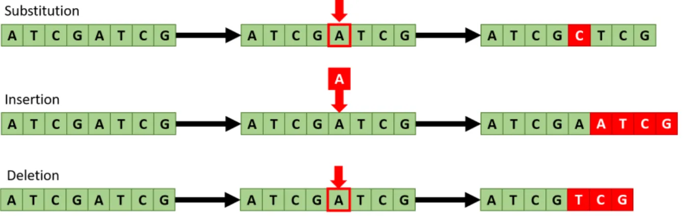
There are three types of errors that can be observed during the sequencing: Substi-tutions, Insertions and Deletions. In Substitutions a nucleotide is read erroneously, for example an Adenine (A) nucleotide is interpreted by the machine as being a Thymine (T). This obviously does not affect the order or values of the other nucleotides in the sequence. Insertions and Deletions, on the other hand, end up affecting all the nucleotides in the sequence that follow the error. The names are quite self-explanatory, a Deletion occurs when the sequencer “skips” a nucleotide during the reading, while an Insertion happens when a nucleotide that was not present in the original strand is erroneously added by the sequencer. Visual examples of all these errors can be found in Figure 9. As the figure illustrates, Substitutions are the least damaging type of errors we can incur in. While the nucleotide they affect is lost, the rest of the information encoded in the DNA strand remains intact. Errors like this are relatively simple to deal with, and both our mapping algorithm and barcoding process are designed to try and minimize the visual distortion

Figure 9: Visual example of Substitution, Insertion and Deletion on the same DNA strand.

they could cause in the final image.

Insertions and Deletions, often grouped together as “Indels”, are much more difficult to handle. The effects of the error are not limited to only the misread nucleotide but end up affecting everything that comes afterwards in the strands, as the entire sequence ends up being shifted in either one direction or the other by one nucleotide. A clear example of the problem can be seen in Figure 10.

An Insertion in the Header of the oligo ends up affecting everything after it, including the Payload. While Header and Offset can be corrected via the Barcode Correction process, the Payload ends up being scrambled, with some codewords ending up as completely undecodable. Although it should be noted that in this example, to avoid additional complications, we are assuming a simple sequential mapping like the one originally used in [51],[54], rather than the more complex DeMarca mapping from [57]. While a more advanced encoding could have mitigated the damage showed in this example, the distortion would have not been eliminated entirely, and this mitigation might not always be possible. Very similar effects could be observed in the case of a Deletion.

2.3.3

Percentages and distributions of sequencing errors

Several studies have been compiled trying to determine the error percentage of the Nanopore sequencer, as well as the distribution of the errors. It has been found that while

Figure 10: Distortion caused by an Insertion. Headers in green, Offset in blue, Payload in yellow. Codebook constructed with the algorithm from [54], mapping executed with the simple mapping algorithm from [51],[54].

the accuracy of the Nanopore technology was only around 85% when first introduced, it has since risen to 95% and above [59]. The incidence of each error type has similarly been measured [60]. For our work in this report we estimated 2.3% of Deletions, 1.01% of Insertions and 1.5% of substitutions, for a total error rate of 4.81%. Lastly, the distribution of errors has also been analyzed [43], with the finding that the vast majority of errors occur in the extremities of the oligo. In our simulations we estimated that up to 80% of all errors (Substitutions, Insertions and Deletions) occur in the first and last 20nt of the DNA strands. This last statistic is why we decided to add a padding at the start of the oligos. The advantage of having some disposable nucleotides in the areas most likely to be lost is two-fold.

affect the Headers. While we are capable of repairing a limited number of errors, as we have show in subsection 2.2.2, more than a few errors at a time could overwhelm our barcode correction process. If this happens, and a Header becomes undecodable, we risk losing an entire oligo of data. In the worst case an entire subband could be lost if the Header identifying the S oligo for the subband is damaged beyond repair.

Additionally, while this helps minimizing the incidence of Substitutions and part of the effect of Indels, we can also use the padding to our advantage to try and reduce the damage caused by the shifting in the strand that follows Insertions and Deletions. Since we know the size of the original oligo, we can compare it to the size of the sequenced oligo before the barcode correction process shown in subsection 2.4.1 begins. This allows us to either add or shave a few nucleotides from the ends of the oligo, operating on the assumption that most of the Insertions or Deletions, if not all of them, happened in the padded area of the oligo. As a result, the padding can also help us “realign” the oligo to hopefully counteract the shifting caused by Indels.

2.4

Consensus establishment

After the PCR amplification and sequencing are complete, we find ourselves with several hundred to several thousands of times the number of oligos that were originally encoded. Before the start of the decoding we must take these potentially noisy oligos and reduce them. This is done in two separate processes: firstly, the barcode correction tries to repair the Headers of these oligos; then, the nucleotide sequences are sorted according to these Headers and a consensus is built over them.

The details of the barcode correction process will be covered in subsection 2.4.1 but for now we will focus on the need for a correction phase before the consensus computation. After the PCR and sequencing we find ourselves with several copies of each of the original oligos. As all these copies are potentially noisy, we can try to build a consensus from them, in order to reconstruct the original oligos. But to do so, we must first be able to correctly identify which of the nucleotide sequences are copies of the same oligos. Hence, we rely on the properties of the barcodes to try and repair the damage to the Headers of

these copies that identify their oligo type and position in the image.

Once this is done, we can cluster the nucleotide sequences based on these Headers. In order to overcome the increased noisiness of the Nanopore sequencer, in this work we introduce an additional filtering step. This is done by discarding all the copies that are too different from the rest of the cluster. Here the similarity is computed by considering the Levenshtein distance [1] between the sequences, given by the following formula:

𝑙 𝑒𝑣_𝑎,𝑏(𝑖, 𝑗 ) =                    max(𝑖, 𝑗 ) if min(𝑖, 𝑗) = 0 min              𝑙 𝑒𝑣_𝑎,𝑏(𝑖 − 1, 𝑗 ) + 1 𝑙 𝑒𝑣_𝑎,𝑏(𝑖, 𝑗 − 1) + 1 otherwise. 𝑙 𝑒𝑣_𝑎,𝑏(𝑖 − 1, 𝑗 − 1) + 1_(𝑎 𝑖≠𝑏𝑗)

The filtering is necessary to reduce the chance of “poisoning” the consensus with copies that are either very noisy or that were assigned to the wrong cluster as their Headers were corrupted to the point that the barcode reconstruction was erroneous. The details of this process will be covered in subsection 2.4.2.

Once these outliers have been eliminated, we can be reasonably sure that each cluster corresponds to one of the original oligos, and we can proceed to build a consensus from them. We do this with a classical majority voting algorithm that reduces the cluster of oligos to a single consensus sequence [63], which hopefully is going to resemble the original oligo as much as possible.

2.4.1

Barcode correction

After the sequencing and PCR steps described in subsection 2.3.1 are done, we find ourselves with a multitude of noisy oligos. In the case of the Illumina sequencing, the error rate is low enough that simply selecting the ones presenting intact Headers might be sufficient to build a good enough base for the consensus. When accounting for the increased Nanopore noise, this naive approach is insufficient. We needed to reliably select the oligos that best approximated the original ones, without of course having to rely on

the ground truth, to which we would not have access to in a real scenario. The algorithm we developed for this is divided in two parts. The first part will be quickly schematized here, while the second one will be covered in subsection 2.4.2.

First, a round of barcode correction is performed in order to identify and fix the Headers of the oligos. Thanks to the structure meta-modeling that we conduct before the encoding, the barcode correction can rely on information on the structure of the formatted oligos. With this data, our algorithm identifies the positions of the Header fields in the oligos and pads any oligos that have lost nucleotides (due to Deletions). Once the quaternary strings that comprise the noisy Header and Offset fields have been found, we rely on a K Nearest Neighbors (KNN) search algorithm [61] to compare these strings to the barcode sets used when encoding the original fields, utilizing the Sequence-Levenshtein distance extension proposed in [33]. If no barcode can be found that is close enough to the noisy string (under the max distance allowed by the barcode set) the Header is considered lost and the oligo discarded. The same process is repeated for the Offsets of the Data oligos.

At the end of this first step we are left with a large number of oligos, where the Headers have been corrected (when possible), but where the Payloads are still noisy. Among these oligos will be several dozens to hundreds of copies of each of the oligos originally encoded. The next step is then to collapse all of these redundant copies to a single value. However, simply building a consensus from these oligos might yield a very low quality of results, especially when operating with very noisy sequencers like the Nanopore. How to avoid this will be shown in subsection 2.4.2

2.4.2

Outlier detection

The barcode correction step alone is not sufficient to reduce the visual distortion. For this, we perform a second step, where we filter away the outlier oligos that sneaked through barcode correction but are too damaged to contribute to the consensus, or those whose headers were corrected erroneously in the previous step. There are a great many ways of performing outlier detection (see [19] for a survey on the topic), a lot of which could be applied to our problem with relatively little effort. Rather than employ some

of the more complex approaches, we steered ourselves toward a very simple statistical detection that could still give us acceptable results, to avoid increasing too much the complexity of the workflows. Nonetheless, a more advanced and nuanced outlier detection algorithm could reduce the visual distortion even further and would be a good subject for further study.

The algorithm we developed works as follows:

• group the oligos after the barcode correction by their Headers (and Offsets in the case of Data oligos).

• For each group 𝐺 do the following:

– Compute the adjacency matrix 𝑎𝑑𝑗 of the group 𝐺.

– Compute the average distance of each oligo in 𝐺 from the others.

– Discard the oligos that have an average distance more than one scaled Median Absolute Deviation from the median [35].

– Compute a consensus sequence [63] from the remaining oligos. This (sometimes called canonical sequence) is a standard form of consensus for nucleotide sequences in microbiology and bio-informatics. The computation consists of aligning the oligos, and then selecting for each nucleotide in the sequence the one that appears most frequently in that position in the aligned sequences. – If necessary truncate or pad the resulting oligo, so that the length is the one

expected by the deformatting step.

At the end of the barcode correction and consensus processes, we should be left with a single copy of each oligo that was encoded. It is theoretically possible to be lacking one or more oligos entirely if none of the copies were recoverable. This is unlikely, but it happening could be a good indicator of a violation of the biological constraints, either by the Headers or by the Payload of that oligo, since it would mean that not a single copy of the oligo was left with a recoverable Header and/or an acceptable Payload. If this is the case, the oligo is effectively lost and a visual distortion will appear in the final image. Similarly, it is possible that a consensus sequence for an oligo never encoded might be

constructed. This can happen if the Offset of a Data oligo is decoded erroneously several times, as the consensus workflows cannot know which D oligos had been originally encoded. This case does not have any associated visual distortion, as the deformatting workflow is capable of detecting these oligos as “out of bounds” for the image and automatically discards them.

2.5

Deformatting and Decoding

Once the consensus has been achieved, we can proceed with the decoding and de-formatting of the oligos. These are programmatically involved, but conceptually simple processes. The deformatting consists in first decoding the information carried by the metadata in the oligos, in order to extract the information encoded by the Payload of the Data oligos and recompose it in the correct order. The final result of it are the reconstructions of the originally encoded subbands, as long strings of quaternary code.

These encoded subbands are then decoded and reshaped to retrieve the original quantized subbands, ideally as they were just after the compression and before the encoding process. Of course, in the presence of errors the decoded subbands will present some form of visual distortion.

While a first attempt at error correction is done during decoding thanks to the mapping we introduced in [57], this can only account for minor errors. To correct more glaring visual distortions, this dissertation introduces in section 2.6 a new post-processing step, with an ad-hoc workflow operated after the decoding is done but before reversing the Discrete Wavelet Transform and reconstructing the image.

2.6

Post-processing

The addition of a post-processing workflow is one of the main innovations of this work when compared to our previous ones. The necessity for it is born from the additional noisiness of the Nanopore sequencer, as previous works had mostly focused on the

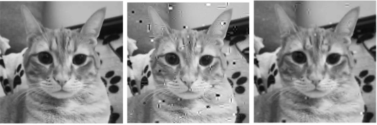
(a) PSNR=48.12, SSIM=0.99 (b) PSNR=36.20, SSIM=0.74 (c) PSNR=38.70, SSIM=0.94

Figure 11: (a): image after compression; (b): image after the Barcode Correction and Consensus; (c): image after post-processing.

Illumina machine. As can be seen in Figure 11, simply relying on Barcode Correction and Consensus is not completely sufficient in removing the sequencing noise from the image in Figure 11b, we must also perform post-processing to reduce the artifacting caused during the sequencing Figure 11c.

Because of this, we decided to add an additional form of error detection and correction as a post-processing step after the decoding of the synthesized DNA. This is not an entirely novel idea, in [58] the DNA decoding had been enhanced in a similar fashion by adding an inpainting step at the end of the process, with very convincing results. The main difference from our work will lay in the type of inpainting approach chosen, as our encoding and decoding workflows (and especially their reliance on the Discrete Wavelet Transform) dictate a somewhat peculiar approach to post-processing and de-noising.

A first necessity is the identification of the damage, that we will discuss in subsec-tion 2.6.1. This step, and its necessary automasubsec-tion, is a very difficult problem that both us and the authors of [58] had to find our way around. While the resulting solutions are very different, as each is tailored to the specifics of the work it is embedded in, this converging speaks of an underlying problematic that any work approaching post-processing in this way will need to prepare for.

After having identified where the damage is located, we need to try and correct it. We chose to use a sample based inpainting, a technique that relies on covering damage

using existing information from the rest of the image. The details of the chosen algorithm are presented in subsection 2.6.2. Other approaches are possible, and might work better with different types of encoding, but we performed extensive testing before choosing the method that in our opinion best suited our existing workflows.

2.6.1

Automatic Damage Detection

Automating the detection of erroneous pixels is a very complex process. Several methods have been proposed over the years, as the problem is central to a lot of image quality issues. Most of these act at a very low level in cameras and sensors [17],[27],[39] and are intended to detect either single or small clusters of erroneous pixels caused by a defect in the device itself. Other algorithms focus more on detecting noisiness; the algorithm from [21] can be used in this way, as can others [22]. Detection of the type of damage our reconstructed images exhibit would normally require a more complex approach, as the ones used in [37] and [36], to be viable.

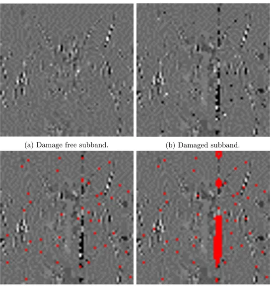
Luckily, our encoding process puts us into a relatively rare position. As our image was decomposed by the quantization process, each noisy subband carries less information than a full-sized image. Coupled with the way our advanced mapping works, this means that the visual distortion we incur in can be identified, in the subband, by a relatively simple algorithm partially inspired by the ones used in physical cameras [62]. While more advanced detection methods might have even more success, machine learning methods might again be investigated in future works if enough training data is available, the results we were obtaining with our own algorithm were deemed sufficient.

The damage detection process is composed of two separate steps. The first step is used to detect the damage caused by Substitutions during the sequencing. These only alter few pixels at a time, and generally result a type of damage resembling spots in the final image, that will be described in points 1 and 2 of section 3.1. Detecting these distortions is relatively straightforward since they only affect very small areas. As such, it is comparable to classical salt and pepper noise, which can be detected by simply checking the value of each pixel against that of its neighbors. The first step of the detection algorithm works in this same way, comparing the value of each pixel in the subband to

Algorithm 3: Damage detection. Input:

𝑆= (𝑆₁, 𝑆₂, . . . , 𝑆_𝑛) :damaged subband

𝑁 𝐸 𝐼 𝐺 𝐻 𝑆 = (N (𝑆₁),N (𝑆₂), . . . ,N (𝑆𝑛)) : neighborhoods of each value in 𝑆

𝑇 𝐻1 :step-1 threshold 𝑇 𝐻2 :step-2 threshold Output:

𝑀 :damaged values mask

𝑀 ←[ 0 ]; 𝐷𝐸𝑉 ←[ 0 ]; 𝑀𝐸 𝐴𝑁 ←[ 0 ] for 𝑖 ← 1 to #𝑆 do 𝐷 𝐸𝑉(𝑖) ← standard deviation(𝑁𝐸𝐼𝐺𝐻𝑆(𝑖)) 𝑀 𝐸 𝐴 𝑁(𝑖) ← mean(𝑁𝐸𝐼𝐺𝐻𝑆(𝑖)) 𝑀 𝐸 𝐴 𝑁_𝐷𝐸𝑉 ← mean(𝐷𝐸𝑉) for 𝑖 ← 1 to #𝑆 do if √ (𝑆(𝑖)−𝑀 𝐸 𝐴𝑁 (𝑖))2 𝐷 𝐸𝑉(𝑖) ≥ 𝑇 𝐻1 then

𝑀(𝑖) ← 1 // Indicate 𝑆 (𝑖) as potentially damaged.

if 𝐷 𝐸𝑉(𝑖)

𝑀 𝐸 𝐴 𝑁_𝐷𝐸𝑉 ≥ 𝑇 𝐻2 then