I
ALMA MATER STUDIORUM UNIVERSITA' DI BOLOGNA
SCUOLA DI SCIENZE
Corso di laurea in Analisi e Gestione dell’Ambiente
Assessment of the health impacts from air pollution
in Ravenna (Italy) using the EVA model
Tesi di laurea in “Processi di trasporto e dispersione degli inquinanti in
atmosfera” – CHIM/02
Relatore Presentata da
Prof. Alberto Modelli Marta Behjat
Correlatori
Prof. Massimo Andretta
Prof. Brandt Jørgen
Dr. Im Ulas
II
FOREWORD
Daily we hear about the economic and financial crisis, with such emphasis and concern to make it appear less important than the environmental crisis. In my opinion, if we are unable to contain the environmental crisis we cannot solve the economic crisis, because these two concepts, environment and economics, are related to each other. It is just this connection that pushed me to develop the topic of my final dissertation, paying specific attention to the health risk and related costs due to air pollutants.
III
ABSTRACT
The aim of this work is to assess the health impact from air pollution in Ravenna, a small Italian city located in the Pianura Padana. In this area the environmental pressure, because of air pollution, is worsened by unfavourable meteorological conditions. In fact Ravenna, in addition to being a large industrial area and one of the most important commercial harbours of Italy, has a temperate-continental climate characterised by a high relative humidity, because of the presence of fog, frequent thermal inversions during the winter and frequent conditions of wind lull. Because of these peculiar meteorological conditions and high pollutant emissions, e.g. from intense industrial activities, often alarming levels of air pollution occur, giving public health concern. These conditions stimulated the present study of the effects of air pollution on health in the area of Ravenna using the EVA model. This system was developed in the Atmospheric Modelling (ATMO) section of the Environmental Science Department of the Aarhus University (DK) to assess health-related economic externalities of air pollution, considering the main emission sectors and quantifying their relative importance in term of impacts on human health.
IV
SUMMARY
INTRODUCTION ... 1
AIM OF THIS RESEARCH ... 5
1. QUALITY OF THE AIR AND ITS MONITORING ... 7
2. LEGISLATION ... 9
2.1 Definitions... 11
3. AREA OF STUDY ... 12
3.1 Meteorological conditions ... 12
3.2 Emission Sources ... 15
3.3 Air Quality in Ravenna ... 16
4. MATERIALS & METHODS ... 18
4.1 Data Collection ... 19
4.1.1 Population Data ... 19
4.1.2 Emission Data ... 20
4.1.3 Authorization Integrated Environmental (AIE) ... 20
4.1.4 Geographic Information System (GIS) ... 21
4.1.5. Residential and commercial emissions ... 22
4.1.6 Industrial emission ... 22
4.1.6.1 Method for collecting data from AIE ... 22
4.1.7 Agricultural emissions ... 23
4.1.8 Vehicular emissions ... 24
4.1.9 Final emission data ... 25
4.1.10 Measurement data ... 27
4.2 Air Pollution Modelling ... 28
4.2.1 DEHM model ... 29
4.2.2 The UBM model ... 30
4.3 Validation of the models ... 31
4.3.1 Statistical evaluation ... 32
4.4 EVA model ... 35
4.4.1 Exposure-response functions and monetary values ... 36
4.4.2 Mortality ... 37
4.4.3 Morbidity ... 37
4.4.4 Valuation... 38
V 5. RESULTS ... 43 5.1 Scientific validation ... 43 5.2 Second validation ... 43 5.3 EVA results ... 46 5.3.1 Health impacts ... 46
5.3.2 The total health-related externalities ... 49
6. DISCUSSION AND OVERALL CONCLUSION ... 51
Attached A ... 55 Attached B ... 63 Attached C ... 71 Meteorological data ... 71 REFERENCES ... 72 ACKNOWLEDGES... 78
1
INTRODUCTION
The considerable increase of the industrial, commercial and agricultural development, and all human activities connected with the production of goods and services, have brought as a result different conditions of environmental pollution. But what is pollution? It is the establishment of “anomalous” conditions in an ecosystem, due to insertion of toxic substances, where people work and plants and animals have their life cycle. Therefore, pollution can modify the equilibrium between plants, animals (including humans) and climate of an ecosystem, especially by alteration of the air, water and soil.
Industrial emissions and incorrect disposal in the environment of non-biodegradable waste, waste water, plant protection products, fertilizers, hydrocarbons, dioxins, heavy metals and organic solvents can be considered as the main sources of pollution.
The chemical industry produces, each year, thousands of compounds, but we have scarce scientific information about their toxicity and real impact on health and environment.
Therefore, on the one hand the economic growth delivers better living conditions to millions of people around the world through industrial development, improved transport, modern energy systems and other technological facilities, while, on the other hand, it often causes serious problems associated with pollution. In particular, the attention of the present study is specifically turned to air pollution.
Since the late 1970s, air pollution has been one of the main environmental policy concerns of the European Union. According to the European Environment Agency (EEA), air pollution is “the presence of contaminant or pollutant substances in the air at concentrations that interfere with human health or welfare, or produce other harmful environmental effects”.
2
Air pollution constitutes a severe problem for the environment and, consequently, for the human health. In Europe there are excessively high concentrations of air pollutants leading to health and economic issues associated to these pollutants. A large portion of the European population lives in areas where the emission limits [1], as defined by Directive 2008/50/CE, are exceeded.
The Directive 2008/50/CE [2] of the European Parliament and Council (21th May 2008) deals with the quality of the air, and is aimed to obtain a cleaner air in Europe. This directive establishes targets to be reached within 2020 to improve the quality of the air, the human health and the quality of the environment. Moreover, the same Directive indicates how to evaluate and reach these objectives, and implements actions in the case the fixed rules are not followed. In addition, it provides public information.
The main effect of emissions of gaseous pollutants (e.g., carbon monoxide, sulphur dioxide, nitrogen oxides, benzene, and particulate matter) in the atmosphere is a chemical and physical alteration of the air.
According to the European Commission [3], every year more than 400.000 people in the UE die prematurely as a consequence of air pollution. Another 6.5 million people fall sick because air pollution causes diseases such as strokes, asthma and bronchitis. Air pollution also harms our natural environment, impacting both vegetation and wildlife: almost two thirds of the European ecosystems are threatened by the effects of the air pollution.
Air pollution, as a side-effect to economic growth and development, is currently threatening citizens’ health, thus leading to high expenses and severe environmental damages all around the world.
In fact, the presence of pollutants in the atmosphere results in a large damage to public health and economics of a country. These two factors, economy and health as evaluated by analysis of Environmental Impact Assessment (EIA), constitute the topic of my final dissertation.
3
According to current estimates, the joint effects of ambient and household air pollution cause 7 million premature deaths globally each year, representing one eighth of the total deaths worldwide [4]. From the economics point of view, there is evidence that air pollution imposes remarkable costs to society, of the order of magnitude of several trillion dollars per year, globally. Economic analyses show that, considering the impact of air pollution on both health and economics, the benefits of a cleaner air would be extremely large.
In Italy the economic costs caused by the effects of air pollution on health are evaluated to be 4.7% of GDP (Gross Domestic Product), while in ten countries of Europe the cost is slightly higher than 20% of the GDP [5].
According to the World Health Organization (WHO)1 more than 90% of
European citizens are exposed to annual amounts of air pollutants which exceed the limit established by the WHO guidelines (Economic cost of the health impact of air pollution in Europe - WHO 2015).
In 2012, 482000 premature deaths have been ascribed to the outdoor air quality, and 117200 premature deaths to the indoor air quality [6].
Therefore illness and premature death caused by air pollution not only are a damage for public health, but also for economics, costing to Europe about 1463 billion euro a year. According to the WHO, this cost is associated with about 600 thousand premature deaths caused by air pollutant.
The purpose of this work is to evaluate the effects of air pollution on the economy and human health. The area of study is the city of Ravenna, situated in the Emilia Romagna Region (NE Italy) on the Adriatic Sea.
The city of Ravenna includes a large industrial area and one of the most important commercial harbours of Italy. Despite the air quality in the Province of
1WHO is directing and coordinating authority on international health within the United Nations’ system.
WHO works together with policy-makers, global health partners, civil society, academia and the private sector to support countries to develop, implement and monitor solid national health plans.
4
Ravenna has significantly improved over the last decades, and concentrations of some pollutants, such as particulate matter, nitrogen oxides, and ground-level ozone, are now levelling off, air pollution monitoring and related health problems, particularly in the urban areas, remain an important issue. Road transport, harbour and industrial activities and burning of fossil fuels are the main sources of these pollutants.
A reliable assessment of the health-related costs connected with air pollution is a powerful tool for decision making, since these costs must be taken into account as well as other social costs.
In order to make an assessment of the influence of external cost of the health impact because of air pollution on the society, an integrated model system has been employed.
The development and the implementation of models allow to simulate the effects of air pollution, paying specific attention to the negative consequences on public health and economy.
For this kind of study, we used an atmospheric health impact assessment model (EVA: Economic Valuation of Air Pollution) that has been developed in the ATMO (Atmospheric Modelling) section of the Environmental Science Department of the Aarhus University.
The EVA system has been applied to the Ravenna city to assess health-related economic externalities of air pollution considering the major emission sectors and quantifying their relative importance in term of impacts on human health and related external costs in the area.
5
AIM OF THIS RESEARCH
This thesis addresses the economic cost of public health impacts of air pollution in Ravenna, Italy. The idea of this project arise from the need to inform the community about the health risks caused by air pollution and their costs on the society, in order to push people to face this problem.
In the Province of Ravenna the most frequent meteorological condition, in all seasons, is a “meteorological stability” associated with the lack of thermodynamic turbulences and small variations of the wind speed with altitude.
The pollutants emitted from human activities influence directly the quality of the air that we breathe, being thus responsible for the impacts on the health and environment. Many of these pollutants are considered potentially dangerous for the health and corrosive for the cultural heritage. The health impacts of air pollution carry many significant financial and economic implications, not only in terms of social costs and mortality, but also household, hospital and public budgets and, therefore, imply decision making within and outside the health sector.
The quality of the air is a typical indicator of the impact of human activities on the quality of life, and accordingly on economy. Different kinds of instruments, through regulations and monitoring, have been developed to face and assess this problem.
The present work describes a methodology to evaluate the economic cost of health impacts using the EVA model. The EVA system, based on the impact-pathway chain, allows to assess the health-related economic externalities of air pollution resulting from specific emission sources and to support policy-making with respect to emission control [7]. In fact the main goal of this work is to identify the anthropogenic emission sources in Ravenna that contribute the most important impacts on human health.
6
In this study, we apply the EVA model to Ravenna to examine the contributions from four sectors, or SNAP (Selected Nomenclature for Sources of Air Pollution) emission sectors, and to quantify their relative importance in terms of impacts on human health and related external costs.
The EVA model is based on an Eulerian atmospheric model for regional transport and chemical transformation of air pollutants (Danish Eulerian Hemispheric Model - DEHM) and an urban background model (UBM).
The purpose of this work is to evaluate the health impact and the external costs of air pollution using the EVA model integrated with estimates of exposure from the DEHM (Danish Eulerian Hemispheric Model) and UBM (Urban Background Model) models. The exposure-response functions (ERF) used in EVA are based on the assessment of European experts in public health and consultation with the WHO [8].
This work was carried out in the ATMO section of the Department of Environmental Science of the Aarhus University with the collaboration of the Department of Analysis and Management of Environment of the University of Bologna.
7
1. QUALITY OF THE AIR AND ITS MONITORING
The air pollution is defined by the Legislative Decree 152/2006 as “each change of the atmosphere because of the introduction of one or more substances whose properties can create a risk for the human health or for the quality of the environment or damage material goods or compromise the legitimate uses of the environment”. Most of the substances that are emitted in atmosphere can change and became dangerous for the health and for the environment. These kind of species are evaluated and analyzed on the basis of their effects, temporary or irreversible, immediate or long-term effects. So these species are classified on the basis of the limit of concentration at which they become dangerous [9].
Air pollution is the result of emissions from various sources with extremely different features regarding height and temporal variability. The most important pollutants are the so-called primary pollutants, which originate from fossil fuels in various ways, such as CO2 (from combustion), impurities or additives (typically
sulphur in oil and lead in petrol), CO, NOx and hydrocarbons. Some pollution comes
from industrial activities. Typical agricultural emissions are NH3, CH4 and NOx. These
pollutants are also naturally emitted, but human activities have increased the emission manifold. Compounds formed in the atmosphere through reactions of primary pollutants are referred to as secondary pollutants [10].
The regulations about air pollution and its effects on the human health and environment consider two important aspects:
Evaluation of the level of pollutions in the air (by means of measurements, calculus and esteem)
Management of the quality of air through actions suitable for programming and planning its protection, rehabilitation and improvement of the quality [11].
8
On the basis of the Legislative Decree 155/2010, the valuation of the quality of air depends on a network of measurements of the pollutants and on the system of valuation [9]. To evaluate the concentrations of air pollutants a monitoring network is used, which supplies hourly measurement. This network consists in a series of fixed stations located on the entire national territory [12]. The data collected are elaborated and analyzed by the Regional Agency responsible for each area. For instance, in Italy these Agencies are designated as ARPA (Regional Agency for the Protection of the Environment). The data are then collected in a database that can be national (e.g., Brace2) or European (e.g., AirBase3). The locations of the
stations, the choice of the analyzers installed in each station, the sampling techniques used and the analysis of the results are established by national and regional regulations, which take into consideration the following pollutants:
- Gas: compounds that contain sulphur, nitrogen, carbon and ozone. - Particulate (PM10 and PM2.5) [9].
2 http://brace.sinanet.apat.it/
9
2. LEGISLATION
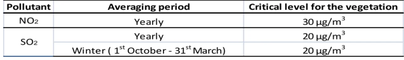
In Italy the first procedural guidelines about the air were given by the framework law 651/66, followed by other regulatory national and local rules. The aim of the regulation was to “reach a level of the quality of the air that doesn’t bring negative consequences or risks for the human health and for the environment”. This legislation was adopted to reduce the exposure to air pollutants, by decreasing emissions and fixing limits to the concentrations of pollutants. Today, the Community measures are managed by the Directive 2008/50/EC (European Legislation), while the Italian measures are managed by the Legislative Decree of the 13 August 2010, n. 155 [9]. This Decree, subsequently amended and supplemented in 2012 (Legislative Decree 250/2012), gives information about zoning, and also on limit and target values and critical levels [11].
Table 1. Limit values (Annex XI D.Lgs 155/2010)
Pollutant Averaging period Critical level for the vegetation
NO2 Yearly 30 μg/m3
Yearly 20 μg/m3
Winter ( 1st October - 31st March) 20 μg/m3 SO2
Table 2. Critical levels for the vegetation (Annex XI D. Lgs 155/2012)
Pollutant Averaging period Limit value
Hourly (not to be exceeded more than 24 times per year) 350 μg/m3 Daily (not to be exceeded more than 3 times per year) 125 μg/m3 Hourly (not to be exceeded more than 18 times per year) 200 μg/m3
Yearly 40 μg/m3
CO Max daily average in 8 hours 10 μg/m3
Daily (not to be exceeded more than 35 times per year) 50 μg/m3
Yearly 40 μg/m3
PM2.5 Yearly 25 μg/m3
NO2 SO2
10
Purpose Averaging period Target value Deadline
Protection of the human health
Max daily average in 8 hours per year
120 μg/m3 to not exceed over 25 days per year as a
average on 3 years 2013 Protection of the vegetation AOT40 calculated on the base of hourly values from
May to July
1800 μg/m3 h as a
average on 5 years 2015
Protection of the human health
Max daily average
in 8 hours per year 120 μg/m3 No defined Protection of the
vegetation
AOT40 calculated on the base of hourly values from
May to July
6000 μg/m3 No defined
Long-term targets
Table 3. Target values and Long-term target for the Ozone (Annex VII D.Lgs. 155/2010) [13]
At the European level, the Council and the European Parliament reached an agreement on June 30th 2016, to reduce the emissions of pollutants in the
atmosphere. This new Decree establishes limits more stringent than the previous ones, to be adopted from 2020 to 2029, and even more restrictive from 2030 on. The Decree aims to address the risks for the human health and for environment, but also to extend the European legislation at the national levels (following the revision of the Göteborg Protocol4 in 2012 ). The new Decree establishes the national limits
for five pollutants: NO2, SOx, NMVOC (Non Methane Volatile Organic Compounds),
NH3 and PM. The limits that each nation should respect in the years 2020-2029 are
those established by the Göteborg Protocol, but from 2030 on the limits will become more severe. According to various estimates, these new limits will reduce the effects of air pollution on human health by 50%, compared to 2005 [15].
The region Emilia-Romagna has developed its own legal regime, in line with the national legal regime. In particular, the region has entrusted the monitoring of
4 The Göteborg Protocol (1999) is relative to the abate acidification, eutrophication and atmospheric ozone
11
air pollution to ARPA and implemented the Legislative Decree 155/2010 at a regional level through the D.G.R.5 n°2001, dated 27/12/2011 [11].
2.1 Definitions
Limit Value: is the value established on the basis of scientific knowledge in order to avoid, prevent and reduce negative effects on the human health and the environment, that have to be achieved within the scheduled deadline; after the deadline this values have not to be exceeded.
Critical Value: is the value established on the basis of scientific knowledge over which negative effects on “receptors” like trees, plants or natural ecosystem, except for humans, may appear.
Target Value: is the value established in order to avoid, prevent and reduce negative effects on the human health and the environment, to be achieved, when possible, within a deadline [13].
12
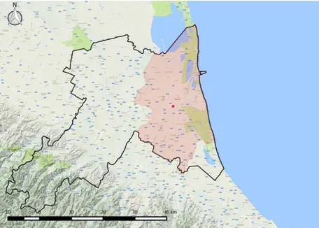
3. AREA OF STUDY
The area considered in this study is Ravenna, in Emilia-Romagna, north-east of Italy, a small Italian city on the Adriatic sea with approximately 153900 residents in 2012 (652.9 km2 and 4 m above sea level).
3.1 Meteorological conditions
Ravenna is located in the Pianura Padana, where the environmental pressure associated with air pollution is worsened by unfavourable meteorological conditions. In fact, Ravenna is characterized by a continental-temperate climate with high relative humidity, because of the fog, frequent thermal inversion conditions during the winter and frequent wind lulls. Information about temperature, precipitations, wind speed and direction is recorded by several meteorological stations located in the Province of Ravenna, one of them being located in the urban area (Figure 1).
Temperature: Figure 2 reports the average, minimum and maximum monthly temperatures for the year 2014, as measured by the meteorological station of ARPA in Ravenna.
Figure 1. Meteorological station in Ravenna
13
Figure 2. Average, minimal and max monthly temperatures for the year 2014 [16]
Precipitation: the total monthly precipitations and the number of days where the precipitations exceeded 0.3 mm are shown in Figure 3. In this case two meteorological stations are involved in the measurements: one in the heart of downtown, the other in the harbour area (Porto San Vitale). The value of 0.3 mm was chosen as a threshold of the total daily precipitations because below this value the critical conditions for accumulation of the PM10
are favoured, in agreement with the SIMC (Service Hydro Weather Climate). In fact the SIMC states that precipitations lower than 0.3 mm and index of ventilation lower than 800 m2/s facilitate a concentration increase of PM
10 in
atmosphere. The precipitations measured in the harbour area were lower than those of the urban area.
Figure 3. Total monthly precipitations and number of days with daily precipitations over 0.3 mm for the year 2014 [16]
14
Wind Speed & Wind Direction: Figure 4 shows the wind rose, as recorded by the urban meteorological station, which describes the wind trends. The distribution of the speeds shows that values lower than 3 m/s is prevailing over a whole year. The most frequent wind directions are W-NW and NW, to a lesser extent E-SE.
Figure 5 displays the prevailing season wind directions and speeds. In winter and autumn wind directions do not look like dispersive. In summer small variations are observed because of the influence of sea breezes with direction E-SE. Spring is the season in which the highest variability is observed.
So because of these meteorological condition and the intensive industrial activities, in Ravenna there is an alarming air pollution and the relative public health concern [16].
15
Figure 5. Seasonal wind rose for the meteorological station of Ravenna [16]
3.2 Emission Sources
Ravenna is characterized by the presence of emission sources which cause a significant environmental pressure. The emissions of pollutants in atmosphere are the result of intense industrial activities. In fact, in addition to a strong agricultural activity in its surroundings, Ravenna has a large industrial area and an harbour among the most important in Italy. The industrial and dock areas are characterized by the presence of chemical and petrochemical plants, two thermal power stations, metallurgical companies, construction factories and port activities. The harbour, one
16
of the most important in the Adriatic Sea, is of great support to the economy of Ravenna. However, this economic development is causing serious problems for the environment. In fact in 2000 a protocol of understanding was signed by 16 companies to achieve the ISO140016 and EMAS7 certifications [17].
3.3 Air Quality in Ravenna
The ARPA of Ravenna reports in the web the results of the monitoring of the quality of the air for each pollutant [27].
Sulphur dioxide (SO2)
The concentrations in 2015, as well as in the last years, are low and well below the limit value. Therefore, it is not a problem to exceed the limit value for SO2. Moreover, the concentration profile shows that there is a trend
towards a further improvement. Nitrogen dioxide (NO2)
The limit value of the annual average of NO2 is not exceeded since 2010, its
concentration being decreasing since 2007. A slight increase observed in 2015 (relative to 2014) was ascribed to the occurrence of unusual meteorological conditions. The highest concentrations are measured in the urban area (Zalamella station), due to vehicular traffic.
Carbon monoxide (CO)
The values of CO concentration are decreasing, especially since 2007. The limit value, to protect the human health, established by the D.Lgs. 155/20101, was never exceeded. Actually, the measured values are much lower than the limit value, and display a decreasing trend over the last years.
6 The acronym ISO1401 identifies an environmental management standard (EMS) that establish the
requirements for a management of environment for each organization.
7 EMAS (Eco-Management and Audit Scheme) is a voluntary instrument created by the European
Community to which the organizations can adhere to evaluate and improve their environmental performances.
17
Ozone (O3)
The values of O3 concentration in 2015 are very critical, exceeding both the
limit and target values (240 μg/m3 and 120 μg/m3 8). There is a strong
correlation between O3 concentrations and meteorological conditions. In fact
the warm summer of 2015 favored the increase of O3 levels compared to 2014. The observed trend shows that there is a nearly constant concentration of O3 in whole the region [16].
18
4. MATERIALS & METHODS
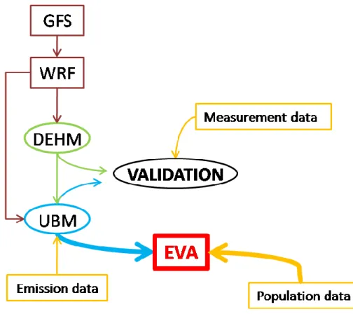
In this work a detailed analysis of health-related external costs associated with the major emission sectors and their relative contributions is performed using the EVA model. The application of this model requires the use of other two models: DEHM and UBM. In turn, to adopt these models it is necessary to collect all the data relative to the emissions of the area of Ravenna. Four kinds of emissions sectors are considered for this case of study: residential/commercial, industrial, agricultural and vehicular. In addition to the emission data, it is necessary to collect data regarding the population distributed in a grid, the concentration measurements and meteorological data (Attached C) . The scheme of Figure 6 represents the way these data are used.
Figure 6. The scheme displays how the meteorological data, from the GFS (Global Forecast System), WRF (World Research Forecast) and meteorological stations, emission measurements and population data are used with the DEHM, UBM and the EVA system.
19
4.1 Data Collection 4.1.1 Population Data
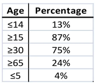
A gridded data set was obtained from the GEOSTAT 2011 grid dataset [18] covering all Italy. The grid is formed by cells 1km x 1km wide. For each cell the number of people that are present is indicated, thus allowing evaluating the distribution of the population. We have also calculated the percent contributions from various ages applying a proportion. It is important to analyse the health outcomes as a function of age as different age groups respond differently to pollution. We have subdivided the population into five groups of age, and the equation used is provided in Eq. 1.
Eq. 1 Age Percentage ≤14 13% ≥15 87% ≥30 75% ≥65 24% ≤5 4%
Table 4. percentage of the age of the population of Ravenna
where Pop (Age)(1) andTot Pop(1) are taken from the website ISTAT [19]. These data
refer to the year 2011. The total population of Ravenna is 153740 inhabitants, while
Tot pop (2) is the population of the grid dataset (163763). Eq.1 is used to calculate the
20
Figure 7. Population distribution of Ravenna for each cell (1km x 1km)
4.1.2 Emission Data
To use the EVA model is necessary to collect emission data for each cell (1 km2
resolutions), for residential/commercial, agricultural and vehicular emissions, and from each factory stack for industrial emissions. All data gathered lead to an emission expressed in kg/year. For each chimney and each cell we have determined the coordinates. The pollutants considered are: NOx, SOx, NMVOC, CO, TSP, PM10,
PM2.5. During the data collection step, I used two instruments: the AIE
(Authorization Integrated Environmental) and the Q-Gis (Quantum Geographic Informatics System).
4.1.3 Authorization Integrated Environmental (AIE)
To evaluate the emissions from all industries in the area of Ravenna I decided to consult the AIE of each industry. This document authorizes the activities of an industry. These activities have to guarantee compliance with the requirements specified in the second part of the Legislative Decree 152/2006. This Decree is
21
relative to industrial emissions (prevention and integrated reduction of pollution). This Authorization is released to the industries listed in the VIII attachment of the second part of the same Decree [21].
Each authorization reports complete information about the factory: hours and days of activity, position, productive processes and emissions in water, soil and air. In the chapter dedicated to the air, the stack characteristics are described: height, coordinates, hours of activity, payload and kinds of emitted pollutants.
In AIE the emissions are classified as funnelled and fugitive emissions. In the fifth part of the Legislative Decree 152/2006 [22] the two kinds of emissions are defined. Funnelled emissions involve the discharge of pollutants from a release point, for example from a stack. Before their release in atmosphere, funnelled emission can be treated to reduce, or delete, the pollutants. Essentially, the treatment systems can be of two kinds: one to remove the pollution, the other to capture it. The latter allows the recovery and reuse the pollutants, otherwise the pollutants can be processed and conferred like waste. In contrast, fugitive emissions can not be located in specific points, they are considered as area sources.
4.1.4 Geographic Information System (GIS)
The GIS system is able to assemble, memorize, modify and visualize geographic information, that is, data identified on the basis of their geographical locations. This instrument was used:
- to collect all geographic information used in the area of study - for processing and analyzing the collected data
- for managing the input file according to the mathematical model of dispersion of pollutants
22
- for the management of the collected and elaborated data during the research in a geo-database
4.1.5. Residential and commercial emissions
The term “residential/commercial” is used to indicate emissions from combustion in commercial, residential and institutional activities, where combustion is used for domestic heating, water heating and food preparation. The data of Table 5 were derived from the total provincial emissions reported by ARPA in the inventory of emissions in atmosphere for the year 2010 [20].
Macro sector Sector CO SO2 COV CH4 NOx PTS CO2 N2O NH3 PM10
No industrial combustion Residential plant 6595 280 2473 436 787 489 929 96 12 467 Table 5. Pollutants (Mg, Gg for CO) emitted per year from no-industrial activities in the whole Province of Ravenna.
Knowing the total emissions, the total population, the population for each cell of the province of Ravenna, it is possible to calculate, via a mathematical proportion, the emission associated with each cell. For example, in the case of CO:
Eq.2
The total provincial population (393623) and the population of each single cell are given by the grid dataset (2011) [18].
4.1.6 Industrial emission
4.1.6.1 Method for collecting data from AIE
The required authorizations are of two kinds: one is released from the Province, the other from the State. In the State authorization, the manager declares
23
the quantity of pollutants emitted from each chimney. From these declarations I could obtain data relative to the pollution emitted from the four different sources. In the authorization released by the Province, the quantity of pollutants emitted is not declared. However, from the information about the characteristics of the stacks, it was possible to estimate the emissions applying the following formula:
Eq. 3
where Nm3 is the volume normalised to P=1 atm and T= 0 °C.
The application of this formula allows to calculate the flow of thepollutants emitted from the stacks.
As far as the fugitive emissions are concerned, we decided to distribute them in each grid cell of the domain. The industrial fugitive emissions, as taken from IEA, were located in the same area where the industry that emitted them is placed.
4.1.7 Agricultural emissions
Over the industrial, residential and commercial emissions, the agricultural sector is one of the biggest source of GHG emissions. The fundamental GHG emission is the enteric fermentation (methane that is released from the livestock during the digestion). Another kind of agricultural emissions are caused by the use of synthetic fertilizer [60]. To evaluate the agricultural emissions, the same method adopted for industrial emissions was used. Before collecting the data, I had to classify the IEA as authorization for agricultural activities, for example, pig farming or poultry farming.
24
4.1.8 Vehicular emissions
To collect the data regarding the vehicular emissions, it was decided to consider the total provincial emission, percentage of emission for each kind of street and, finally, the length of the streets (the total streets and the streets in each cell). The data relative to the Province, expressed in ton/year (kton/year for CO), are inserted in the inventory of emissions in atmosphere for the year 2010 [23], the percentage of emission for each kind of street is inserted in the PhD thesis of S. Marinello [9]. The length of each street was obtained with Q-Gis (Quantum Geographic Information System).
The percentages of emission are the results obtained from an unbundling model of emissions from vehicular traffic. The data used were provided by ARPA, as obtained from traffic data measured in conformity of the representative road section; thus it is possible to have an estimate of vehicular traffic in the urban area of Ravenna. These percentages allow one to assign to each kind of street the total provincial emission given by the inventory [9].
Province CO SO2 NMCOV CH4 NOx PTS CO2 N2O NH3 PM10
Ravenna 5928 32 1116 101 5387 510 1103 31 69 413
Table 6. Pollutants (Mg, Gg for CO) emitted per year from vehicular in the whole Province of Ravenna
Kind of street PM10% NOx% CO% SO2%
Urban street D 0.25 0.24 0.28 0.26
Urban street E 0.17 0.16 0.19 0.17
Local road F 0.42 0.43 0.35 0.40
Other 0.16 0.17 0.18 0.17
Table 7. Percentages of emissions for each kind of street in Ravenna
The road network downloaded from Open Street Map (OSM) has been superimposed on the grid in Q-GIS. Q-GIS allows to measure the length of the
25
streets in each cell, as well as the total length. Therefore, knowing the total Provincial emission for each pollutant, the total length of the streets and their length in each cell it is possible to determine the vehicular emission for each cell, applying the following proportion:
Eq. 4
where Tot stands for total and Len for length.
For the present case of study four kind of streets were considered: - Urban street D: independent roadway or road separated by traffic divider; in OSM is highway = tertiary
- Urban street E: a single-carriage way with at least two lanes; in OSM are highway = residential and living street
- Local road F: urban or suburban road not considered in other types of roads
- Other: street whose classification is not defined; it is used as temporary tag for a street whose classification is unknown; in OSM are highway = motorway, primary, secondary and track [24].
4.1.9 Final emission data
In the present case NOx, SOx, NMVOC, CO,TSP, PM10 and PM2,5 have to be
considered to run the UBM model. These data are collected in two files: one for pollutants emitted from stacks, the other for pollutants associated with each cell. Unfortunately, the Italian Authorizations do not consider the particulate (PM10 and
26
PM2.5) but just the total suspended dust (TSD). An evaluation of PM10 and PM2.5 from
TSD was obtained by consulting the emission factors provided by the EMEP/EEA Guidebook [25]. As far as the emissions for each cell are concerned, we have data only for PM10, not for PM2.5. It was possible to esteem PM2.5 from PM10 on the basis
of the emission database from EMEP/CEIP [26]. The different kinds of emission are classified according to the SNAPS:
- SNAP 01: no industrial emission - SNAP 02: Vehicular emission - SNAP 0201: Urban Street D - SNAP 0202: Urban Street E - SNAP 0203: Local Road F - SNAP 0204: Other
- SNAP 03: Agricultural emission - SNAP 04: Industrial emission
27
Fig. 8c Fig.8d
Figure 8 (a,b,c,d,e). Distribution of the emissions for various pollutants.
Fig. 8e
4.1.10 Measurement data
The observed air pollutant concentrations from different monitoring stations were obtained from the ARPA network. These stations continuously measure hourly concentrations. In all environments (urban, rural or industrial) various pollutants, like CO, SO2, O3, PM2.5, NO2, C6H6 and PM10, are monitored.
28
In this work, three stations have been considered for the area of Ravenna, one located in the urban area and two in rural areas.
The measured concentrations and information about each station of the Ravenna area (Table 8) were taken from the ARPA website of Emilia Romagna [27].
Stations Elevation (m) Kind of Area Longitude Latitude
Caorle 4 Urban zone, characteristic residential zone 12,22539 44,4193 Delta Cervia 0 Suburban zone, characteristic agricultural zone 12,33225 44,2839 Ballirana 6 Rural zone, characteristic natual zone 11,98236 44,5274
Table 8. Characteristics of the four stations
4.2 Air Pollution Modelling
The use of air pollution models is useful to supplement and extend the information obtained from various measurements, as a tool for the interpretation of the measurements. In general, air quality models may be used for a variety of different purposes in environmental monitoring, management and assessment, such as in the characterisation of air pollution. Another important use of these models is the prediction of pollution loads and levels in the future. Models are the only option for providing short term predictions of air pollution at a regional and local scale. Air pollution is a trans-boundary problem, but the development of integrated modelling frameworks allows to describe atmospheric long-range transport of pollutants and all the processes that take place during their transport. Some of these models simulate the fate of individual air parcels along trajectories (referred to as Lagrangian models), while other models describe the concentration and processes in a fixed grid (Eulerian models). Eulerian models are able to describe the dispersion of the pollutants on a large scale, covering a large domain, giving results on a grid [10].
29
Eulerian models can calculate the variation of concentration (ρ) as a function of time (t) in a fixed point (partial derivate, ∂ρ/∂t) [30]. Lagrangian models are suitable to describe the dispersion in proximity of the source, handling sharp gradients and giving good results when used on a short scale [10]). Lagrangian models calculate the variation of concentration (ρ) as a function of time (t) in a parcel that moves in the space with a given speed (substantial derivate, dρ/dt) [30].
4.2.1 DEHM model
The Danish Eulerian Hemispheric Model (DEHM) is a three-dimensional, offline, large-scale, Eulerian, atmospheric chemistry-transport model which aims to study long-range transport of air pollution in the Northern Hemisphere and Europe. The model was originally developed in the early 1990’s to study the atmospheric transport of sulphur and sulphates into the Arctic region, but it has been continuously modified, and now it can be applied to the dispersion of 58 chemical compounds, 8 class of particulate matter and 122 chemical reactions [31].
An important development of the model consists in the ability to obtain a high resolution over limited areas, joining the DEHM to several emission databases and accounting for different conditions, such as wet and dry deposition [32, 33, 34, 35].
The model setup used in this study includes three two-way nested domains. The first domain covers most of the Northern Hemisphere, the second domain covers Europe and the third domain covers North Europe. Each domain has a different resolution, the first domain with a resolution of 150 kmx150km, the European domain with a resolution of 50kmx50km and the third domain with a resolution of 16.67kmx16.67km [31]. The model configurations used in the present work are the first and the second domain. The necessary information to run the DEHM model concerns input data of meteorology and emission, applying the following equation:
30 Eq.5
where c is the mixing ration, t is time, u, v, and
are the wind-speed components in the x,y (horizontal) and (vertical) direction, respectively. Kx, Ky and Kσ are
dispersion coefficients, while P and L are production and loss terms, respectively [31]. The meteorological data used in the DEHM model come from the WRF model (Weather Research Forecasting) that, in turn, uses data coming from the GFS (Global Weather Forecast System). The WRF is an open source software which collects meteorological data and represents them on graphic maps that give information about the evolution of atmospheric conditions in the time [36]. This model is based on the data supplied from the global system GFS that provide atmospheric and land-soil variables, such as temperature, wind speed, precipitation, land-soil moisture and atmospheric ozone concentration [37]. The output of the DEHM model is used for the validation, but also to run the UBM model.
4.2.2 The UBM model
The Urban Background Model (UBM) calculates the urban air pollution on the basis of emission inventories, with a spatial resolution of 1kmx1km. The UBM is a Gaussian plume model that allows to calculate the dispersion and transport of air pollutants to every receptor point, accounting for the photochemical reactions of NOx and O3. This model is constantly developed, and provides a realistic spatial
distribution of the pollutant concentrations over the grid, also around large point sources. The vertical dispersion is assumed to be linear (from the initial vertical dispersion and up to the mixing height) with the distance to the receptor point. Horizontal dispersion is accounted for by averaging the calculated concentrations over a certain, wind-speed dependent, wind direction sector, centered on the
31
average wind direction using a Gaussian distribution [38]. The meteorological data, used to have information about the distribution of pollutants in the space, derive from the WRF. In the UBM model, in addiction to consider the meteorological data, it is necessary to use the regional air pollution forecast from the DEHM, which gives information about the distribution of pollutants in areas around the area of study, and emission data. The model calculates the concentrations of NOx, NO2, O3, CO,
PM10 and PM2.5 in each point, which in the case of my work are the measurement
stations, and over all the grid. The first results, relative to the measurement stations, were used to validate the model. The species considered are NO2, O3, CO, PM10 and
PM2.5, because the data that I collected from the database of the measurements
include only these species in the three-year period (2010, 2011, 2012) considered in this study. The next results were used as input data for the EVA model.
4.3 Validation of the models
At the end of this first stage of the work, we get the results from the DEHM and UBM models, measurements and meteorological data (observations), i.e., all the information necessary to start the validation. The validation includes comparing simulated air pollutant levels from the UBM and DEHM model with the observed levels using statistical parameters. The purpose of the validation is to evaluate how the model is performing against a set of observation. The model validation is performed comparing model results with observation using some statistical measures. In this way we can see if the results that we get from UBM and DEHM model are congruent with the data relative to observations. The discovery of an error during the validation is for sure a benefit for the quality of the models results and it requires an improvement in the different modelling compartments such us emission, meteorology or chemistry.
32
4.3.1 Statistical evaluation
Statistical evaluation was performed using the “openair” package of the R software, which aims to provide a collection of open-source tools for analysis of air pollution data. This statistical/data analysis software allows to compare the results supplied by a model either with measurements or with other models. The factors considered for the statistical evaluation are indicated in the equation reported below, where Oi represents the ith observed value and Mi represents the ith modelled value for a total of n observations.
FAC2 (Fraction of prediction within a factor or two)
The fraction of modelled values within a factor of two relative to the observed values is the fraction of the model predictions that satisfy :
Eq.6
MB (Mean Bias)
The mean bias provides a good indication of the mean over- or
underestimation of the predictions. The mean bias has the same units as the quantities being considered.
33
MGE(Mean Gross Error)
The mean gross error gives a good indication of the mean error regardless of whether it is an over or under estimate. The units of the mean gross error are the same used for the quantities being considered.
Eq. 8
NMB (Normalized mean bias)
The normalized mean bias is useful for comparing pollutants that cover different concentration scales, the mean bias being normalized by diving MGE? o MB? by the summation of the observed concentrations.
Eq. 9
NMGE (Normalized mean gross error)
The normalized mean gross error further ignores whether a prediction is an over or under estimate.
34
RMSE (Root mean squared error)
The RMSE, commonly used in statistics, provides a good overall measure of the proximity of the modelled values to the measured ones.
Eq. 11
r (Correlation coefficient)
The correlation coefficient is a measure of the strength of the linear relationship between two variables. The correlation coefficient r is +1 (or -1) in the case of a perfect linear relationship, with positive or negative slope, between two variables, while a correlations coefficient r = 0 indicates the absence of a linear relationship between the variables.
Eq. 12
where M and O are the standard deviations of the M and O sets of data,
respectively.
COE ( Coefficient of Efficiency)
The COE is used to interpret the measuring model performance. A perfect model has a COE=1. For the negative values of COE, the model is less effective than the observed mean in predicting the variation in the observations. A
35
COE=0 implies that the model is not able to predict the observed values better than the observed mean.
Eq. 12
IOA (Index of Agreement)
The IOA is commonly used in model evaluation. It ranges between -1 and +1, values approaching +1 representing better model performances.
Eq. 13 [13]
4.4 EVA model
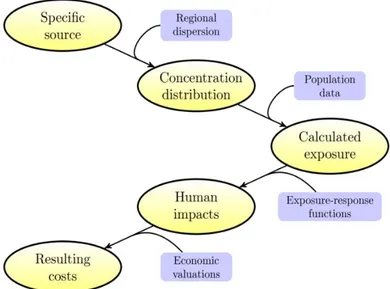
The concept of the EVA system [39, 40, 41, 42, 43, 44, 45] is based on the impact-pathway chain [46, 47]. The EVA system consists in a regional-scale chemistry transport model, which include gridded population data, exposure-response functions for health impact and economic valuations of the impact from air pollution. The system was originally developed to evaluate site-specific health costs related to air pollution, such as those deriving from specific power plants [41].
36 Figure 9. A schematic diagram of the impact-pathway methodology
Figure 9 reports a schematic diagram which describes the methodology of the EVA model. Starting from site-specific emission results, through a regional dispersion described in this study with the DEHM and UBM models, a concentration distribution is obtained. This concentrations, together with detailed population data, can be used to estimate the population-level exposure. Using exposure-response functions and economic valuations, the exposure can be transformed into impacts on human health and related external costs [8].
4.4.1 Exposure-response functions and monetary values
To calculate the impacts of emissions from a specific source, i.e., the response to the exposure to pollution, an exposure-response function (ERF) is used. The follow formula (Eq. 14) combines concentration (δc) and population data to estimate human exposure, and then the response (R):
37
where α is an empirically determined constant for the particular health outcome typically obtained from the published cohort studies, P the affected share of the population [8]. This function is an approximation based on cohort studies of 500000 individuals [48] also supported by the joint World Health Organization/UNCE Task Force on Health [49, 50]. All the exposure-response functions (shown in Tab. 9 ) are applicable to the European conditions. The chemical compounds related to human health impacts included in the EVA model are O3, CO, SO2, SO42-, NO3- and PM2.5.
Furthermore, NH4+ is included when it contributes to the particle mass through
reactions with sulphates or nitrates [8]. In the case of the present study human health impacts are ascribed only to CO, O3 and PM2.5.
4.4.2 Mortality
On the basis of the ERF, the chronic mortality in response to long-term PM 2.5 exposure can be evaluated [8]. The results depend on a re-analysis of the original data applying alternative and extensive statistical analyses [51]. Chronic mortality is referred to the mortality risk associated with long-term exposure while the ERF for chronic mortality is derived from cohort studies. Numerous time-series studies have shown that air pollution exposure may also cause acute effects [8]. The acute mortality is valued differently from the chronic mortality, so that it is necessary to quantify them separately [52]. It has also been established that O3 concentrations
above 335 ppb cause an acute mortality increase, mainly for weak and elderly individuals.
4.4.3 Morbidity
Chronic exposure to PM2.5 is associated with morbidity. For each kind of illness
we apply a specific ERF on the basis of specific studies. It was shown [8] that in most cases the chronic disease bronchitis increases with chronic exposure to PM2.5. For
38
[53, 54], the same epidemiological study as in CAFE [55, 56]. In the case of lung cancer we apply RR=1.08 per 10 μg PM2.5m-3 [57]. Restrictive activity days (RADs)
comprise two types of response to exposure: minor restricted activity days and work-loss days. This distinction enables to account for the different costs associated with days of reduced well-being or actual sickness. We assume that rate and incidence can be derived from ExternE (External Cost of Energy) (1999). Hospital admissions and health effects for asthmatics are also evaluated on the basis of ExternE (1999) [58].
4.4.4 Valuation
Table 9 lists specific valuation estimates applied to the modeling of externality costs for mortality and morbidity effects. The OECD (Organisation for Economic Co-operation and Development) guidelines for environmental cost-benefit analysis [57] address the complex debate on valuation of mortality. The aim is to evaluate the costs, knowing the willingness to pay for preventing risks, but not the human life per se. Whereas in transport economics it has become customary to employ a value of statistical life (VSL), environmental economics has applied a different valuation by developing a metrics of value of life year lost (VOLY). OECD guidelines recommend to apply a VSL approach for the valuation of acute mortality and a VOLY approach for chronic mortality. Acute mortality in this setting is defined as an immediate increase in mortality as a results of short-term peaks in exposure, whereas chronic mortality is defined as an increase in annual mortality associated with increased levels of exposure over long periods of time [8]. A principal value of EUR 1.5m was applied for preventing an acute fatality, following an expert panel advice (EC2001). For the valuation of a life year, the results from a survey relating specifically to air pollution risk reductions were applied [59], implying a value of EUR 57500 per year of life lost (YOLL). Most of the excess mortality is due to chronic exposure to air pollution over many years and the life year metrics is based on life tables that can
39
account for the number of lost life years in a statistical cohort [82]. Following the guidelines of OECD, the predicted acute deaths, mainly from ozone, have to be valued through an adjusted parameter to prevent a fatality. The approach recommended by OECD is conservative and does not result in upper-bound estimates of willingness to pay for a risk version [8]. The willingness to pay for reduction in risk obviously differs across income levels. However, in the case of air pollution costs, adjustment according to per capita income differences among different states is not regarded as appropriate, because long-range transport implies that emissions from one state will affect numerous other states and their citizens. The valuations are thus adjusted with regional purchasing power parties of EU27. The unit values have been indexed to 2013 prices as indicated in Table 9.
40
Health effect ( compounds) Exposure-response coefficiente (α) Valuation, euros
Chronic bronchitis (PM) 8,2 x 10⁻⁵ cases/μgm-3 (a dul ts ) 51856 per case = 8,4 x 10⁻⁴ days/μgm-3 (adults)
-3,46 x 10⁻⁵ days/μgm-3 (adults) -2,47 x 10⁻⁴ days/μgm-3 (adults>65) -8,42 x 10⁻⁵ cases/μgm-3 (adults) Congestive heart failure (PM) 3,09 x 10⁻⁵ cases/μgm-3
Congestive heart failure (CO) 5,64 x 10⁻⁷ cases/μgm-3
Lung cancer (PM) 1,26 x 10⁻⁵ cases/μgm-3 21789 per case
Respiratory (PM) 3,46 x 10⁻⁶ cases/μgm-3 Respiratory (SO2) 2,04 x 10⁻⁶ cases/μgm-3
Cebrovascular (PM) 8,42 x 10⁻⁶ cases/μgm-3 9052 per case
Bronchodilator use (PM) 1,29 x 10⁻¹ cases/μgm-3 22 per case
Cough (PM) 4,46 x 10⁻¹ days/μgm-3 42 per day
Lower respiratory symptoms (PM) 1,72 x 10⁻¹ cases/μgm-3 12 per day
Bronchodilator use (PM) 2,72 x 10⁻¹ cases/μgm-3 22 per case
Cough (PM) 1,01 x 10⁻¹ days/μgm-3 42 per day
Lower respiratory symptoms (PM) 1,72 x 10⁻¹ cases/μgm-3 12 per day
Acute mortality (SO2) 7,85 x 10 -6
cases/μgm-3
Acute mortality (O3) 3,27 x 10⁻⁶ x SOMO35 cases/μgm-3
Chronic mortality, YOLL (PM) 1,138 x 10-3 YOLL/μgm-3 (>30 years) 78211 per YOLL Infant mortality (PM) 6,68 x 10⁻⁶ cases/μgm-3 (>9months) 3125391 per case
Morbidity
Restictive Activities days (PM) 132 per day
14783 per case
Hospital admission
7145 per case
Asthma children (7,6%<16 years)
Asthma adults (75,9%>15 years)
Mortality
2083594 per case
Table 9. Health effects, exposure-response function and economic valuation (2013 prices) applicable for European condition, currently included in the EVA model system. (PM is particulate matter, including primary PM2.5, ,NO3-, SO42-. YOLL is years of life lost. SOMO35 ( -Sum of Ozone Means Over 35ppb- is the
41
4.4.5 Health effects from particles
The health effects are mainly due to particulate matter and the related costs are dominant compared to those deriving from other species. A recent study indicated that worldwide 3.1milion deaths are attributable to ambient PM annually [61]. Many studies, including experimental research on animals and humans, demonstrated the adverse effects of PM on health [8]. Correlations between PM and mortality have been demonstrated in studies of both short-term [62] and long term population exposure (i.e cohort studies). Cohort studies form the basis of the ERF used for calculation of chronic mortality [8]. In addition to the American Cancer Society studies [51,57,63,64,65] and the Harvard Six Cities Study [80], the most frequently cited cohort studies, a series of other cohort studies corroborate the link between long term exposure to PM and adult mortality [8].
The PM in the atmosphere is considered the cause of mortality and morbidity, primarily via cardiovascular and respiratory diseases [66]. Several studies indicate that the effects of PM could also depend on its source and the regions from where it is emitted [67, 68]. Long-term cohort studies indicate the occurrence of links between health effects and the sulphate fraction of particles [57]. In contrast, the same studies did not associate health effects with the nitrate fraction, while correlations with other compounds have not been excluded [69]. According to recent studies health impacts would also derive from transition metals, sulphates [67,70], nitrates [71,72] and potassium (from wood combustion) [69].
Some studies argue that it is reasonable to attribute greater risks to primary particles, directly released in atmosphere, than to secondary particles, formed in atmosphere [73,74]. This conclusion is based on the higher risks found in studies based on intra-city exposure gradients compared to inter-city exposure [8].
According to many reports, no components of particles show unequivocal evidence of zero health impact [8] and both EU and WHO are providing directives/guidelines for limit values of PM and ozone concentrations to minimize
42
impacts on human health [75, 76]. The following picture (Figure 10) shows the serious impact on human health due to the common pollutant present on the air. Children and the elderly are especially vulnerable.
43
5. RESULTS
5.1 Scientific validation
The observations were compared with the results of the DEHM and UBM models. The comparison was made on hourly, daily, monthly and annual basis for NO2, O3 and SO2, while for PM2.5 and PM10, comparisons we doneon daily, monthly
and annual basis. The daily statistics for the DEHM and UBM models are presented in Table 10. As can be seen in the Table, both models largely overestimate O3.
Averaged over the two rural stations, DEHM overestimates O3 by 77% and UBM by
72%. In contrast both models largely underestimate NO2. Averaged over all stations,
DEHM underestimates NO2 by 71% and UBM by 32%. The improvement in the
UBM-simulated NO2 levels suggests the more detailed representation of local sources due
to higher horizontal resolution (1 km × 1 km) compared to the DEHM model (50 km × 50 km). Regarding the particulate matter, both DEHM and UBM underestimate the PM10 concentration recorded in the urban station and one rural station (Caorle), and
the PM2.5 concentration measured in the other rural station (Ballirana). DEHM
underestimates PM10 and PM2.5 by 53% and 54%, while UBM by 48% and 53%,
respectively. These results, as also shown in the plots Aattached A), suggest that the local emissions calculated in this study is underestimating the actual emissions or that the simulated background levels of O3 is too high concentration of O3 and too
low for particulate matter.
5.2 Second validation
The above results indicated that the UBM model needs to be calibrated through a better analysis of the emission data, which was calculated based on the declarations (IAE - Impact Assessment of Environment) and the methods described above. Although this would be the scientific way to improve the model
44
performance, it would require extensive work on emission modelling and is not in the scope of this thesis project. To improve its performance, the UBM model was calibrated by multiplying the concentrations from the DEHM model by a factor of 1.4. In addition, the emissions of the UBM model was increased by a factor 2. In this way the concentration of NO2 will increase, while that of O3 will decrease because
the NO2 reacts with the O3, that is defined as NOx-titration. These factors were
experimentally chosen, because the combination gives the best correlation and the minimal bias between observations and the UBM results. As reported in Table 11, comparison has always been made taking into consideration the daily statistics for the UBM model. UBM overestimates O3 by 57%, somewhat less than the first
simulation (Table 10: 72%). As far as NO2 and PM10 are concerned, the NMBs change
significantly, being now overestimated by 21% and 2%, respectively. About PM2.5, it
is now underestimated by 7%, respectively, that is, not as much as in the first validation.
In conclusion, in the last validation the BIAS for each species and for each station is much lower than in the early validation, as is possible to see in the plots (Attached B). Therefore the agreement between the UBM model and the observations has been much improved.
MB MGE NMB NMGE RMSE r MB MGE NMB NMGE RMSE r
CAORLE -17,38 17,41 -0,74 0,75 21,81 0,50 1,94 9,70 0,08 0,42 13,12 0,55 DELTA CERVIA -12,22 12,32 -0,68 0,69 16,29 0,52 -9,34 9,98 -0,52 0,56 13,95 0,50 BALLIRANA -9,81 10,14 -0,60 0,62 15,04 0,59 -7,55 9,15 -0,46 0,56 14,16 0,40 CAORLE DELTA CERVIA 33,50 33,61 0,66 0,67 37,38 0,82 30,77 30,91 0,61 0,61 34,56 0,84 BALLIRANA 38,06 38,12 0,87 0,87 40,97 0,80 35,92 35,98 0,82 0,82 38,85 0,81 CAORLE -18,81 19,14 -0,56 0,57 25,81 0,45 -16,03 16,83 -0,48 0,50 23,62 0,47 DELTA CERVIA -13,72 14,72 -0,49 0,52 20,51 0,37 -13,36 14,48 -0,47 0,51 20,26 0,38 BALLIRANA CAORLE DELTA CERVIA BALLIRANA -14,44 14,92 -0,54 0,55 20,85 0,40 -14,19 14,74 -0,53 0,55 20,73 0,39 O3 PM10 PM2.5 UBM
Species Stations DEHM
NO2
45
MB MGE NMB NMGE RMSE r
CAORLE 14,45 17,57 0,62 0,75 20,42 0,54 DELTA CERVIA 0,74 9,12 0,04 0,51 13,28 0,51 BALLIRANA -0,41 8,52 -0,03 0,52 11,99 0,42 CAORLE DELTA CERVIA 24,08 24,53 0,48 0,49 28,77 0,84 BALLIRANA 29,04 29,26 0,66 0,67 32,68 0,81 CAORLE 0,25 12,55 0,01 0,38 18,01 0,47 DELTA CERVIA 0,91 11,85 0,03 0,42 16,43 0,38 BALLIRANA CAORLE DELTA CERVIA BALLIRANA -1,97 10,61 -0,07 0,39 16,19 0,40 PM2.5
Species Stations UBM
NO2
O3
PM10
![Table 3. Target values and Long-term target for the Ozone (Annex VII D.Lgs. 155/2010) [13]](https://thumb-eu.123doks.com/thumbv2/123dokorg/7429633.99506/15.892.122.771.105.455/table-target-values-long-term-target-ozone-annex.webp)
![Figure 3. Total monthly precipitations and number of days with daily precipitations over 0.3 mm for the year 2014 [16]](https://thumb-eu.123doks.com/thumbv2/123dokorg/7429633.99506/18.892.176.718.102.368/figure-total-monthly-precipitations-number-days-daily-precipitations.webp)