UNIVERSITY
OF TRENTO
DIPARTIMENTO DI INGEGNERIA E SCIENZA DELL'INFORMAZIONE
38050 Povo – Trento (Italy), Via Sommarive 14
http://disi.unitn.it
Delayed Theory Combination vs. Nelson-Oppen for Satisfiability
Modulo Theories: a Comparative Analysis
Roberto Bruttomesso, Alessandro Cimatti, Anders Franzen, Alberto
Griggio, Roberto Sebastiani
June 2008
Technical Report# DISI-08-028
(will be inserted by the editor)
Delayed Theory Combination vs. Nelson-Oppen
for Satisfiability Modulo Theories:
a Comparative Analysis
Roberto Bruttomesso ·Alessandro Cimatti · Anders Franzen · Alberto Griggio · Roberto Sebastiani
Submitted June 10, 2008
Abstract Most state-of-the-art approaches for Satisfiability Modulo Theory (SMT (T )) rely on the integration between a SAT solver and a decision procedure for sets of literals in the background theory T (T -solver). Often T is the combination T1∪ T2of two (or
more) simpler theories (SMT (T1∪ T2)), s.t. the specific Ti-solvers must be combined. Up to a few years ago, the standard approach to SMT (T1∪ T2) was to integrate the
SAT solver with one combined T1∪ T2-solver, obtained from two distinct Ti-solvers by means of evolutions of Nelson and Oppen’s (NO) combination procedure, in which the
Ti-solvers deduce and exchange interface equalities. Nowadays many state-of-the-art SMT solvers use evolutions of a more recent SMT (T1∪ T2) procedure called Delayed
Theory Combination (DTC), in which each Ti-solver interacts directly and only with the SAT solver, in such a way that part or all of the (possibly very expensive) reasoning effort on interface equalities is delegated to the SAT solver itself.
In this paper we present a comparative analysis of DTC vs. NO for SMT (T1∪ T2).
On the one hand, we explain the advantages of DTC in exploiting the power of modern SAT solvers to reduce the search. On the other hand, we show that the extra amount of Boolean search required to the SAT solver can be controlled. In fact, we prove two novel theoretical results, for both convex and non-convex theories and for different deduction capabilities of the Ti-solvers, which relate the amount of extra Boolean search required to the SAT solver by DTC with the number of deductions and case-splits required to the
Ti-solvers by NO in order to perform the same tasks: (i) under the same hypotheses of deduction capabilities of the Ti-solvers required by NO, DTC causes no extra Boolean search; (ii) using Ti-solvers with limited or no deduction capabilities, the extra Boolean search required can be reduced down to a negligible amount by controlling the quality of the T -conflict sets returned by the T -solvers.
Keywords Satisfiability Modulo Theories (SMT), SAT, Theory Combination Roberto Bruttomesso
Universit`a della Svizzera Italiana, Lugano, Switzerland. E-mail: roberto [email protected] Alessandro Cimatti · Anders Franzen
FBK-Irst, Povo, Trento, Italy. E-mail: {cimatti,franzen}@fbk.eu Alberto Griggio · Roberto Sebastiani
1 Introduction
Satisfiability Modulo a Theory T (SMT (T )) is the problem of checking the satisfiability of a quantifier-free (or ground) first-order formula with respect to a given first-order theory T . Theories of interest for many applications are, e.g., the theory EUF of equality and uninterpreted functions, the theory of difference constraints DL (over the rationals DL(Q) or over the integers DL(Z)), the quantifier-free fragment of Linear Arithmetic over the rationals LA(Q) and that over the integers LA(Z), the theory of arrays AR, the theory of bit-vectors BV.
The prominent “lazy” approach to SMT (T ) which underlies most state-of-the-art systems (e.g., BarceLogic [32], CVC3 [4], DPT [26], MathSAT [10], Yices [18], Z3 [14]) is based on extensions of SAT technology: a SAT engine, typically based on modern implementations of the DPLL algorithm [45,46], is modified to enumerate Boolean assignments, and integrated with a decision procedure for sets of literals in the theory T (T -solver).
In many practical applications of SMT , the theory T is a combination of two (or more) theories T1 and T2, SMT (T1∪ T2). (For better readability, in this paper we
always deal with only two theories T1 and T2; the discourse generalizes to more than
two theories.) For instance, an atom of the form f (x + 4y) = g(2x − y), that combines uninterpreted function symbols (from EUF) with arithmetic functions (from LA(Z)), could be used to naturally model in a uniform setting the abstraction of some functional blocks in an arithmetic circuit (see e.g. [11,7]).
The work on combining decision procedures (i.e., T -solvers in our terminology) for distinct theories was pioneered by Nelson and Oppen [29,33] and Shostak [39]. 1 In particular, Nelson and Oppen established the theoretical foundations onto which most current combined procedures are still based on (hereafter Nelson-Oppen (N.O.)
logical framework). They also proposed a general-purpose procedure for integrating Ti
-solvers into one combined T -solver (hereafter Nelson-Oppen (N.O.) procedure), based
on the deduction and structured exchange of (disjunctions of) equalities between shared variables (interface equalities).
Up to a few years ago, the standard approach to SMT (T1∪ T2) was thus to
in-tegrate the SAT solver with one combined T1∪ T2-solver, obtained from two distinct
Ti-solvers by means of the N.O. combination procedure. Variants and improvements of the N.O. procedure were implemented in the CVC/CVCLite [2], ICS [15], Simplify [16], Verifun [21], Zapato [1] lazy SMT tools. In particular, [5] introduced two im-portant improvements of N.O procedure: they show that purificaton is not necessary, because it is possible to use equalities between shared terms as interface equalities, and they show how to use Shostak’s canonizers [39] to achieve eij-deduction.
More recently Bozzano et al. [9,10] proposed Delayed Theory Combination, DTC, a novel combination procedure in which each Ti-solver interacts directly and only with the SAT solver, in such a way that part or all of the (possibly very expensive) reasoning effort on interface equalities is delegated to the SAT solver itself. Variants and improvements of the DTC procedure are currently implemented in the CVC3 [4], DPT [26],2 MathSAT [10], Yices [18], and Z3 [14] lazy SMT tools; in particular,
1 Nowadays there seems to be a general consensus on the fact that Shostak’s procedure
should not be considered as an independent combination method, rather as a collection of ideas on how to implement Nelson-Oppen’s combination method efficiently [35, 5, 16].
2 Notice that, although [26] speak of “Nelson-Oppen with DPLL”, their formalism
equal-Yices [18], and Z3 [14] introduced many important improvements on the DTC schema (e.g., that of generating interface equalities on-demand, and important “model-based” heuristic to drive the Boolean search on the interface equalities); CVC3 [4] combines the main ideas from DTC with that of splitting-on-demand [3], which pushes even further the idea of delegating to the DPLL engine part of the reasoning effort previously due to the Ti-solvers.
In this paper we present a detailed comparative analysis of DTC wrt. N.O. proce-dure for SMT (T1∪ T2).
On the one hand, we analyze, compare and discuss the behavior of the N.O. and the DTC procedures for SMT (T1∪ T2), both with convex and with non-convex theories,
and we highlight some important advantages of DTC in exploiting the power of modern lazy DPLL-based SAT solvers: first, it allows for learning in form of clauses the results of reasoning on interface equalities, so that to reuse them in future branches; second, it does not require exhaustive deduction capabilities to the Ti-solvers, although it can fully exploit them; third, it nicely encompasses the case of non-convex theories.
On the other hand, we prove and discuss two novel results, for both convex and non-convex theories and for different deduction capabilities of the Ti-solvers, which relate the amount of extra Boolean search required to the SAT solver by DTC with the number of deductions and case-splits required to the Ti-solvers by N.O. in order to perform the same tasks. We show that, by exploiting the full power of advanced SMT techniques like Early Pruning, T -propagation, T -backjumping and T -learning, DTC can be implemented in such a way as to mimic the behavior of N.O., so that:
(i) under the same hypotheses of eij-deduction capabilities of the Ti-solvers required by N.O., DTC requires no extra Boolean search;
(ii) using Ti-solvers with limited or no eij-deduction capabilities, the extra Boolean search required can be reduced down to a negligible amount by controlling the quality of the T -conflict sets returned by the T -solvers.
Content of the paper. The paper is structured as follows. In §2 we recall the main logical background necessary for the comprehension of the paper, plus we recall the Nelson-Oppen logical framework. In §3 we recall and discuss the schema and the main features of a modern lazy SMT solver. In §4 we recall the N.O. procedure and discuss issues related to its integration within the lazy SMT schema. In §5 we recall the DTC procedure and discuss its advantages wrt. the N.O. procedure In §6 we prove and discuss the two theoretical results mentioned above. Finally, in §7 we draw some conclusions. Note for reviewers: a much shorter version of this paper has been presented at LPAR’06 conference [12].
2 Logical background
In this section we recall the main logical background necessary for the comprehension of the paper, plus we introduce the notation, conventions and terminology adopted. In particular, we recall the Nelson-Oppen logical framework, which provides the logical foundations for both the Nelson-Oppen and the Delayed Theory Combination proce-dures.
ities, conflict clauses involving interface equalities, deduction of interface equalities exploited as T -propagation. (See §5.)
2.1 Basic definitions and notation
We assume the usual syntax and semantics of first order logic, and the usual first-order notions of interpretation, satisfiability, validity, logical consequence, and theory, as given, e.g., in [19]. In this paper we restrict our attention to quantifier-free formulae on some theory T .3 All the theories T we consider are first-order theories with equality, which means that the equality symbol = is a predefined predicate and it is always interpreted as the identity on the underlying domain. Consequently, = is interpreted as a relation which is reflexive, symmetric, transitive, and it is also a congruence.
Notationally, we will often use the prefix “T -” to denote “in the theory T ”: e.g., we call a “T -formula” a formula in (the signature of) T , “T -model” a model in T , and so on. We call a theory solver for T (T -solver) a procedure establishing whether any given finite conjunction of quantifierfree T literals (or equivalently, any given finite set of T -literals) is T -satisfiable or not. Given a T -inconsistent set of T -literals µ = {l1, . . . , ln}, a T -conflict set η is a T -inconsistent subset of µ. A literal l is redundant in T -conflict set η iff it plays no role in the T -unsatisfiability of η, i.e., η \ {l} |=T ⊥; η is a minimal if it contains no redundant literals.
We use the Greek letters ϕ, ψ to represent T -formulas, the capital letters Ai’s and
Bi’s to represent Boolean atoms, and the Greek letters α, β, γ to represent T -atoms in general, the letters li’s to represent T -literals, the letters µ, η to represent set of
T -literals. If l is a negative T -literal ¬β, then by “¬l” we conventionally mean β rather
than ¬¬β. We sometimes represent a set of literals as the conjunction of its components (e.g., by ¬µ me mean ¬(Vl
i∈µli) or even the clause W
li∈µ¬li). We sometimes write a clause in the form of an implication:Vili→
W jlj for W i¬li∨ W jlj and V ili→ ⊥ forWi¬li.
We define the following functions. The function Atoms(ϕ) takes a T -formula ϕ and returns the set of distinct atomic formulas (atoms) occurring in the T -formula
ϕ. The bijective function T 2B (“Theory-to-Boolean”) and its inverse B2T def= T 2B−1 (“Boolean-to-Theory”) are s.t. T 2B maps Boolean atoms into themselves and non-Boolean T -atoms into fresh non-Boolean atoms —so that two atom instances in ϕ are mapped into the same Boolean atom iff they are syntactically identical— and extend to
T -formulas and sets of T -formulas in the obvious way —i.e., B2T (¬ϕ1)def= ¬B2T (ϕ1),
B2T (ϕ1./ ϕ2)def= B2T (ϕ1) ./ B2T (ϕ2) for each Boolean connective ./, B2T ({ϕi}i)def=
{B2T (ϕi)}i. T 2B and B2T are also called Boolean abstraction and Boolean refinement respectively. To this extent, we frequently use the superscript p to denote Boolean abstractions: given a T -expression e, we write epto denote T 2B(e), and vice versa. If
T 2B(µ) |= T 2B(ϕ), then we say that µ propositionally satisfies ϕ, written µ |=pϕ.
2.2 The Nelson-Oppen logical framework
A theory T is stably-infinite iff every quantifier-free T -satisfiable formula is satisfiable in an infinite model of T . Notice that EUF, DL(Q), DL(Z), LA(Q), LA(Z) are stably-infinite, whereas e.g. theories of fixed-width bit-vectors BV are not. (E.g., the theory
3 Notice that in SMT the variables are implicitly existentially quantified, and hence
equiv-alent to Skolem constants. To this extent, as it is common practice in the SMT community, we often call “variables” uninterpreted constants and “Boolean variables” 0-ary uninterpreted predicates.
of bit-vectors of width n admits only models of cardinality up to 2n and thus it is not stably-infinite.)
A theory T is convex iff, for every collection l1, ..., lk, e, e0 of literals in T s.t. e, e0 are in the form (x = y), x, y being variables, we have that
{l1, ..., lk} |=T (e ∨ e0) ⇐⇒ {l1, ..., lk} |=T e or {l1, ..., lk} |=T e0.
Notice that EUF, DL(Q), LA(Q) are convex, whereas DL(Z) and LA(Z) are not. In fact, e.g.:
{(v0= 0), (v1= 1), (v ≥ v0), (v ≤ v1)} |=LA(Z)((v = v0) ∨ (v = v1)),
{(v0= 0), (v1= 1), (v ≥ v0), (v ≤ v1)} 6|=LA(Z)(v = v0),
{(v0= 0), (v1= 1), (v ≥ v0), (v ≤ v1)} 6|=LA(Z)(v = v1).
Notice also that every convex theory whose models are non-trivial (i.e., s.t. the domains of the models have all cardinality strictly greater than one) is stably-infinite [5].
Consider two theories T1, T2with equality and disjoint signatures Σ1, Σ2. A Σ1∪
Σ2-term t is an i-term iff either it is a variable or it has the form f (t1, ..., tn), where f is in Σi. Notice that a variable is both a 1-term and a 2-term. A non-variable subterm
s of an i-term t is alien if s is a j-term, and all superterms of s in t are i-terms, where i, j ∈ {1, 2} and i 6= j. An i-term is i-pure if it does not contain alien subterms. An
atom (or a literal) is i-pure if it contains only i-pure terms and its predicate symbol is either equality or in Σi. A T1∪ T2-formula ϕ is said to be pure if every atom occurring
in the formula is i-pure for some i ∈ {1, 2}. (Intuitively, ϕ is pure if each atom can can be seen as belonging to one theory Ti only.) Every non-pure T1∪ T2formula ϕ can be
converted into an equivalently satisfiable pure formula ϕ0 by recursively labeling each alien subterm t with a fresh variable vt, and by adding the atom (vt= t). E.g.: (f (x + 3y) = g(2x − y)) =⇒
(f (vx+3y) = g(v2x−y)) ∧ (vx+3y= x + 3y) ∧ (v2x−y = 2x − y).
This process is called purification, and is linear in the size of the input formula. Thus, henceforth we assume w.l.o.g. that all input formulas ϕ ∈ T1∪ T2are pure.4
If ϕ is a pure T1∪ T2formula, then v is an interface variable for ϕ iff it occurs in
both 1-pure and 2-pure atoms of ϕ. An equality (vi= vj) is an interface equality for ϕ iff vi, vjare interface variables for ϕ. We assume an unique representation for (vi= vj) and (vj = vi). Henceforth we denote the interface equality (vi = vj) by “eij”; to this extent, we also say that a T -conflict set η is ¬eij-minimal if it contains no redundant negated interface equality ¬eij; a T -solver is called ¬eij-minimal if it always returns
eij-minimal conflict sets.
Consider two decidable stably-infinite theories with equality T1 and T2 and
dis-joint signatures Σ1and Σ2 (often called Nelson-Oppen theories) and consider a pure
conjunction of T1∪ T2-literals µdef= µT1∧ µT2 s.t. µT1 is i-pure for each i. Nelson and Oppen’s key observation is that µ is T1∪T2-satisfiable if and only if it is possible to find
two satisfying interpretations I1 and I2s.t. I1|=T1 µT1 and I2|=T2 µT2 which agree on all equalities on the shared variables. This is stated in the following theorem.5
4 Notice that this assumption is made only for the sake of better comprehension of the paper,
because both N.O. procedure and the DTC procedure can work also with non-pure formulas, thanks to some tricks described in [5].
5 Since [29] many different formulations of N.O. correctness and completeness results have
Theorem 1 [40] Let T1and T2be two stably-infinite theories with equality and disjoint
signatures; let µdef
= µT1∧ µT2 be a conjunction of T1∪ T2-literals s.t. µTi is i-pure for
each i. Then µT1∧ µT2 is T1∪ T2-satisfiable if and only if there exists some equivalence
relation e(., .) over V ars(µT1) ∩ V ars(µT2) s.t. µTi∧ µe is Ti-satisfiable for every i,
where: µedef= ^ (vi,vj) ∈ e(.,.) (vi= vj) ∧ ^ (vi,vj) 6∈ e(.,.) ¬(vi= vj). (1)
µe is called the arrangement of e(., .).
Example 1 Consider the following pure conjunction of EUF ∪ LA(Z)-literals µ def = µEUF ∧ µLA(Z) s.t. µEUF : ¬(f (v1) = f (v2)) ∧ ¬(f (v2) = f (v4)) ∧ (f (v3) = v5) ∧ (f (v1) = v6) µLA(Z): (v1≥ 0) ∧ (v1≤ 1) ∧ (v5= v4− 1) ∧ (v3= 0) ∧ (v4= 1)∧ (v2≥ v6) ∧ (v2≤ v6+ 1). (2)
Here v1, . . . , v6 are interface variables, because they occur in both EUF and
LA(Q)-pure terms. We consider the arrangement
µe def= (v1= v4) ∧ (v3= v5) ∧
^
(vi=vj)6∈{(v1=v4),(v3=v5)}
¬(vi= vj).
It is easy to see that µEUF∧ µeis EUF-consistent (because no equality or congruence constraint is violated) and that µLA(Z)∧ µe is LA(Z)-consistent (e.g., v3 = v5 = 0,
v1= v4= 1, v2= 4, v6= 3 is a LA(Z)-model). Thus, by Theorem 1, µ is EUF
∪LA(Z)-consistent. ¦
Overall, Nelson-Oppen results reduce the T1∪ T2-satisfiability problem of a set of
pure literals µ to that of finding (the arrangement of) an equivalence relation on the shared variables which is consistent with both pure parts of µ. The condition of having only pure conjunctions as input allows to partition the problem into two independent
Ti-satisfiability problems µTi∧ µe, whose Ti-satisfiability can be checked separately. The condition of having stably-infinite theories is sufficient to guarantee enough values in the domain to allow the satisfiability of every possible set of disequalities one may encounter.
A significant research effort has been paid to extend N.O. framework by releasing the conditions it is based on (purity the of inputs, stably-infiniteness and signature-disjointness of the theories.) We briefly overview some of them.6
First, [5] shows that the purity condition is not really necessary in practice. Intu-itively, one may consider alien terms as if they were variables, and consider equalities between alien terms as interface equalities. We refer the reader to [5] for details.
Many approaches have been presented in order to release the condition of stably-infiniteness (e.g., [43,44,22,42,34,6]). In particular, [44,42] proposed a method which extends the N.O. framework by reasoning not only on interface equalities, but also on particular cardinality constraints; this method has been extended to many-sorted logics in [34]; the problem has been further explored theoretically in [6], and related to that of combining rewrite-based decision procedures. Finally, the paradigm in [42] has been recently extended in [27] so that to handle also parametric theories.
1. SatValue T -DPLL (T -formula ϕ, T -assignment & µ) { 2. if (T -preprocess (ϕ, µ) == Conflict);
3. return unsat;
4. ϕp = T 2B(ϕ); µp = T 2B(µ);
5. while (1) {
6. T -decide next branch (ϕp, µp);
7. while (1) {
8. status = T -deduce (ϕp, µp);
9. if (status == sat) { 10. µ = B2T (µp);
11. return sat; }
12. else if (status == Conflict) {
13. blevel = T -analyze conflict (ϕp, µp);
14. if (blevel == 0)
15. return unsat;
16. else T -backtrack (blevel,ϕp, µp);
17. }
18. else break; 19. } } }
Fig. 1 An online schema of T -DPLL based on modern DPLL.
A few approaches have been proposed also to release the condition of signature-disjointness [41,24]. A theoretical framework addressing this problem was proposed in [41], which allowed for producing semi-decision procedures. [24] proposed a general theoretical framework based on classical model theory. An even more general framework for combining decision procedures, which captures that in [24] as a subcase, has been recently presented in [25].
All these results, however, involve a theoretical analysis which exceeds the scope of this paper, so that we refer the reader to the cited bibliography for further details.
3 Modern SMT Solvers
In order to facilitate the comprehension of the rest of the paper, in this section we need explaining with some detail the schema and the main features of a modern “lazy” SMT solver based on the DPLL algorithm. (See [36] for a much more detailed explanation.)
3.1 The lazy SMT schema and its main optimizations
In a nutshell a lazy SMT solver works as follows. Given an input T -formula ϕ, a SAT solver is used to enumerate a complete set of truth assignments µpi satisfying the Boolean abstraction ϕpdef
= T 2B(ϕ). The set of literals µi def= B2T (µpi) is then fed to a
T -solver, which checks the satisfiability in T of µi. The process is repeated until either a T -satisfiable µi is found, so that ϕ is T -satisfiable, or no more truth assignment
µpi can found, so that ϕ is T -unsatisfiable. This approach is referred to as “lazy”, in contraposition to the “eager” approach, consisting into encoding the formula into an equi-satisfiable SAT formula (when possible) and into feeding it to a SAT solver.
Figure 1 represents the schema of a modern lazy SMT solver based on a DPLL engine (see e.g. [46]). The input ϕ and µ are a T -formula and a reference to an (initially empty) set of T -literals respectively. The DPLL solver embedded in T -DPLL reasons
on and updates ϕpand µp, and T -DPLL maintains some data structure encoding the bijective mapping T 2B/B2T on atoms.7
T -preprocess simplifies ϕ into a simpler formula, and updates µ if it is the case, so
that to preserve the T -satisfiability of ϕ ∧ µ. If this process produces some conflict, then T -DPLL returns unsat. T -preprocess may combine most or all the Boolean preprocessing steps available from SAT literature with theory-dependent rewriting steps on the T -literals of ϕ. This step involves also the CNF-ization of the input formula, if required.
T -decide next branch selects some literal lp and adds it to µp. It plays the same role as the standard literal selection heuristic decide next branch in DPLL [46], but it may take into consideration also the semantics in T of the literals to select. (This operation is called decision, lp is called decision literal and the number of decision literals in µ after this operation is called the decision level of lp.)
T -deduce, in its simplest version, behaves similarly to deduce in DPLL [46]: it
it-eratively deduces Boolean literals lpwhich derive propositionally from the current assignment (i.e., s.t. ϕp∧ µp|= lp) and updates ϕpand µpaccordingly. (The iter-ative application of unit-propagation performed by deduce and T -deduce is often called Boolean Constraint Propagation, BCP.) This step is repeated until one of the following facts happens:
(i) µp propositionally violates ϕp (µp∧ ϕp |= ⊥). If so, T -deduce behaves like
deduce in DPLL, returning Conflict.
(ii) µp satisfies ϕp (µp |= ϕp). If so, T -deduce invokes T -solver on B2T (µp): if
T -solver returns sat, then T -deduce returns sat; otherwise, T -deduce returns
Conflict.
(iii) no more literals can be deduced. If so, T -deduce returns Unknown.
A slightly more elaborated version of T -deduce can invoke T -solver on B2T (µp) also if µpdoes not yet satisfy ϕp: if T -solver returns unsat, then T -deduce returns Conflict. (This enhancement is called Early Pruning, EP.)
Moreover, during EP calls, if T -solver is able to perform deductions in the form
η |=T l s.t. η ⊆ µ and lpdef= T 2B(l) is an unassigned literal in ϕp, then T -deduce can append lpto µpand propagate it. (This enhancement is called T -propagation.)
T -analyze conflict is an extension of analyze conflict of DPLL [46]: if the
con-flict produced by T -deduce is caused by a Boolean failure (case (i) above), then
T -analyze conflict produces a Boolean conflict set ηp and the corresponding value blevel of the decision level where to backtrack; if instead the conflict is caused by a T -inconsistency revealed by T -solver, then T -analyze conflict produces the Boolean abstraction ηpdef= T 2B(η) of the T -conflict set η produced by T -solver.
T -backtrack behaves analogously to backtrack in DPLL [46]: once the conflict set ηp
and blevel have been computed, it adds the clause ¬ηp to ϕp, either temporarily and permanently, and backtracks up to blevel. (These features are called T -learning and T -backjumping.)
7 Hereafter we implicitly assume that all functions called in T -DPLL have direct access to
¬B
3A
1A
2B
2¬B
2¬A
2B
3c
8: B
5∨ ¬B
8∨ ¬B
2T
¬B
5B
8B
6¬B
1¬B
3A
1A
2B
2¬B
2¬A
2B
3T
B
1A
1¬B
5B
8B
6¬B
1c
8: B
5∨ ¬B
8∨ ¬B
2c
9: B
5∨ B
1∨ ¬B
3B
1A
1¬B
2¬A
2¬B
3A
1A
2B
2T
¬B
5B
8B
6¬B
1c
8: B
5∨ ¬B
8∨ ¬B
2c
0 8: B
5∨ ¬B
8∨ B
1B
3(a) Example 2 (b) Example 3 (c) Example 4 Fig. 2 Boolean search sub-trees in the scenarios of Examples 2, 3 and 4 respectively. (A diagonal line, a vertical line and a vertical line tagged with “T ” denote literal selection, unit propagation and T -propagation respectively; a bullet “•” denotes a call to T -solver.)
Example 2 Consider the following LA(Q)-formula ϕ and its Boolean abstraction ϕp:
c1: ϕ = {¬(2x2− x3> 2) ∨ A1} c2: {¬A2∨ (x1− x5≤ 1)} c3: {(3x1− 2x2≤ 3) ∨ A2} c4: {¬(2x3+ x4≥ 5) ∨ ¬(3x1− x3≤ 6) ∨ ¬A1} c5: {A1∨ (3x1− 2x2≤ 3)} c6: {(x2− x4≤ 6) ∨ (x5= 5 − 3x4) ∨ ¬A1} c7: {A1∨ (x3= 3x5+ 4) ∨ A2} ϕp= {¬B1∨ A1} {¬A2∨ B2} {B3∨ A2} {¬B4∨ ¬B5∨ ¬A1} {A1∨ B3} {B6∨ B7∨ ¬A1} {A1∨ B8∨ A2}
Consider the Boolean search tree in Figure 2 (a). Suppose T -decide next branch selects, in order, ¬B5, B8, B6 (in c4, c7, and c6). In this process T -deduce cannot
unit-propagate any literal and EP calls to T -solver produce no information.
Then T -decide next branch selects ¬B1(in c1). By EP, T -deduce invokes T -solver
on B2T ({¬B5, B8, B6, ¬B1}):
{¬(3x1− x3≤ 6), (x3= 3x5+ 4), (x2− x4≤ 6), ¬(2x2− x3> 2)}.
T -solver not only returns sat, but also it performs the deduction
{¬(3x1− x3≤ 6), ¬(2x2− x3> 2)} |=LA(Q)¬(3x1− 2x2≤ 3) (3)
of the literal ¬(3x1− 2x2 ≤ 3) occurring in c3 and c5. The corresponding Boolean
literal ¬B3is added to µpand propagated (T -propagation). Hence A1, A2and B2are
unit-propagated from c5, c3 and c2.
Then T -deduce invokes T -solver on B2T ({¬B5, B8, B6, ¬B1, ¬B3, A1, A2, B2}):
{¬(3x1− x3≤ 6), (x3= 3x5+ 4), (x2− x4≤ 6),
which is inconsistent because of the 1st, 2nd, and 6th literals. Thus, T -solver returns unsat and the conflict clause
c8def= B5∨ ¬B8∨ ¬B2
corresponding to the conflict. Then T -DPLL adds c8 (either temporarily or
perma-nently) to the clause set and backtracks, popping from µpall literals up to {¬B5, B8},
and then unit-propagates ¬B2on c8(T -backjumping and T -learning). Then, starting
from {¬B5, B8, ¬B2}, also ¬A2and B3are unit-propagated on c2and c3respectively,
and the search proceeds from there. ¦
An important further improvement of T -deduce is the following: when T -solver is invoked on EP calls and performs a deduction η |=T l (step (iii) above), then the clause T 2B(¬η ∨ l) (called deduction clause) can be added to ϕp, either temporarily or permanently. The deduction clause will be used for the future Boolean search, with benefits analogous to those of T -learning. To this extent, notice that T -propagation can be seen as a unit-propagation on a deduction clause. (As both T -conflict clauses and deduction clauses are T -valid, they are also called T -lemmas.)
Example 3 Consider the formulas ϕ and ϕpof Example 2 and the seach tree of Figure 2 (b). The deduction step (3) can be represented as
(3x1− x3≤ 6) ∨ (2x2− x3> 2) ∨ ¬(3x1− 2x2≤ 3),
corresponding to the deduction clause:
c9def= B5∨ B1∨ ¬B3,
which is returned to T -DPLL, which adds it (either temporarily or permanently) to the clause set. If this is the case, then also B1and hence A1are unit-propagated on c9
and c1respectively. ¦
Another important improvement of T -analyze conflict and T -backtrack [23] is that of building from ¬ηpalso a “mixed Boolean+theory conflict clause”, by recursively removing non-decision literals lp from the clause ¬ηp (in this case called conflicting
clause) by resolving the latter with the clause Clp which caused the unit-propagation of lp (called the antecedent clause of lp); if lpwas propagated by T -propagation, then the deduction clause is used as antecedent clause. This is done until the conflict clause contains no non-decision literal which has been assigned after the last decision (last-UIP
strategy) or at most one such non-decision literal (first-UIP strategy).8
Example 4 Consider again the formulas ϕ and ϕpof Examples 2 and 3 and the search tree of Figure 2 (c). T -analyze conflict may also look for a mixed Boolean+theory conflict clause c08 by resolving backward c8 with c2 and c3, (i.e., with the antecedent
clauses of B2and A2) and with the deduction clause c9(which “caused” the
propaga-tion of ¬B3):
c8: theory conf licting clause z }| { B5∨ ¬B8∨ ¬B2 c2 z }| { ¬A2∨ B2 B5∨ ¬B8∨ ¬A2 (B2) c3 z }| { B3∨ A2 B5∨ ¬B8∨ B3 (A2) c9 z }| { B5∨ B1∨ ¬B3 B5∨ ¬B8∨ B1 | {z } c0
8: mixed Boolean+theory conf lict clause
(¬B3)
finding the mixed Boolean+theory conflict clause c08 : B5∨ ¬B8∨ B1. (Notice that,
unlike with c8and c9, B2T (c08) = (3x1− x3≤ 6) ∨ ¬(x3= 3x5+ 4) ∨ (2x2− x3> 2) is
not LA(Q)-valid.) This pattern corresponds to the last-UIP schema in [45], because the process terminates when all literals which have been propagated after the last decision (B2, A2, ¬B3) have been removed from the conflict clause.
Then (Figure 2 (c)) T -backtrack pops from µp all literals up to {¬B5, B8}, and
then unit-propagates B1 on c08, so that also A1is unit-propagated on c1. If also c8is
added to the clause set, then also B1, ¬A2 and B3are unit-propagated on c8, c2and
c3respectively. ¦
On the whole, T -DPLL differs from the DPLL schema of [46] because it exploits:
– an extended notion of deduction and propagation of literals: not only unit propa-gation (µp∧ ϕp|= lp), but also T -propagation (B2T (µp) |=T B2T (lp));
– an extended notion of conflict: not only Boolean conflict (µp∧ ϕp |= ⊥), but also theory conflict (B2T (µp) |=T ⊥), or even mixed Boolean+theory conflict (B2T (µp∧
ϕp) |=T ⊥).
T -DPLL is a coarse abstraction of the algorithms underlying most state-of-the art
SMT solvers, including BarceLogic, CVC3, DPT, MathSAT, Yices, Z3. Many other optimizations and improvements have been proposed in the literature, which are not of interest for this paper. (We refer the reader, e.g., to [36] for a survey.)
3.2 Discussion
In order to fully understand the differences between the N.O. and DTC procedures, it is important to discuss the role played by Early Pruning, T -propagation, T -backjumping and T -learning in a lazy SMT solver like T -DPLL, and their strict relation with important features of the T -solvers. We elaborate a little on these issues.
Early pruning (EP) is based on the observation that, if the T -unsatisfiability of an assignment µ is detected during its construction, then this prevents checking the T -satisfiability of all the up to 2|Atoms(ϕ)|−|µ| total truth assignments which extend µ. In general, early pruning may introduce a very relevant reduction of the Boolean search space, and consequently of the number of calls to T -solvers. This may partly be counterbalanced by the fact that EP may cause useless calls to
T -solver. Different strategies for interleaving EP calls and DPLL steps have been
presented in the literature.
T -propagation allows T -solver for efficiently driving the Boolean search of DPLL
and to prune a priori branches corresponding to T -inconsistent sets of literals. For theories when the deduction is cheap, this may bring to dramatic performance
improvements [30,32,13]. In general, there is a tradeoff between the benefits of search pruning and the expense of T -deduction, so that different strategies for interleaving T -propagation and DPLL steps have been presented in the literature.
T -learning implements the intuitive idea “never repeat the same mistake twice”
as with standard DPLL: once the clause ¬ηp is added in conjunction to ϕp, T -DPLL will never again generate any branch containing ηp, because as soon as
|ηp| − 1 literals in ηpare assigned to true, the remaining literal will be immediately assigned to false by unit-propagation on ¬ηp. The T -conflict set returned by the
T -solver drives the future search of DPLL to avoid generating the same T -conflict
set again.
T -backjumping implements the intuitive idea “go back to the earliest point where
you could have made a smarter assignment if only you had known the conflict clause in advance, and make it”. The T -conflict set returned by the T -solver drives DPLL to jump up to many different decision levels. In particular, in case of a mixed Boolean+theory conflict clause obtained from the T -conflict by the last UIP strat-egy, T -analyze conflict reveals the most recent decision which caused determin-istically the T -conflict (alone or by any combination of unit- and T -propagation) and backtracks to the earliest point where DPLL can take the opposite decision in accordance to the conflict clause.
The effectiveness of these techniques is strongly related to some important features of the T -solvers.
Incrementality and Backtrackability. Due to EP calls, it is often the case that
T -solver is invoked sequentially on incremental assignments, in a stack-based
man-ner, like in the following trace (left column first, then right) [8]:
T -solver (µ1) =⇒ sat Undo µ4, µ3, µ2
T -solver (µ1∪ µ2) =⇒ sat T -solver (µ1∪ µ02) =⇒ sat
T -solver (µ1∪ µ2∪ µ3) =⇒ sat T -solver (µ1∪ µ02∪ µ03) =⇒ sat
T -solver (µ1∪ µ2∪ µ3∪ µ4) =⇒ unsat ...
Thus, a key efficiency issue of T -solver is that of being incremental and
backtrack-able. Incremental means that T -solver “remembers” its computation status from
one call to the other, so that, whenever it is given in input an assignment µ1∪ µ2
such that µ1has just been proved T -satisfiable, it avoids restarting the computation
from scratch by restarting the computation from the previous status. Backtrackable means that it is possible to undo steps and return to a previous status on the stack in an efficient manner.9
There are incremental and backtrackable versions of the congruence closure al-gorithm for EUF [30], of the Bellman-Ford alal-gorithm for DL [32,13], and of the Simplex LP procedure for LA(Q) [17].
Deduction of unassigned literals (T -deduction). For many theories it is possible to implement T -solver so that, when returning sat, it can also perform a set of deductions in the form η |=T l, s.t. η ⊆ µ and l is a literal on a not-yet-assigned atom in ϕ. We say that T -solver is deduction-complete if it can perform all possible such deductions, or say that no such deduction can be performed.
For EUF, the computation of congruence closure allows for efficiently deducing positive equalities [30]; for DL, a very efficient implementation of a
complete T -solver was presented by [32,13]; for LA the task is much harder, and only T -solvers capable of incomplete forms of deduction have been presented [17]. Generation of “non-redundant” T -lemmas. A key efficiency issue is the “qual-ity” of the T -lemmas returned by T -solver: the less redundant literals it contains, the more effective it will be for T -backjumping (which may allow for higher jumps) and for T -learning (which may prune more branches in the future).
There exist conflict-set-producing variants for the Bellman-Ford algorithm for DL, [13], for the Simplex LP procedures for LA(Q) [17] and for the congruence closure algorithm for EUF [30], producing high-quality T -conflict sets.
Another feature is essential for implementing Nelson-Oppen procedure (see later). Deduction of interface equalities (eij-deduction). For most theories it is
pos-sible to implement T -solver so that , when returning sat, it can also perform a set of deductions in the form µ |=T e (if T is convex) or in the form µ |=T
W jej (if
T is not convex) s.t. e, e1, ..., en are equalities between variables occurring in µ. (Notice that here the deduced equalities need not occur in the input formula ϕ.) As typically e, e1, ..., enare interface equalities, we call these forms of deductions eij
-deductions, and we say that a T -solver is eij-deduction-complete if it can perform all possible such deductions, or say that no such deduction can be performed.
eij-deduction-complete T -solvers are often (implicitly) implemented by means of
canonizers [39]. Intuitively, a canonizer canonT for a theory T is a function which maps a term t into another term canonT(t) in canonical form, that is, canonT maps terms which are semantically equivalent in T into the same term. Thus, if
xt1, xt2 are interface variables labeling the terms t1 and t2 respectively, then the interface equality (xt1 = xt2) can be deduced in T if and only if canonT(t1) and canonT(t2) are syntactically identical.
It is important to highlight that, whilst for some theories T like EUF eij -deduction-completeness can be cheap [30], for some other theories it can be extremely expen-sive, often much more expensive than T -satisfiability itself. (E.g., for DL(Z) the problem is NP-complete [28] even though solving a set of difference constraints requires only quadratic time in worst case.)
4 SMT for combined theories via Nelson-Oppen’s procedure
In [29] Nelson and Oppen (and later Shostak [39]) proposed also a general-purpose combination procedure for combining two (or more) Ti-solvers into one T1∪ T2-solver
if all Ti’s are Nelson-Oppen theories, which is based on the logical framework of §2.2. The combined T1∪ T2-solver works by performing a structured interchange of interface
equalities (disjunctions of interface equalities if Tiis non-convex) which are inferred by either Ti-solver and then propagated to the other, until convergence is reached.
In order to leverage the procedure to a SMT (T1 ∪ T2) context, the combined
T1∪ T2-solver is then integrated with DPLL according to the lazy SMT schema
de-scribed in §3.1.
4.1 The Nelson-Oppen procedure
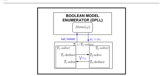
A basic architectural schema of SMT (T1∪ T2) via N.O. is described in Figure 3. (Here
BOOLEAN MODEL ENUMERATOR (DPLL) Atoms(ϕ) µ1∪ µ2 sat/unsat W eij T1-solver T1-deduce T1-solve T2-solve T2-deduce T2-solver T1∪ T2-solver
Fig. 3 A basic architectural schema of SMT (T1∪ T2) via the N.O. procedure.
16] for more details.) We assume that all Ti’s are N.O. theories and their Ti-solvers are
eij-deduction complete (see §3.2).
We consider first the case in which both theories are convex. The combined T1∪ T2-solver
receives from DPLL a pure set of literals µ, and partitions it into µT1∪ µT2, s.t. µTi is i-pure, and feeds each µTi to the respective Ti-solver. Each Ti-solver, in turn:
(i) checks the Ti-satisfiability of µTi,
(ii) deduces all the interface equalities deriving from µTi,
(iii) passes them to the other T -solver, which adds it to his own set of literals. This process is repeated until either one Ti-solver detects inconsistency (µ1∪ µ2 is
T1∪T2-unsatisfiable), or no more eij-deduction is possible (µ1∪µ2is T1∪T2-satisfiable).
In the case in which at least one theory is non-convex, the N.O. procedure becomes more complicated, because the two solvers need to exchange arbitrary disjunctions of interface equalities. As each Ti-solver can handle only conjunctions of literals, the disjunctions must be managed by means of case splitting and of backtrack search. Thus, in order to check the consistency of a set of literals, the combined T1∪ T2-solver
must internally explore a number of branches which depends on how many disjunctions of equalities are exchanged at each step: if the current set of literals is µ, and one of the Ti-solver sends the disjunction
Wn
k=1(eij)k to the other, the latter must further investigate up to n branches to check the consistency of each of the µ ∪ {(eij)k} sets separately.
4.2 Discussion
N.O. procedure was originally conceived to combine decision procedures on sets of
literals, much before the lazy SMT approach was conceived, so that it was not tailored
for interfacing with a SAT solver and for exploiting its full power. In what follows we analyze, with the help of of a few examples, the behaviour of N.O. procedure when used within a lazy SMT context, with both convex and non-convex theories.
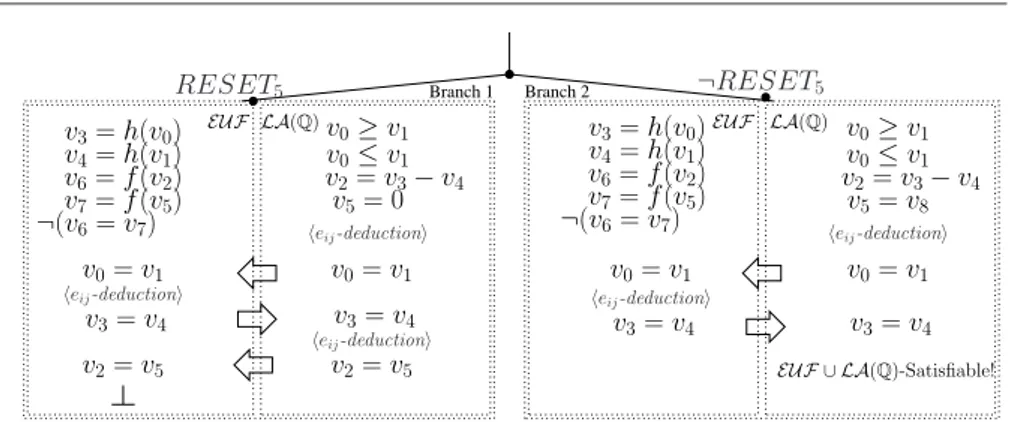
Branch 1 Branch 2 ¬RESET5 v0= v1 v2= v5 v3= h(v0) v4= h(v1) v6= f (v2) v7= f (v5) v3= v4 ¬(v6= v7) v0≥ v1 v5= 0 v0= v1 v2= v5 v3= v4 v2= v3− v4 v0≥ v1 v5= v8 v0≤ v1 v0= v1 v3= v4 v2= v3− v4 v3= h(v0) v4= h(v1) v6= f (v2) v7= f (v5) v0= v1 v3= v4 ¬(v6= v7) v0≤ v1 LA(Q) EUF ∪ LA(Q)-Satisfiable!
EUF EUF LA(Q)
heij-deductioni
heij-deductioni heij-deductioni
heij-deductioni
heij-deductioni
RESET5
Fig. 4 Search tree for the formula of Example 6.
4.2.1 Returning “eij-unaware” conflict clauses
First, in the above schema the DPLL solver is not made aware of the interface equalities
eij, so that the latter cannot occur in conflict clauses. Therefore, in order to construct the T1∪ T2-conflict clause, it is necessary to resolve backwards the last conflict clause
with (the deduction clauses corresponding to) the eij-deductions performed by each
Ti-solver. This causes the generation of possibly very long and lowly-informative con-flict(ing) clauses.
Example 5 Consider the scenario of the left branch in Example 6 and Fig. 4. Starting from the final EUF conflict, and resolving backwards wrt. the deductions performed, it is possible to obtain a final EUF ∪ LA(Q)-conflict clause as follows:
EUF-conflict : ((v6= f (v2)) ∧ (v7= f (v5)) ∧ ¬(v6= v7) ∧ (v2= v5)) → ⊥ LA(Q)-deduction : ((v2= v3− v4) ∧ (v5= 0) ∧ (v3= v4)) → (v2= v5) EUF-deduction : ((v3= h(v0)) ∧ (v4= h(v1)) ∧ (v0= v1)) → (v3= v4) LA(Q)-deduction : ((v0≥ v1) ∧ (v0≤ v1)) → (v0= v1) =⇒ EUF ∪ LA(Q)-conflict : ((v6= f (v2)) ∧ (v7= f (v5)) ∧ ¬(v6= v7) ∧ (v2= v3− v4)∧ (v5= 0) ∧ (v3= h(v0)) ∧ (v4= h(v1)) ∧ (v0≥ v1)) → ⊥.
Notice that the novel conflict clause provides no help to avoid repeating the two eij -deduction steps in the right branch in Fig. 4. ¦ 4.2.2 No learning from eij-reasoning
Second, the conflict(ing) clauses above cannot provide any information about the theory-combination steps performed by the T1∪ T2-solver. Thus, in future branches, if
run on very similar set of of literals, the combined T1∪ T2-solver may have to repeat
part or all the same eij-deduction steps.
Example 6 Consider the following pure EUF ∪ LA(Q)-formula ϕ:
EUF : (v3= h(v0)) ∧ (v4= h(v1)) ∧ (v6= f (v2)) ∧ (v7= f (v5))∧
LA(Q) : (v0≥ v1) ∧ (v0≤ v1) ∧ (v2= v3− v4) ∧ (RESET5→ (v5= 0))∧
Both : (¬RESET5→ (v5= v8)) ∧ ¬(v6= v7).
v0, v1, v2, v3, v4, v5are interface variables, v6, v7, v8are not. (Thus, e.g., (v0= v1) is
an interface equality, whilst (v0= v6) is not.) RESET5 is a Boolean variable.
Consider the search tree in Fig. 4. After the first run of unit-propagations, assume DPLL selects the literal RESET5, resulting in the assignment µdef= µEUF ∪ µLA(Q) s.t.
µEUF = {(v3= h(v0)), (v4= h(v1)), (v6= f (v2)), (v7= f (v5)), ¬(v6= v7)}
µLA(Q)= {(v0≤ v1), (v0≥ v1), (v2= v3− v4), (v5= 0)}, (5)
which propositionally satisfies ϕ. Now, the set of literals µEUF is given to the EUF-solver, which reports its consistency and deduces no new interface equality. Then the set µLA(Q) is given to the LA(Q)-solver, which reports consistency and deduces the interface equality v0 = v1, which is passed to the EUF-solver. The new set µEUF ∪
{(v0= v1)} is still EUF-consistent, but this time the EUF-solver can deduce from it
the equality (v3 = v4), which is in turn passed to the LA(Q)-solver, which deduces
(v2= v5). The EUF-solver is then invoked again to check the EUF-consistency of the
assignment µEUF ∪ {(v0 = v1), (v2 = v5)}: since this check fails, the Nelson-Oppen
procedure reports the EUF ∪ LA(Q)-unsatisfiability of the whole assignment µ. At this point, then, DPLL backtracks and tries assigning false to RESET5, 10
resulting in the new assignment µ0def= µEUF ∪ µ0LA(Q) s.t.
µEUF = {(v3= h(v0)), (v4= h(v1)), (v6= f (v2)), (v7= f (v5)), ¬(v6= v7)}
µ0LA(Q)= {(v0≤ v1), (v0≥ v1), (v2= v3− v4)(v5= v8)}, (6)
which is found EUF ∪ LA(Q)-satisfiable with a similar process (see Fig. 4), in which the eij-deductions of (v0= v1) and (v3= v4) have to be performed again. ¦
4.2.3 Forcing internal case-splits in non-convex theories
Third, in case of non-convex theories, the combined T1∪ T2-solver must handle
inter-nally the case-splits caused by the fact that each Ti-solver may receive from the other disjunctions of interface equalities.
Example 7 Consider the conjunction of literals µdef= µEUF∧ µLA(Z)(2) of Example 1:
µEUF : ¬(f (v1) = f (v2)) ∧ ¬(f (v2) = f (v4)) ∧ (f (v3) = v5) ∧ (f (v1) = v6)∧
µLA(Z): (v1≥ 0) ∧ (v1≤ 1) ∧ (v5= v4− 1) ∧ (v3= 0) ∧ (v4= 1)∧
(v2≥ v6) ∧ (v2≤ v6+ 1).
(7)
Here all the variables (v1, . . . , v6) are interface ones. µ contains only unit clauses, so
after the first run of unit-propagations, DPLL generates the assignment µ which is simply the set of literals in µ. One possible run of the N.O. procedure is depicted in Fig. 5.11
First, the sub-assignment µEUF is given to the EUF-solver, which reports its con-sistency and deduces no interface equality. Then, the sub-assignment µLA(Z) is given
10 We assume that DPLL adopts the last UIP strategy using the T -conflict clause described
in Example 5. Other strategies may lead to propagate also ¬(v5 = 0) in the right branch,
which would not affect the result.
11 Notice that there may be different runs depending on the order in which the e
ij-deductions
v1
≥ 0
v1
≤ 1
v2
≥ v6
v2
≤ v6
+ 1
v4
= 1
v3
= 0
v5
= v
4− 1
¬(f (v2
) = f (v
4))
f (v3
) = v
5f (v1
) = v
6¬(f (v1
) = f (v
2))
v2
= v
3v1
= v
4v1
= v
3v5
= v
6v2
= v
4v2
= v
3∨ v2
= v
4v
1= v
3∨ v
1= v
4v5
= v
6v3
= v
5v
3= v
5µ
LA(Z)LA(Z)
µ
EUFEUF
EUF ∪ LA(Z)-Satisfiable! heij-deductioni heij-deductioni heij-deductioni heij-deductioniFig. 5 The N.O. search tree for the formula of Example 7
to the LA(Z)-solver, which reports its consistency and deduces first (v3 = v5) and
then the disjunction (v1 = v3) ∨ (v1 = v4), which are both passed to the
EUF-solver. Whilst the first produces no effect, the second forces a case-splitting so that the two equalities (v1= v3) and (v1= v4) must be analyzed separately by the
EUF-solver. The first branch, corresponding to selecting (v1 = v3), is opened: then the
set µEUF ∪ {(v1 = v3)} is EUF-consistent, and the equality (v5 = v6) is deduced.
After that, the assignment µLA(Z)∪ {(v5= v6)} is passed to the LA(Z)-solver, that
reports its consistency and deduces another disjunction, (v2= v3) ∨ (v2= v4). At this
point, another case-splitting is needed in the EUF-solver, resulting in the two branches
µEUF ∪ {(v1= v3), (v2 = v3)} and µEUF∪ {(v1= v3), (v2= v4)}. Both of them are
found inconsistent, so the whole branch previously opened by the selection of (v1= v3)
is found inconsistent.
At this point, the other case of the branch (i.e. the equality (v1= v4)) is selected,
and since the assignment µEUF∪ {(v1= v4)} is EUF-consistent and no new interface
equality is deduced, the N.0. method reports the EUF ∪ LA(Z)-satisfiability of µ. ¦ 4.2.4 Requiring eij-deduction complete Ti-solvers
Finally, as highlighted from the two previous examples, the ability of the Ti-solvers to carry out eij-deductions (see §3.2) is crucial: each solver must be eij-deduction complete, that is, it must be able to derive the (disjunctions of) interface equalities eij which are entailed by its current facts µTi. As highlighted in §3.2, for some theories this operation can be very expensive.
5 SMT for combined theories via the DTC procedure
Delayed Theory Combination (DTC) is a more recent general-purpose procedure for
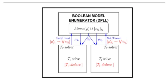
BOOLEAN MODEL ENUMERATOR (DPLL) [µ0 T1→ W eij] [µ0T2→ W eij] [T1-deduce ] [T2-deduce ] µe µT2 µT1 Sat/Unsat Sat/Unsat Atoms(ϕ) ∪ {eij}ij T1-solve T2-solve T1-solver T2-solver
Fig. 6 A basic architectural schema of SMT (T1∪ T2) via the DTC procedure.
DTC works by performing Boolean reasoning on interface equalities, possibly combined with T -propagation, with the help of the embedded DPLL solver. As with N.O. proce-dure, DTC is based on the N.O. logical framework of §2.2, and thus considers signature-disjoint stably-infinite theories with their respective Ti-solvers, and pure input formulas (although most of the considerations on releasing purity and stably-infiniteness in §2.2 hold for DTC as well). Importantly, no assumption is made about the eij-deduction capabilities of the Ti-solvers (§3.2): for each Ti-solver, every intermediate situation from complete eij-deduction to no eij-deduction capabilities is admitted.
5.1 The DTC procedure
A basic architectural schema of DTC is described in Figure 6. In DTC, each of the two Ti-solvers interacts directly and only with the Boolean enumerator (DPLL), so that there is no direct exchange of information between the Ti-solvers. The Boolean enumerator is instructed to assign truth values not only to the atoms in Atoms(ϕ), but also to the interface equalities eij’s. Consequently, each assignment µp enumerated by DPLL is partitioned into three components µpT
1, µ p T2 and µ
p
e, s.t. each µTi is the set of
i-pure literals and µe is the set of interface (dis)equalities in µ, so that each µTi∪ µe is passed to the respective Ti-solver.
An implementation of DTC [9,10] is based on the online schema of Figure 1 in
§3.1, exploiting early pruning, T -propagation, T -backjumping and T -learning. Each
of the two Ti-solvers interacts with the DPLL engine by exchanging literals via the assignment µ in a stack-based manner. The T -DPLL algorithm of Figure 1 in §3.1 is modified to the following extents:
1. T -DPLL is instructed to assign truth values not only to the atoms in ϕ, but also to
2. T -decide next branch is modified to select also interface equalities eij’s not oc-curring in the formula yet12, but only after the current assignment propositionally satisfies ϕ.
3. T -deduce is modified to work as follows: instead of feeding the whole µ to a
(com-bined) T -solver, for each Ti, µTi∪ µe, is fed to the respective Ti-solver. If both return sat, then T -deduce returns sat, otherwise it returns Conflict.
4. T -analyze conflict and T -backtrack are modified so that to use the conflict set
returned by one Ti-solver for T -backjumping and T -learning. Importantly, such conflict sets may contain interface (dis)equalities.
5. Early-pruning and T -propagation are performed. If one Ti-solver performs the eij -deduction µ∗|=Ti
Wk
j=1ej s.t. µ∗ ⊆ µTi∪ µe and each ej is an interface equality, then the deduction clause T 2B(µ∗→Wkj=1ej) is learned.
6. [If and only if both Ti-solvers are eij-deduction complete.] If an assignment
µ which propositionally satisfies ϕ is found Ti-satisfiable for both Ti’s, and neither
Ti-solver performs any eij-deduction from µ, then T -DPLL stops returning sat.13 In order to achieve efficiency, other heuristics and strategies have been further suggested in [9,10], and more recently in [18,14].
In short, in DTC the embedded DPLL engine not only enumerates truth assign-ments for the atoms of the input formula, but it also assigns truth values for the interface equalities that the T -solver’s are not capable of inferring, and handles the case-split induced by the entailment of disjunctions of interface equalities in non-convex theories. The rationale is to exploit the full power of a modern DPLL engine and to delegate to it part of the heavy reasoning effort on interface equalities previously due to the Ti-solvers.
5.2 Discussion
DTC has been conceived in such a way to fully exploit the power of DPLL within a lazy SMT framework. We analyze the behaviour of DTC with the help of the examples we used in §4.2 for N.O., considering both the case in which the Ti-solvers are eij-deduction complete and the case in which the Ti-solvers have no eij-deduction capability, with both convex and non-convex theories.
In all the following examples we assume that DTC adopts the “N.O.-mimicking strategy” of Fig. 11, which will be discussed in §6. Moreover, in order to simplify the explanation and to introduce some concepts which will elaborated in §6, in both examples 8 and 10 (Ti-solvers with no eij-deduction capability) we will assume that both Ti-solver always return ¬eij-minimal conflict sets.
Notationally, µ0T i, µ
00 Ti, µ
000
Ti denote generic subsets of µTi and “Cij” denotes either the T -deduction clause causing the T -propagation of (vi= vj) or the conflicting clause causing the backjump to (vi = vj). For better readability, we represent directly the assignment to T -atoms rather than to their Boolean abstraction (e.g., we say “assign
¬(v5= 0)” instead of “assign ¬Bi” s.t. Bidef= T 2B((v5= 0))).
12 Notice that an interface equality occurs in the formula after a clause containing it is
learned, see point 4..
13 This is identical to the T
....
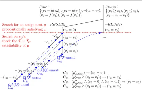
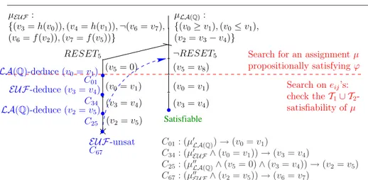
LA(Q)-unsat C01 C01: (µ0LA(Q)) → (v0= v1) C34: (µ0EUF∧ (v0= v1)) → (v3= v4) C25: (µ00LA(Q)∧ (v5= 0) ∧ (v3= v4)) → (v2= v5) C67: (µ00EUF∧ (v2= v5)) → (v6= v7) ¬(v3= v4) ¬(v2= v5) (v3= v4) (v2= v5) C67 C25 C34 ¬e0 ij LA(Q)-unsat (v0= v1) (v5= 0) EUF-unsat ¬RESET5 (v5= v8) ¬(v0= v1) ¬eij” EUF-unsat µLA(Q): {(v0≥ v1), (v0≤ v1), (v2= v3− v4)} µEUF: {(v3= h(v0)), (v4= h(v1)), ¬(v6= v7), (v6= f (v2)), (v7= f (v5))}Search for an assignment µ propositionally satisfying ϕ
Search on eij’s:
check the T1∪ T2
-satisfiability of µ
RESET5
Fig. 7 DTC execution of the first branch of Example 8, with no eij-deduction. Here we
assume that all conflict sets returned by the Ti-solvers are ¬eij-minimal.
5.2.1 Delaying theory combination
First, due to point 2. above, the Boolean search tree is divided into two parts: the top part, performed on the atoms currently occurring in the formula, in which a (par-tial) truth assignment µ propositionally satisfying ϕ is searched, and the bottom part, performed on the eij’s which do not yet occur in the formula, in which the T1∪ T2
-satisfiability of µ is checked by building a candidate arrangement µe. Thus, in every branch the reasoning on eij’s is not performed until (and unless) it is strictly neces-sary. (From which the name “Delayed Theory Combination”.) E.g., if in one branch
µ is such that one µTi component is Ti-unsatisfiable, no Boolean reasoning on eij’s is performed.
To this extent, it is important to exploit the issue of partial assignments [36]: when the current partial assignment µ propositionally satisfies the input formula ϕ, the remaining atoms occurring in ϕ can be ignored and only the new eij’s are then selected. Importantly, if µ is a partial assignment, then it is sufficient that µeassigns only the eij’s which have an actual interface role in µ. (E.g., if µ is partial and v is an interface variable in ϕ but it occurs in no 1-pure literal in µ, then v has no “interface role” for µ, so that every interface equality containing v can be ignored by µe. )
Example 8 Consider again the EUF ∪ LA(Q)-formula ϕ (4) of Example 6:
EUF : (v3= h(v0)) ∧ (v4= h(v1)) ∧ (v6= f (v2)) ∧ (v7= f (v5))∧
LA(Q) : (v0≥ v1) ∧ (v0≤ v1) ∧ (v2= v3− v4) ∧ (RESET5→ (v5= 0))∧
Both : (¬RESET5→ (v5= v8)) ∧ ¬(v6= v7).
(8) and consider the assignment µ (5) obtained after T -DPLL assigns RESET5and
unit-propagates (v5 = 0). Let µ be partitioned into µLA(Q) and µEUF as in Fig. 7. µ propositionally satisfies ϕ (µ |=p ϕ), and µ is a partial assignment because it does not assign (v5 = v8). By a call to the Ti-solvers, both µLA(Q) and µEUF are found
consistent in the respective theories. Thus, in order to check the T1∪ T2-consistency of
µ, T -DPLL generates and explores a Boolean search sub-trees on the eijs according to the Strategy of Figure 11.
First T -DPLL starts selecting (the negated value of) the new eij’s, each time invoking incrementally the Ti-solvers (EP), until it selects ¬(v0= v1), which causes a
LA(Q) conflict. As LA(Q) is convex and LA(Q)-Solver is ¬eij-minimal, it returns a conflict set in the form µ0LA(Q)∪ {¬(v0= v1)} s.t. {(v0≥ v1), (v0≤ v1)} ⊆ µ0LA(Q)⊆
µLA(Q). Thus DTC learns the corresponding clause C01 and backjumps up to µ (or
even higher), hence unit propagating (v0= v1).
What happens next depends on whether the learned clause C01 contains the
re-dundant LA(Q) atom (v5= 0) or not. Here we consider the “worst” case, when such
atom occurs in C01. This means that DTC backjumps after the unit-propagation of
(v5 = 0) 14. Then (v0 = v1) is unit-propagated and new unassigned ¬eij’s are se-lected again, until ¬(v3 = v4) generates another conflict represented by clause C34,
which causes backjumping and unit-propagating (v3= v4). The same is repeated for
(v2= v5). Then µ∪{(v0= v1), (v3= v4), (v2= v5)} is found EUF-inconsistent s.t. the
conflict is represented by the clause C67, and the whole procedure backtracks, causing
the unit-propagation of ¬RESET5 and (v5= v8).
Then the search proceeds from here, with the benefit that T -DPLL can reuse the clauses C01-C67to avoid repeating research performed in the previous branch, as
explained below.
¦ 5.2.2 Learning from eij reasoning
Second, thanks to points 1., 2., 4. and 5., the interface equalities eij’s are included in the conflict(ing) and deduction clauses derived by T -conflicts and T -deduction. Therefore, instead of one long eij-free T1∪T2-conflict clause, it is possible to learn a bunch of (much
shorter) conflict and deduction clauses corresponding to the conflicts and deductions returned by the Ti-solvers. Moreover, the reasoning steps on eij’s which are performed in order to decide the T1∪ T2-consistency of one branch µ (both Boolean search on
eij’s and eij-deduction steps) are saved in the form of clauses and thus they can be reused to check the T1∪ T2-consistency of all subsequent branches. This allows from
pruning search and prevents redoing the same search/deduction steps from scratch.
Example 9 Consider again the EUF ∪ LA(Q) formula ϕ of Examples 6 and 8. Figure 8 illustrates a DTC execution when both Ti-solvers are eij-deduction complete (that is, under the same hypotheses as N.O.). As before, we assume T -DPLL adopts Strategy 1 of Fig. 11.
On the left branch (when RESET5is selected), after (v5= 0) is unit-propagated,
the LA(Q)-solver deduces (v0 = v1), and thus the deduction clause C01 is learned
and (v0= v1) is unit-propagated. Consequently, the EUF-solver can deduce (v3= v4),
causing the learning of C34and the unit-propagation of (v3= v4), which in turn causes
the LA(Q)-deduction of (v2 = v5), the learning of C25 and the unit-propagation of
(v2= v5).
14 More precisely, by Step 2. of Strategy 1, DTC eliminates (v
5 = 0) from the conflict
clause C01by resolving the latter with the clause RESET5→ (v5= 0) in ϕ, thus substituting
(v5= 0) with RESET5into the conflict clause used to drive T -backjumping. A similar process