QUASI RANDOM RESAMPLING DESIGNS FOR MULTIPLE
FRAME SURVEYS
Cherif Ahmat Tidiane Aidara1
Department of Mathematics, University of The Gambia, Brikama Campus, The Gambia
1. INTRODUCTION
Multiple frame surveys have recently received a great deal of attention from researchers (see Skinner and Rao, 1996; Lohr and Rao, 2000, 2006; Mecatti, 2007; Lohr, 2007). Al-though the initial use of multiple frame surveys was motivated by a reduction of sur-vey sampling costs (see Hartley, 1962), its current use is more geared towards address-ing frame undercoverage shortcomaddress-ings such as capturaddress-ing special, rare, and difficult-to-sample populations (see Kalton and Anderson, 1986).
In multiple frame surveys, it is assumed that the population of interest is covered adequately by a combination of sampling frames, each covering partially the population. Estimation is usually carried out by sampling independently from each of the sampling frames and creating estimators that account for units appearing in different sampling frames.
As in classical survey sampling, the standard error plays a crucial role in multiple frame survey sampling as it is used to measure the quality of survey estimators. Tech-niques to generate standard errors of survey estimators have been designed and can be put into two main categories namely the analytic techniques and the replication tech-niques. The analytic techniques include the Taylor linearization which involves differ-entiation of some functions of interest; whereas the replication techniques include the Jackknife and the bootstrap which rely solely on computation. The reader is invited to look into (see Lohr and Rao, 2000; Lohr, 2007).
Among all these standard error estimation techniques, the bootstrap is the most ad-vantageous one in that it works for both smooth and non smooth statistics; in addition, it allows the user to choose the number of replication runs needed. Statistics Canada has gradually settled into using the bootstrap technique; andR= 500 to R = 1000 sim-ulation runs are used in practice in the estimation of the standard error through the bootstrap technique (see Girard, 2009).
It is worth noting that the bootstrap method is based on Monte Carlo simulation which uses pseudo random numbers and has a convergence rate of 1/pR where R is the number of simulation runs. However, there exists a more efficient simulation technique (called quasi Monte Carlo simulation) which has a faster convergence rate 1/R and relies on quasi random numbers that are more uniformly distributed than the pseudo random numbers in the unit hypercube.
The main contribution of the present paper is that it proposes a couple of techniques that use quasi Monte Carlo simulation to generate efficient resamples for the bootstrap standard error estimation in multiple frame surveys. These techniques are inspired from Aidara (2013) and Teytaudet al. (2006).
The rest of the article is organized as follows. Section 2 gives a review of the standard Sobol sequence and at the same time presents the shuffled Sobol sequence. Section 3 presents a brief review of the multiplicity estimator. Section 4 proposes applications of quasi Monte Carlo simulation in bootstrap variance estimation of multiple frame survey estimators. Section 5 presents empirical studies that investigate the performance of the proposed techniques to the bootstrap variance estimation of the multiplicity estimator. Section 6 gives some concluding remarks.
2. THE SHUFFLEDSOBOL SEQUENCE
As the most popular and used quasi random sequence, the Sobol sequence has been studied extensively in the applied mathematics, computer science, as well as other fields of knowledge. As a consequence we only consider a brief review of the construction of the Sobol sequence and follow the presentation in Joe and Kuo (2008).
The shuffled Sobol sequence is derived from the standard Sobol sequence which is a D-dimensional sequence (where D≥ 2) that uses exclusively base two in all its dimen-sions. The construction of the shuffled Sobol sequence follows a five-step procedure. The first four steps form the standard Sobol sequence and the fifth step performs the randomization. Since these steps are identical for each of the dimensions of the Sobol sequence, the procedure for one dimension is illustrated below.
Step 1: choose an arbitrary primitive polynomial of degreeα as follows
P(x) = xα+ a1xα−1+ ··· + aα−1x+ 1 (1)
with coefficientsai∈ {0, 1}. For instance the polynomials x +1 and x2+ x +1 are primitive polynomials of degree one and two respectively.
Step 2: choose arbitrarily the set of the firstα initialization numbers
{m1,m2,· · · , mα} such that each mi is odd and less than 2i fori = 1,··· ,α; then generate the rest of the initialization numbers through the recurrence relation
whereai are the coefficients of the primitive polynomial,j> α, and ⊕ is the xor operation defined as 1⊕ 0 = 0 ⊕ 1 = 1 and 0 ⊕ 0 = 1 ⊕ 1 = 0.
Step 3: define the direction numbers by
vj=mj 2j .
This is equivalent to expressingmjin binary representation and then shifting the position of the fractional point byj places to the left.
Step 4: use the more efficient recursive algorithm in Antonov and Saleev (1979) to cal-culate the(k + 1)t hSobol number as
ψk+1= ψk⊕ v` (3)
where` is the index of the first 0 digit from the right in the binary representation ofk, v`is the`t hdirection number, andψ
0= 0 is assumed to be the starting point of the sequence.
Step 5: reshuffle randomly the generated standard Sobol numbers to obtain the shuffled Sobol sequence. 0.0 0.2 0.4 0.6 0.8 1.0 0.0 0.2 0.4 0.6 0.8 1.0
Standard Sobol Sequence 250 points 49th dimension 50th dimension 0.0 0.2 0.4 0.6 0.8 1.0 0.0 0.2 0.4 0.6 0.8 1.0
Shuffled Sobol Sequence 250 points
49th dimension
50th dimension
Figure 1 – 250 Sobol points.
It is worth noting that a distinct primitive polynomial is chosen for each dimension of the Sobol sequence.
The quality of the Sobol sequence depends on the choice of the initialization num-bers. Any improper choice of these numbers leads to high correlations between different
dimensions of the Sobol sequence (see left hand side plot of Figure 1). Fortunately, ta-bles of good initialization numbers together with primitive polynomials are available in the literature (for more details, see Joe and Kuo, 2008).
The shuffled Sobol sequence is contrasted with the standard Sobol sequence in Fig-ure 1. It is obvious that the shuffled Sobol sequence displays a more uniform distribution than the standard Sobol sequence in high dimension (see right hand side plot of Figure 1). 3. REVIEW OF THE MULTIPLICITY ESTIMATOR
Suppose our population of interestU which consists of N units is adequately covered byQ(≥ 2) overlapping sampling frames each of size N(q) and denoted byA(q) where q = 1,··· ,Q. The frames divide naturally the population of interest into 2Q− 1 non overlapping domains. The majority of estimators in multiple frame surveys are based on these non overlapping domains (see, e.g., Halton, 1960; Skinner and Rao, 1996). However Mecatti (2007) proposed a new approach that does not make use of these non overlapping domains. This approach makes use of a partial membership information, termedmultiplicity which is the number of frames a unit belongs. It is worth noting that unit multiplicity can be collected easily during the data collection process.
To illustrate the details of the multiplicity approach, supposeQ independent proba-bility samples each of sizen(q)and denoted byS(q)is selected fromA(q)forq= 1,··· ,Q. The probability sampling design forA(q)generates for unitk a known inclusion proba-bility,π(q)k > 0, and a corresponding sampling design weight dk(q)= 1/π(q)k . The values (yq k,mq k) of the study variable y and the multiplicity m are recorded for all k ∈ S(q). At this juncture it is worth observing that every population uniti∈ U belongs to a finite number of sampling framesmiand therefore any frame-specific unit(qk) corresponds to a uniquei∈ U . If the objective is to estimate a population total
Ty= N X
i=1 yi, then it is easy to verify that
Ty= Q X q=1 X k∈A(q) yq km−1q k.
As a result, the multiplicity estimator of the population totalTyis defined as ty= Q X q=1 X k∈S(q) dk(q)yq kmq k−1.
The estimatortyis indeed a function of weights and can thus be expressed as ty= f d(1),· · · , d(q),· · · , d(Q),
where d(q)is the vector of weights from frameq. 4. THE PROPOSED ALGORITHMS
This section presents two algorithms that generate efficiently independent bootstrap samples for multiple frame surveys while using quasi random sequences. These algo-rithms are applicable to all multiple frame survey estimators. A notation similar to the one used in Lohr and Rao (2006) is adopted throughout the rest of the paper.
LetA(1),· · · , A(Q) be theQ overlapping sampling frames that cover adequately the population of interest. Let A(q), q = 1,··· ,Q be partitioned into H(q) nonoverlap-ping strataA(q)=¦A(q)1 ,· · · , A(q)H(q)
©
, whereA(q)h is comprised ofNh(q) primary sampling units (psu). Let S(1),· · · , S(Q) beQ independent samples drawn respectively from the Q frames. A probability sample Sh(q)is selected from theh-th stratum of the q-th sam-pling frameA(q)h . The probability sampling design generates for psui within the h-th stratum of theq-th sampling frame a known inclusion probability,π(q)hi > 0, and a cor-responding sampling designdhi(q)= 1/π(q)hi. It is worth noting thatSh(q)= {1,2,··· , n(q)h }, S(q)= SHh=1(q)Sh(q), andn(q)= PH(q)
h=1n(q)h is the size ofS(q).
The first proposed algorithm works generally in the following manner. First, a Sobol sequence ofD= PQq=1H(q)dimensions is generated. Then, the firstH(1)components of the Sobol sequence are mapped to theH(1)strata of the sampleS(1)on a one-to-one basis, the nextH(2)components of the Sobol sequence are mapped to theH(2)strata of the sampleS(2)on a one-to-one basis, and so on. It is worth noting that the Sobol sequence elements are mapped through the quantile function of the binomial distribution.
For a detailed illustration of the proposed algorithm, suppose a bootstrap sample Sh∗(q)is drawn fromSh(q)by sampling with replacement for h = 1,2,··· , H(q) indepen-dently. Sampling with replacement the units of Sh(q) ensures a selection probability of 1/n(q)h for each unit. If x(q)hi denotes the number of times unit i of stratum h ap-pears in the bootstrap sample Sh∗(q) and m(q)h (≤ n(q)h ) the number of draws, then Sh∗(q) can be represented as
§
x(q)h1,· · · , x(q) hnh(q)
ª
which has a multinomial distribution with size m(q)h = Pn
(q) h
i=1x(q)hi and cell probabilities p (q) hi = 1/n
(q)
h . It is worth noting that eachx (q) hi is binomially distributed with sizem(q)h and probability phi(q). In addition, ifi− 1 units have already been observed, then thei-th unit xhi(q)has a binomial distribution with size m(q)h −Pi−1 j=1xh j(q)and probability p (q) hi / 1−Pi−1 j=1p(q)h j .
The bootstrap sampleSh∗(q)is generated by mapping the elements of theh-th com-ponent of theH(q)components of the Sobol sequence to the units ofSh(q)as shown in
the following procedure.
1. Generateψ(q)h1 from theh-th dimension of the Sobol sequence. 2. Definex(q)h1 minimal such that
Dψ(q) h1 = inf¦x (q) h1 :ψ (q) h1 ≤ Prob Xh1(q)≤ x(q)h1©whereXh1(q)is binomially distributed with sizem(q)h and probabilityp(q)h1.
3. Fori= 2 to nh(q)
1. Generateψ(q)hi from theh-th dimension of the Sobol sequence. 2. Definexhi(q)minimal such that
Dψ(q)hi = inf¦x(q)hi :ψ(q)hi ≤ ProbXhi(q)≤ x(q)hi© whereXhi(q) is binomially distributed with sizemh(q)−Pi−1
j=1xh j(q)and probabilityp (q) hi/ 1−Pi−1 j=1ph j(q) . 4. Repeat steps 1 to 3 for h= 1,··· , H(q) to obtain the bootstrap sample from the
stratified sampleS∗(q)= SH(q) h=1S∗(q)h
5. Repeat steps 1 to 4 forq= 1,··· ,Q to obtain the bootstrap sample for the multiple frame survey.
The second proposed algorithm uses a Sobol sequence whose dimension is equal to the number of sampling frames i.e. D= Q. In this method, the first component of the Sobol sequence is mapped to the elements of the sample drawn from the first sampling frame, the second component of the Sobol sequence is mapped to the elements of the sample drawn from the second sampling frame, and so on. The details of the mapping are presented in the following algorithm:
1. Generateψ(q)h1 from theq-th dimension of the Sobol sequence. 2. Definex(q)h1 minimal such that
Dψ(q)h1 = inf¦x(q)h1 :ψ(q)h1 ≤ ProbXh1(q)≤ x(q)h1©whereXh1(q)is binomially distributed with sizem(q)h and probabilityp(q)h1.
3. Fori= 2 to nh(q)
1. Generateψ(q)hi from theq-th dimension of the Sobol sequence. 2. Definexhi(q)minimal such that
Dψ(q)hi = inf¦x(q)hi :ψ(q)hi ≤ ProbXhi(q)≤ x(q)hi© whereXhi(q) is binomially distributed with sizemh(q)−Pi−1
j=1xh j(q)and probabilityp (q) hi/ 1−Pi−1 j=1ph j(q) .
4. Repeat steps 1 to 3 for h= 1,··· , H(q) to obtain the bootstrap sample from the stratified sampleS∗(q)= SH(q)
h=1S∗(q)h . Notice that the firstn (q)
1 elements of the Sobol sequence are used for the first stratum ofS∗(q)that isS∗(q)
1 , the secondn (q)
2 elements of the Sobol sequence are used for the second stratum ofS∗(q)that isS∗(q)
2 , and so on.
5. Repeat steps 1 to 4 forq= 1,··· ,Q to obtain the bootstrap sample for the multiple frame survey.
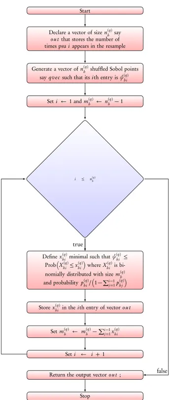
At this juncture, it is befitting to present both a flowchart and an example that illus-trate the use of these algorithms. Since the algorithms are similar, only a flowchart for the first algorithm from steps 1 to 3 is presented and captured in Figure 2.
As for the example, consider the population in Table 1 where the column names are uid, h, i, y represent respectively the unique identity number of the element, the stratum, the relative number of the stratum element, some parameter of interest. Without loss of generality,Q(= 2) overlapping frames (as in Tables 2, 3) with H(1)= H(2)(= 2) strata are selected from the population independently. Notice that a further column denoted m is added in these tables to specify whether or not the element is only captured in one frame or both. Consider further that two stratified samplesS(1)andS(2)are selected independently, using the sampling package (Tillé and Matei, 2016), from the frames such that S(1) = S1(1)∪ S2(1) and S(2)= S1(2)∪ S2(2). Suppose we selected five elements inS1(1) and four elements in S2(1); three elements inS2(2) and four elements inS2(2). Using the uid, the selected elements are as followsS1(1)= {1,3,5,10,11} and S2(1)= {16,32,34,35} from the first and second stratum of the first frame; and S1(2) = {8,9,10} and S2(2) = {19, 20, 24, 27} from the first and second stratum of the second frame. From the first proposed algorithm, we have to generate a reshuffled Sobol sequence of 4 dimensions and use the first 2 dimensions for the resampleS∗(1)and the remaining 2 dimensions for the resample S∗(2). Upon applying this algorithm, we have obtained the following stratum resamples S1∗(1) = {1,0,1,0,2}, S2∗(1) = {1,1,0,1}, and S1∗(2) = {0,1,1}, S2∗(2) = {0, 1, 1, 1}. The numbers in the stratum resample should be understood as the number of times the corresponding elements are selected.
From the second proposed algorithm, we have to generate a reshuffled Sobol se-quence of 2 dimensions and use the elements in the first dimension for the resample S∗(1) and the elements in the second dimension for the resampleS∗(2). In details, we first generate a sequence of length n(1)= n(1)1 + n(1)2 in the first dimension. Then we use the firstn1(1)points for the first stratum and the nextn2(1)points for the second stra-tum. The same approach is used for the resampleS∗(2). Upon applying this algorithm, we have obtained the following stratum resamplesS1∗(1)= {1,0,1,0,2}, S2∗(1)= {1,1,1,0} andS1∗(2)= {1,1,0}, S2∗(2)= {2,0,0,1}.
Start
Declare a vector of sizen(q)h say ou t that stores the number of times psui appears in the resample
Generate a vector ofn(q)h shuffled Sobol points sayq v e c such that its ith entry isψ(q)hi
Seti ← 1 and mh(q) ← n(q)h − 1
i ≤ n(q)h
Definex(q)
hi minimal such thatψ (q) hi ≤
ProbXhi(q)≤ x(q)hiwhereXhi(q)is bi-nomially distributed with sizem(q)h and probabilityp(q)hi/
1−Pi−1 j=1p(q)h j
Storex(q)
hi in theith entry of vector ou t
Setm(q)h ← m(q)h −Pi−1 j=1x(q)hi
Seti ← i + 1
Return the output vectorou t ;
Stop true
false
TABLE 1
A toy population from which two overlapping frames are extracted.
uid h i y 1 1 1 1.693 2 1 2 1.980 3 1 3 0.904 4 1 4 0.536 5 1 5 0.990 6 1 6 2.147 7 1 7 1.014 8 1 8 0.895 9 1 9 1.918 10 1 10 1.302 11 1 11 3.667 12 1 12 0.150 13 1 13 1.059 14 1 14 3.100 15 1 15 3.503 16 2 1 3.187 17 2 2 0.456 18 2 3 1.389 19 2 4 2.466 20 2 5 2.923 21 2 6 1.546 22 2 7 6.133 23 2 8 0.848 24 2 9 1.003 25 2 10 1.677 26 2 11 3.040 27 2 12 3.444 28 2 13 1.781 29 2 14 5.052 30 2 15 0.530 31 2 16 1.690 32 2 17 0.970 33 2 18 1.660 34 2 19 0.755 35 2 20 1.817
TABLE 2
First frame extracted from the toy population.
uid h i y m 1 1 1 1.693 1 2 1 2 1.980 2 3 1 3 0.904 1 4 1 4 0.536 2 5 1 5 0.990 2 7 1 6 1.014 1 10 1 7 1.302 2 11 1 8 3.667 1 13 1 9 1.059 1 14 1 10 3.100 1 16 2 1 3.187 2 17 2 2 0.456 1 20 2 3 2.923 2 25 2 4 1.677 2 26 2 5 3.040 1 28 2 6 1.781 2 29 2 7 5.052 2 31 2 8 1.690 1 32 2 9 0.970 1 34 2 10 0.755 1 35 2 11 1.817 2
TABLE 3
Second frame extracted from the toy population.
uid h i y m 2 1 1 1.980 2 4 1 2 0.536 2 5 1 3 0.990 2 6 1 4 2.147 1 8 1 5 0.895 1 9 1 6 1.918 1 10 1 7 1.302 2 12 1 8 0.150 1 15 1 9 3.503 1 16 2 1 3.187 2 18 2 2 1.389 1 19 2 3 2.466 1 20 2 4 2.923 2 21 2 5 1.546 1 22 2 6 6.133 1 23 2 7 0.848 1 24 2 8 1.003 1 25 2 9 1.677 2 27 2 10 3.444 1 28 2 11 1.781 2 29 2 12 5.052 2 30 2 13 0.530 1 33 2 14 1.660 1 35 2 15 1.817 2
It is worth noting that the second algorithm presents an advantage over the first one in that the dimension of the Sobol sequence is reduced significantly. Knowing that quasi random sequences present a better uniform distribution of their elements in low dimension, the results from this algorithm are expected to be more accurate.
Then the extended Rao-Wu bootstrap weight for the frames proposed in Lohr (2007) was used to compute the variance. Supposedhi(q)is the weight attached to uniti of stra-tum h for the q-th sampling frame. Then the corresponding bootstrap weight for the b -th simulation run is denoted by dhi(q)[b] and defined as
dhi(q)[b] = dhi(q)n (q) h m(q)h x (q) hi [b],
wherexhi(q)[b] is the number of times unit i of stratum h is selected in the b-th simulation run.
To estimate the bootstrap variance of an estimator sayt , the separated and combined bootstrap approaches proposed in Lohr (2007) are used. For the separated bootstrap approach,Bq bootstrap samples are created from the sampleS(q)of theq-th frame Aq using the above algorithm. For each of theH(q)dimensions associated with the sample S(q),Bqnh(q)elements are generated and the firstn(q)h elements are used for the creation of the h-th stratum of the first bootstrap sample Sh∗(q)[1], the next n(q)h elements are used for the creation of the h-th stratum of the second bootstrap sample Sh∗(q)[2], and so on. Therefore, theb -th bootstrap sample is defined as S∗(q)[b] = SH(q)
h=1Sh∗(q)[b]. The separated bootstrap method is estimated by
vs= Q X q=1 1 Bq Bq X b=1 (tq y[b] − ty)2. (4)
Note thattyq[b] = f (d(1),· · · , d(q)[b],··· ,d(Q)) which means that the original weights inS(q)are replaced by the bootstrap weights for just the frameq in the b -th simulation run
For the combined bootstrap approach,B bootstrap samples are created from the sample S(q)of theq-th frame Aq using the above algorithm. For each of theH(q) di-mensions associated with the sample S(q), B n(q)h elements are generated and the first n(q)h elements are used for the creation of the h-th stratum of the first bootstrap sam-pleS∗(q)h [1], the next n(q)h elements are used for the creation of theh-th stratum of the second bootstrap sampleS∗(q)h [2], and so on. Therefore, the b-th bootstrap sample is
defined asS∗(q)[b] = SH(q)
h=1Sh∗(q)[b]. The combined bootstrap method is given by vc= 1 B B X b=1 (ty[b] − ty)2. (5)
Note thatty[b] = f (d(1)[b],··· ,d(q)[b],··· ,d(Q)[b]) which means that in the b-th sim-ulation run, the original weights in theQ frames are simultaneously replaced by the bootstrap weights from theQ independent samples.
For the second algorithm, the method works as follows. For theq-th dimension, Bqn(q)elements are generated and the firstn(q)elements are used for the creation of the first bootstrap sample. The nextn(q)elements are used for the creation of the second bootstrap sample and so on. It is worth noting that the size ofS(q)isn(q)= PH(q)
h=1n(q)h and that the b -th bootsrap sample is obtained by using the first n1(q) elements of the sequence for the sampling of the units of the first stratum ofS(q), the nextn2(q)elements of the sequence for the sampling of the units of the second stratum ofS(q), and so on. 5. SIMULATION STUDY
A limited simulation study was carried out to investigate the performance of the pro-posed methods in a three-frame setup. Each of the six different stratified finite popula-tions described in Chen and Sitter (1999) was used in some preliminary simulapopula-tions. For each population, we created three overlapping frames and tested the proposed methods; and there were no significant differences in the performance of the proposed methods. Hence we decided to report the results of our simulation study using only one of these six populations namely population 2 of Chen and Sitter (1999). As a reminder, popula-tion 2 hadH= 4 strata with stratum sizes Nh= 8000 − 300h for h = 1,2,3,4. For the ith unit within the hth stratum, the characteristics xhiwere generated by addingh/2 to χ2
2hvariate and theyhi were generated using the model
yhi= αh+ βhxhi+ γhxhi2 + ξhxahiεhi (6) for specific values ofαh,βh,γh,a andξh, whereεhi are random variables, independent and identically distributed overi, from a chi-square distribution with bhdegrees of free-dom,χ2
hi.
For each parameter combination,Nhpairs of characteristic variables(xhi,yhi) were generated using ( 6). The six parameter combinations used to generate the stratified finite population 2 are given in Table 4.
After constructing population 2, we formedQ = 3 overlapping sampling frames namelyA1,A2and A3 in the following manner. First every pair(yj,xj) where j is a unique element of population 2 that corresponds to stratum specific unithi was ran-domly assigned to theQ = 3 sampling frames according to 3 independent Bernoulli
TABLE 4
Parameter settings for generated finite Population 2.
h αh βh γh ξh a εh 1 2 0.5 0 0.2 -0.5 χ2 3 2 6 1.0 0 0.2 -0.5 χ2 4 3 10 -0.5 0 0.2 -0.5 χ2 5 4 14 -1.0 0 0.2 -0.5 χ2 6
trials with probabilityαq = N(q)/N for q = 1,2,3. Then we made sure that none of the sampling frames was empty and that when combined, they covered adequately the population of interest.
Three stratified random samplesS(1),S(2) andS(3) of sizesn(1), n(2)and n(3)units were then selected from frameA1,A2andA3 respectively. The parameters considered here are the population total of the study variabley denoted by Ty, the population size N , and the ratio Ty/Txrespectively.
For the purpose of comparison, the following variance estimators were considered: the separated bootstrap (LSEP) as described in Lohr (2007), the combined bootstrap (LCOM) as described in Lohr (2007), the separated bootstrap using the first proposed al-gorithm (QSEP1), the combined bootstrap using the first proposed alal-gorithm (QCOM1), the separated bootstrap using the second proposed algorithm (QSEP2), and the com-bined bootstrap using the second proposed algorithm (QCOM2).
A total ofB= 1000 simulation runs were performed. For each simulation run, three independent samplesS(1),S(2)andS(3)were selected from each frame independently and variance estimates were created using the above four variance estimators. The sizes for the bootstrap samples werem(1)= n(1)− 1, m(2)= n(2)− 1 and m(3)= n(3)− 1 for S(1), S(2)andS(3)respectively. For all these methods, the number of replications wasR= 100. The true MSEs are approximated by 10, 000 simulation runs.
All computations were performed in R (R Core Team, 2018). The R package rand-toolbox (Christophe and Petr, 2015) was used to generate the Sobol numbers for the proposed quasi Monte Carlo methods. The Rcpp package (Eddelbuettel and Balamuta, 2017) was used to implement the ratio and total estimators.
The performance of the above variance estimators was measured and compared in terms of the simulated relative percentage bias (RB %), coefficient of variation (CV), and empirical coverage probabilities of 95 % confidence intervals (Coverage). The simulated values of RB and CV for a particular variance estimatorv were computed as
RB= 100 ×1 B B X b=1 vb− M SE M SE (7)
and C V = v u u t 1 B B X b=1 (vb− M SE)2/M SE, (8)
wherevb is the variance estimate ofv for the b -th simulated sample.
TABLE 5
Comparison of variance estimators for ty.
Method RB % CV Coverage(95%) LSEP 1.35 0.1871 94.4 LCOM 1.03 0.2179 94.1 QSEP1 1.26 0.1874 94.9 QCOM1 1.98 0.2320 94.5 QSEP2 0.97 0.1839 94.7 QCOM2 1.21 0.2248 94.4 TABLE 6
Comparison of variance estimators for ÒN .
Method RB % CV Coverage(95%) LSEP 1.66 0.1290 94.6 LCOM 1.98 0.1806 94.0 QSEP1 1.35 0.1295 94.7 QCOM1 1.13 0.1749 94.4 QSEP2 1.53 0.1276 94.7 QCOM2 1.59 0.1723 95.0
From Tables 5 and 6, we clearly see that the relative bias of the population totalty and population size ÒN is small and positive. It is also clear that the highest RB for these estimators is 1.98 whereas the smallest RB is 0.97. In terms of probabilities of coverage, the two estimators perform comparably and well in the sense that both estimators pro-duce a coverage very close to 95 %. From Table 7, it is clear that the RB for the ratio estimatorty/tx is smaller and negative. In terms of absolute values the smallest RB for the ratio estimator is 0.08 and the highest RB is 0.86. The coverage probabilities of Table 7 are within an acceptable range though they are a little less than those for the estimators tyand ÒN .
From Tables 5, 6, 7, it is clear that the coefficients of variation forty andty/tx are very similar. It is worth noting that the CV for the separate bootstrap methods is a little smaller than that of the combined bootstrap methods for all estimated population quantities. From Table 6, the CV for the separate bootstrap methods of the estimator
ˆ
TABLE 7
Comparison of variance estimators for ty/tx.
Method RB % CV Coverage(95%) LSEP -0.45 0.1917 93.6 LCOM 0.86 0.2279 93.4 QSEP1 -0.21 0.1899 93.5 QCOM1 -0.27 0.2351 93.4 QSEP2 -0.15 0.1879 93.4 QCOM2 0.08 0.2238 93.8 6. CONCLUSION
The bootstrap variance estimation technique is very useful for assessing the quality of estimators in complex surveys, particularly when non linear estimators are involved. This paper has proposed two new algorithms that generate efficiently resampling designs using the reshuffled Sobol sequences in multiple frame surveys. The methods perform well and comparably with already established bootstrap methods in Lohr (2007).
Future work will involve the use of quasi random numbers to generate without re-placement subsamples for multiple frame surveys as well as establishing formally their asymptotic properties.
REFERENCES
C. A. T. AIDARA(2013). Bootstrap variance estimation for complex survey data: A quasi
Monte Carlo approach. Sankhya B, 75, no. 1, pp. 29–41.
I. ANTONOV, V. SALEEV(1979).An economic method of computing LP-sequences. USSR
Computational Mathematics and Mathematical Physics, 19, pp. 252–256.
J. CHEN, R. SITTER(1999). A pseudo empirical likelihood approach to the effective use of
auxiliary information in complex surveys. Statistica Sinica, 9, pp. 385–406.
D. CHRISTOPHE, S. PETR(2015).Randtoolbox: Generating and Testing Random
Num-bers. R package version 1.17.
D. EDDELBUETTEL, J. J. BALAMUTA (2017). Extending R with C++:
A Brief Introduction to Rcpp. PeerJ Preprints, 5:e3188v1. URL
https://doi.org/10.7287/peerj.preprints.3188v1.
C. GIRARD(2009). The Rao-Wu rescaling bootstrap: From theory to practice. In
Proceed-ings of the Federal Committee on Statistical Methodology Research Conference. Federal Committee on Statistical Methodology, Washington, DC, pp. 2–4.
J. HALTON(1960). On the efficiency of certain quasi-random sequences of points in evalu-ating multi-dimensional integrals. Numerische Mathematik, 2, pp. 84–90.
H. HARTLEY(1962).Multiple frame surveys. In Proceedings of the Social Statistics Section.
S. JOE, F. Y. KUO (2008). Notes on generating Sobol sequences. URL
https://web.maths.unsw.edu.au/ fkuo/sobol/joe-kuo-notes.pdf. Available online.
G. KALTON, D. ANDERSON(1986). Sampling rare populations. Journal of the Royal Statistical Society, Series A, 149, no. 1, pp. 65–82.
S. LOHR(2007).Recent developments in multiple frame surveys. Journal of the American
Statistical Association, pp. 3257–3264.
S. LOHR, J. RAO(2000). Inference from dual frame surveys. Journal of the American Statistical Association, 95, no. 449, pp. 271–280.
S. LOHR, J. RAO(2006).Estimation in multiple- frame surveys. Journal of the American Statistical Association, 101, no. 475, pp. 1019–1030.
F. MECATTI(2007).A single frame multiplicity estimator for multiple frame surveys. Com-ponent of Statistics Canada, Catalogue n0.12-001-X, Business Survey Methods Divi-sion.
R CORE TEAM (2018). R: A Language and Environment for Statistical
Com-puting. R Foundation for Statistical Computing, Vienna, Austria. URL
https://www.R-project.org/.
C. SKINNER, J. RAO(1996).Estimation in dual frame surveys with complex design.
Amer-ican Statistical Association, 91, no. 433, pp. 349–356.
O. TEYTAUD, S. GELLY, S. LALLICH, E. PRUDHOMME(2006). Quasi-random resam-plings, with applications to rule extraction, cross-validation and (su-)bagging. Dans In-ternational Workshop on Intelligent Information Access III A 2006.
Y. TILLÉ, A. MATEI (2016). Sampling: Survey Sampling. URL
SUMMARY
In this paper, we present two new algorithms that use the shuffled Sobol sequence to generate the bootstrap resampling designs in multiple frame surveys. We investigate the performance of the proposed algorithms in a simulation study using a three-overlapping frame setup design. The samples were selected independently from the frames using a stratified simple random sampling design. The performance of the proposed methods is comparable with the already established ones such as the Lohr-Rao bootstrap methods for multiple frame surveys in terms of relative per-centage bias, coefficient of variation, and empirical coverage probabilities of 95 percent confidence interval.