Validation of the IPSL Venus general circulation model with Venus Express data

(1)

PhD in Astronomy, Astrophysics and Space Science Cycle XXXII

Validation of the

IPSL Venus General Circulation

Model with Venus Express data

Pietro Scarica

A.Y. 2019/2020 Supervisor: Giuseppe Piccioni Co-supervisor: Francesco Berrilli Chiara Cagnazzo

(2)

Introduction

Several numerical models devoted to the simulation of Venus atmosphere have been developed. These models are useful instruments in the understanding of the mechanisms behind the observational features. However, before using their outputs to drive any conclusion about the dynamics and the structure of the atmosphere of Venus, we need to validate them. The process of validation passes by a comparison of the modelled and observational features.

Among these numerical models, the Institut Pierre Simon Laplace (IPSL) Venus GCM is the one with a more physical approach, being capable to solve the radiative transfer for each layer of the simulated atmosphere. Our study makes use of Venus Express data – in particular VIRTIS (Visible and Infrared Thermal Imaging Spectrometer) and VeRa (Venus Express Radio Science Experiment) observations – in order to validate this model.

This work will analyze the temperature and wind fields in the atmosphere of Venus between 50 and 90 km, that is the range covered by observations. In this range – covering from the upper troposphere to the upper mesosphere – two different regimes are found in the observational thermal field, above and below ~ 76 km, with temperatures increasing towards the pole and towards the equator, respectively. At cloud top level (~ 68 km), permanent cold features, the cold collars, encircle the warmer poles. Winds velocities reach their maximum values (~ 120 m/s) at cloud top, but are faster than the solid body through the entire range of altitudes, determining a condition called superrotation. Seasonal thermal tides are negligible in data, but those related to the diurnal cycle, are present and have a large impact, especially in the upper atmosphere.

Venus modelling has always suffered from the strong dependence of the simulation by the initial conditions and the different dynamical cores. Winds far weaker than observed, as well as the inability to reproduce the complex polar vortexes and the subpolar cold regions, have been the major issues for all the numerical simulations for Venus.

However, to simulate the fast rotation of the atmosphere and to properly model the thermal structure associated to the polar and subpolar regions, means to understand the physical conditions under which these characteristics develop. Thus, the first objective of our validation of the IPSL Venus GCM is to estimate the general characteristics of the modelled atmosphere and their resemblance of observations. A first, qualitative comparison, is fundamental in recognizing the main dynamical regions in Venus atmosphere.

Being the main goal of this work, the validation of a model through its comparison with the thermal and winds field in observational data, we need to clarify the adopted ingredients and the state of the art of our knowledge of Venus. Thus, in chapter 1 we present the overall characteristics of

(5)

Venus atmosphere, in terms of its composition, thermal structure and dynamics. In chapter 2 we discuss the Venus Express mission, with a focus on the VIRTIS and VeRa experiments and the datasets that we used in this analysis. In chapter 3 we describe the evolution and the present state of the major numerical models trying to simulate the atmosphere of Venus, with a particular emphasis on the IPSL Venus GCM. Chapter 4 and chapter 5 present our validation: the former concerns the analysis of the average temperature and wind fields, the latter is about the thermal tides affecting the temperature and wind fields. As a result, we recognize the capability of the model to reproduce the main observational feature and we propose future steps in order to overcome the major discrepancies that we found in our validation.

(6)

1

1. The atmosphere of Venus

Being one of the most prominent and bright objects in the sky, Venus, the second planet of the Solar System, has always been a reference mark at dusk and dawn. For a long time, we called it "the morning star" or “the evening star”, to underline its nature.

Several astronomical observations have been accounted among many different ancient peoples, leading to the drawing of Venus motion in the sky. In a more recent era, along the years of early telescopic observations, Venus phases played a crucial role in the validation of the Copernicus heliocentric theory by Galileo Galilei and, therefore, in supporting the first steps of modern astronomy. Since then, it drove more and more the curiosity of the astronomers: Venus have a size and a mass very similar to Earth. For such reason, it is not surprising that it was depicted for a long time as the “twin sister” of our planet.

As long as we entered in the modern era, we knew that this was not true: there are no layers of water vapor and the sentence "everything on Venus is dripping wet" (Arrhenius, 1918), does not correspond to reality. Indeed, Venus has been extensively investigated thanks to ground-based observations (Boyer and Guerin, 1969; Allen and Crawford, 1984), that allows a broad range of spectral coverage and monitoring over long period. Moreover, since the beginning of the space age, it also became the target of several space missions devoted to the exploration of the planet. The first successful flyby of Venus was performed by the NASA Mariner 2 (Sonett, 1963), whose radiometer measured a surface temperature of 460°C and revealed an atmosphere mainly composed by carbon dioxide. The Venera program (Avduevsky et al., 1983), the VEGA program (Blamont et al., 1987), the Magellan mission (Saunders et al., 1992) and the Pioneer Venus (Colin and Hunten, 1977) contribute to determine the atmospheric properties and the surface physical conditions through the use of orbiters, probes and landers. More recently, the Galileo (Carlson et al., 1991) and Cassini (Russell, 2003) spacecrafts observed the planet during close encounters made on their way towards their target in the outer Solar System.

Venus finally revealed its true nature, well hidden under the dense atmosphere, along with all the critical points that make it so different from Earth: despite having a mass of 4.8675*1024 Kg (Konopliv et al., 1999) and an equatorial radius of 6051.3 (Schubert et al., 1983), both very much similar to that of our own planet, Venus presents

(7)

2 a strong greenhouse effect, that is responsible for a climate far hotter and dryer than that of Earth. Moreover, Venus has a huge atmospheric mass (92 times larger than that of our planet) and a mainly-carbon dioxide atmospheric composition, it shows discrepancies in the noble gases abundances with respect to Earth (Pepin, 2006) and it has no internal magnetic field (Luhmann and Russell, 1997).

The search for a “twin sister” ended and the space exploration moved to other targets. Venus has then remained unexplored for more than a decade, until 2005, when the European Space Agency (ESA) launched the Venus Express mission (VEX).

Venus Express, with its short developments time and the design heritage adopted by Mars Express, has provided a huge amount of data, that have increased the knowledge of the planet and furnished a nice comparison for all the numerical models that want to simulate the observed atmospheric features. The Venus Express mission (Titov et al., 2008) was very successful. Venus has come back into the spotlight of planetary science and the interest towards its exploration has grown. In 2010, the Japan Aerospace Exploration Agency (JAXA) launched Akatsuki, that observed bow shapes in the atmosphere of the planet (Fukuhara et al., 2017), never seen before, demonstrating that the investigation of Venus has not yet come to an end.

Now that the exploration of the Solar System is living a season of renewed interest among the scientific community, for both the study of minor and major bodies, in the inner and outer regions, Venus comes into the forefront and it has also been pointed as a possible target for future space missions (Glaze et al., 2018).

The atmosphere and the evolution of the climate of Venus are topics of great interest in Planetary Science. Indeed, an improved understanding of Venus is essential to better appreciate the terrestrial planet origin and evolution and to interpret observations of new earth-sized planets being discovered in other solar systems. The great amount of data acquired and those that will be collected in the next future, will become even more important thinking to a direct comparison with Earth in particular. This is indeed a focal point: whether due to a discrepancy within the original atmospheric ingredients or to the evolutionary paths of the two planets (Taylor and Grinspoon, 2009), Venus and Earth reached very different states.

How a body so similar to our planet has evolved in a so different way? The understanding of Venus atmosphere and its different story, starts from the study of its present conditions. Here we describe the state of the art of our knowledge of the atmosphere of Venus, analyzing in detail its composition (section 1.1), structure

(8)

3 (section 1.2) and dynamics (section 1.3).

1.1 Composition

The massive atmosphere of Venus is mainly CO2 (96.5%). Since Adams and Dunham (1932) we know the presence of absorption bands of CO2 in the atmosphere of our neighbor planet. Our recent knowledge (Vandaele et al., 2008) confirms that carbon dioxide is the main absorber in the infrared region, with absorption bands that span throughout wide regions of the spectrum, and we are also capable to distinguish between different CO2 isotopologues. Carbon dioxide is far more abundant than on Earth (0.04%) and it is the main responsible of the strong greenhouse effect that is observed on Venus (Fig. 1).

Figure 1: Carbon dioxide is the main compound in Venus atmosphere (left panel; abundances expressed

in part-per-hundred). Minor compounds abundances are expressed in part-per-million (right panel).

Apart from CO2, Venus atmosphere primarily consists of inert gases, like nitrogen – that is a 3.5% of the total – argon and neon. Sulfur-bearing gases (like OCS and SO2), halides compounds (HCL and HF), carbon compounds (like CO) and water vapor, are also present in a few hundred parts per million (ppm) (de Bergh et al., 2006).

CO and other minor compounds are important trackers for the dynamics of the Venusian atmosphere and a mirror of the interaction happening between the surface and the atmosphere, and between the atmosphere and the outer space. The discovery of the spectral windows in the near infrared (Allen and Crawford, 1984), through which

(9)

4 thermal radiation escapes into space from the lower atmosphere, allowed the study of atmosphere composition below the clouds on the nightside of the planet. For instance, the carbon monoxide, very abundant in the upper atmosphere (above the clouds), due to the photo-dissociation of CO2, becomes less abundant in the lower layers, where it acts as a reducing agent. In particular, carbon monoxide is even more depleted towards the equator, giving a hint of a subsidence region in the polar dynamics of the planet. On the other hand, OCS – one of the products of CO chemical reaction at low levels – shows an opposite tendency: it is more depleted in the high atmosphere and latitudes close to the pole (Marcq et al., 2008).

More than this, some of the minor compounds have a great influence on the overall energy balance, even if present in small percentages. In particular this is the case of the sulfuric acid (H2SO4), that is the main compound (75%) of the cloud deck (48 – 70 km) and is produced by chemical reactions between CO2, SO2, H2O and chlorine compounds. A lower (30 – 48 km) and a higher haze (70 – 90 km) have also been found on the bottom and on the top of the cloud deck: data from the Pioneer Venus were interpreted as indicating four populations of particles (Knollenberg and Hunten, 1980). Mode 1 particles have a typical radius of 0.1 – 0.2 μm and make up the bulk of the upper cloud layers (Wilson et al., 2008). The larger mode 2 particles (mean radius 1.0 μm) make up the particulate mass in the upper clouds, while the slightly larger mode 2’ particles (mean radius 1.4 μm) are found in the middle and lower clouds. The large mode 3 particles (typical radius 3.5 – 4.0 μm) are mainly found in the base of the clouds (Titov et al., 2018).

Variations in the amount of SO2 have been observed above the clouds of Venus (Belyaev et al., 2008); one of the possible explanations, other than changes in the effective eddy diffusion in the cloud layer (Krasnopolsky, 1986) and in the atmospheric dynamics (Clancy and Muhleman, 1991), involves active volcanism (Shalygin et al., 2015). On the other hand, the thick layer of clouds would dissipate without a sustained outgassing of sulfur dioxide into the atmosphere, responsible of replenishing the mechanisms of clouds formation (Taylor and Grinspoon, 2009). Thus, interactions atmosphere-surface can not be underestimate in general: surface minerals can interact through outgassing with the lower atmosphere, boosting the abundance of gases.

Water is roughly one hundred thousand times less than in Earth’s oceans and atmosphere. Venus is very dry, but its D/H ratio is about 127 times the terrestrial one (Bézard et al., 2011). Given the observed horizontal uniformity of H2O abundances and

(10)

5 the lack of sources (Bézard et al., 2009), this ratio reveals two possibilities: either this is a trace of the last 109 years of escape and resupply (Grinspoon, 1993), or there was a large primordial water ocean (Donahue et al., 1997), loss by photo-dissociation of water in the upper atmosphere by solar ultraviolet radiation, followed by the leakage of hydrogen into the outer space. Models of a Venusian large primordial water ocean are based on an early volatile delivery and does not consider stochastic processes happening in different early-planets; Kasting (1988) derived a timescale for the loss of water of hundred million years, while Grinspoon and Bullock (2007), in the presence of a simplified cloud feedback, suggests a timescale of 2-3 billion year. Whether hundred million years or a few billion years, as long as liquid water was available, carbonates removed atmospheric carbon dioxide. After the disappearing of water basins, the removal mechanism vanished, carbonate rocks have been probably lost due to thermal decomposition and the CO2 have been consequently accumulated into the atmosphere through outgassing, leading to the present runaway greenhouse effect that is observed (Taylor and Grinspoon, 2009).

Thus, observations and models suggest that Venus and Earth had a very similar past and evolved differently (Svedhem et al., 2007). These discrepancies become even more clear when it comes to the comparison of the thermal structure and the dynamics of the two planets.

1.2 Thermal Structure

With a solar constant of 2621 W m-2 (Sanchez-Lavega 2011), Venus receives almost twice the solar flux of Earth. About 75% of the incoming radiation is reflected into the outer space by the H2SO4 clouds. Half of the sunlight received by Venus is then absorbed by CO2 at altitudes around 65 km and by an unknown UV-absorber between 35 and 70 km. The other half is absorbed through the inner atmosphere layers, before reaching the surface; only a 2.6% of the incident radiation reaches the surface of the planet (Sanchez-Lavega 2011).

The atmospheric structure of Venus is defined through its physical quantities (i.e. pressure, density, temperature) and may vary vertically, horizontally and temporally. Basing on the main processes that govern Venus’ atmosphere and on the most peculiar thermal feature that are observed, we can recognize three different layers:

(11)

6 (i) The troposphere (0-60 Km);

(ii) The mesosphere (60-100 Km); (iii) The thermosphere (100-200 Km).

(i) The troposphere (Fig. 2), the lowest layer of Venus atmosphere, displays a temperature which decreases monotonically from 735 K on the surface to the upper limit of 245 K (± 35K) (Tellmann et al., 2009). On the surface, pressure reaches the very high value of 92 bars. The troposphere is so dense to contain about 99% of the total atmospheric mass: in this such extreme physical conditions, both carbon dioxide and nitrogen should be in supercritical state (Lebonnois and Schubert, 2017). The lapse rate is -10 K/km, which identifies a stable atmosphere, apart from regions near the base of the cloud layer (∼ 45 km) and below 20 km. Diurnal changes in the deep atmosphere are expected to be very low (< 1 K) due to the large thermal inertia. From 45 km, until the top of the troposphere, there are the lower and middle sulfuric acid clouds, which have a strong influence on the thermal structure and stability of the Venusian atmosphere: changes in the temperature lapse rate with altitude are found and coincide with the boundaries of the cloud layers. Around 60 - 62 km is located a large temperature inversion called tropopause, defined (Kliore, 1985) as the level where the temperature lapse exceeds -8 K/km, and which also represents the upper boundary of both middle clouds and troposphere.

(ii) The mesosphere is the second layer of the atmosphere. Its temperatures display a variability – especially related to latitudinal changes – much more evident than in the troposphere.

Within the upper clouds (60-70 Km) the temperature lapse rate is almost zero (Fig. 2), while it decreases again over the clouds top level, even if with a lapse rate lower than in the troposphere and nearly isothermal close to the poles. At an altitude higher than 75 km, the vertical temperature gradient is negative at all latitude. The lapse rate is -7.6 K/km below 80 km, and then drops to -3.5 K/km, above 80 km (Patzold et al., 2007).

Poleward of 80°, warm pole is observed (Piccioni et al., 2007), with values around 250 K at 60 km. Infrared observations have revealed local temperature minima (∼ 210 – 220 K) within the upper clouds, at approximately 60-65 km altitude and 65° latitudes on

(12)

7 both hemispheres (Fig. 3), with temperatures at 3:00 LT (Local Time) colder (about 8-10 K) than at 18:00 LT. These cold regions partially envelop the bright polar vortexes. For their nature of being circumpolar features and colder than the surroundings, they are named cold collars. Each cold collar peaks towards the morning terminator with a temperature 40 – 50 K colder than the warm poles (Piccioni et al. 2007; Garate-Lopez et al. 2015).

Close to the two day-night terminators – in particular the evening terminator – warm regions are detected during nighttime, peaking around 68 km at 240 K (Tellmann et al., 2009).

Figure 2: Temperatures (K) with respect to the altitude (km). Data acquired by VeRa/VEX at 71° latitude.

(13)

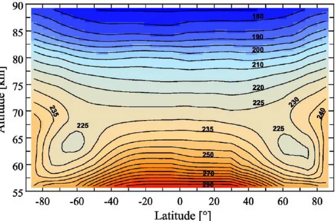
8 Two different regimes are recognizable (Fig. 3): below 70 km altitude, the temperature increases from the pole to the equator, above 70 km, the temperature increases poleward. At 80 km, a temperature of 205 K is found at the equator, 215 K at the poles (Limaye et al., 2018). Since the solar heating is higher at equator than poles, this trend indicates a significant role of atmospheric dynamics in the heat transfer above 70 km.

At the top of the mesosphere (70 – 90 km) the atmosphere is stressed by the thermal tides, day-to-night variations of heating caused by the incoming solar radiation (Limaye et al., 2018). Thermal tides are induced in the atmosphere by the solar cycle, and results from the combination of the rotation of Venus on its polar axis and of the revolution around the Sun. The diurnal cycle of the solar heating in the Venus atmosphere induces tides with wavenumbers 1 (diurnal), 2 (semi-diurnal), and higher orders.

Figure 3: Temperature structure of the mesosphere during nighttime. Cold collar features are clearly

recognizable around 60° - 70° (60 - 65 km altitude), at both hemispheres. Warmer regions are found around the poles. Haus et al., 2014, based on VIRTIS-M data.

(14)

9 The upper boundary of the mesosphere is the mesopause, which is located roughly between 95 and 120 Km. Temperature increases until ~ 103 km and then decreases until ∼ 110 km altitude. Although ozone has been detected on Venus (Montmessin et al. 2011) around 100 km, its abundance is too low to be responsible for this temperature inversion. No stratosphere has been observed on Venus between the troposphere and the mesosphere: the lack of a stable ozone layer, implies that this reversal of the temperature may be due to aerosols rather than ozone.

(iii) The thermosphere is the uppermost layer and it is more sensible to diurnal effects: while the dayside temperature is affected by the incoming solar radiation, the nightside is not provided with that heat and it is then – commonly – known as cryosphere: nighttime and daytime are separated by a sharp transition. On Venus the nighttime temperature in the thermosphere is very low, around 100 K, in contrast to 300 K on the dayside. These global oscillations of the atmosphere are forced by the thermal tides.

The average vertical temperature gradient in Venus’ dayside thermosphere is around 1.1-1.8 K/km (Muller-Wodarg et al., 2006), while it is negative during nighttime, reaching values of -1.2 K/km. Due to the lack of an internal magnetic field, the thermosphere is also the one interacting directly with the solar wind: this interaction produces the observed loss of oxygen ions (Luhmann et al., 2008) and neutrals compounds (Galli et al., 2008) and represents one of the mechanisms that produced the composition that we measure today. Besides the interaction with the solar wind, several other processes happen within the thermosphere: dissociation, ionization, thermal/nonthermal escape, cosmic ray erosion, meteoritic and cometary impacts.

1.3 Dynamics

To observe the atmospheric circulation, different methods have been adopted: these include Doppler Spectroscopy (Machado et al., 2017), direct observation through entry probes and balloons (Moroz and Zasova, 1997; Linkin et al, 1986), radio occultation techniques (Sànchez-Lavega, 2011), tracking of emission features (Drossart and Montmessin, 2015) and tracking of cloud features (Garate-Lopez et al., 2013).

(15)

10

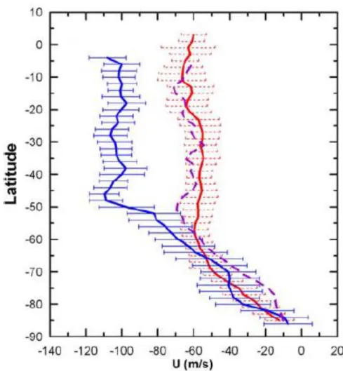
Figure 4: The averaged zonal wind speeds in the southern hemisphere of Venus as a function of latitude.

Retrieved by VIRTIS/VEX data. Blue lines are referred to 62-70 km altitude (top clouds), the purple lines to 58-64 km (base of upper clouds), the red lines to 44-48 km (lower clouds). Adapted from Sanchez-Lavega et al., 2008.

All probe data agree that the zonal wind speed from surface to 10 km altitude is less than 3 ms-1. From the surface to around 65–70 km, the zonal winds increase globally. Indeed, the mean atmospheric motions are dominated by a rotation that, at the cloud top level, is roughly 60 times faster than that of the planetary body: the upper atmosphere rotates in ∼4 days, the solid body in ∼243 days. The zonal winds blow westward, in the same direction of the planet rotation, with a nearly constant speed of ∼110 ms−1 (Garate-Lopez et al., 2013) at cloud top level (roughly 70 km altitude), from latitude 50° N to 50° S, then decrease their speeds monotonically from these latitudes toward the poles (Fig. 4). For that reason, Venus’ atmosphere is in a Retrograde Superrotation (RSR) state, or simply in “superrotation”.

(16)

11 The source of this superrotation and the mechanisms that maintain it, are still unknown. However, it is clear that large scale waves, in the form of planetary scale Kelvin waves and small-scale gravity waves (Sornig et al., 2008), play a major role in the efficient pumping of angular momentum through the atmosphere, from the inner layers to the outer ones. Studies (Newman and Leovy, 1992) suggest that the superrotation is maintained by the transport of retrograde zonal momentum upward through thermal tides at the equator and then poleward by the meridional cell. Indeed, in the upper cloud region, a major fraction of the solar energy incident is absorbed by the ‘unknown’ absorber and sulfuric acid aerosols. This distribution of the absorbed energy generates thermal tides, in the form of planetary-scale waves. The excited waves propagate both upwards and downwards from the forcing region.

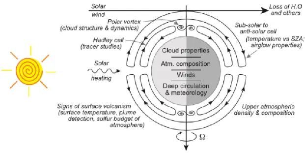
In addition to the zonal superrotation, a thermally directed meridional cell flowing from the equator to pole with meridional velocities of less than 10 ms−1 has been observed at the cloud top (Fig. 5). This meridional circulation is expected to be efficient in transporting warm air poleward and cooler air equatorward. Indeed, CO data obtained for the deep atmosphere by the NIMS onboard the Galileo spacecraft (Collard et al., 1993) and by Venus Express (Tsang et al., 2008), are consistent with a Hadley circulation on Venus that extends from the clouds to the surface, and from the equator to the poles. The less relevance that Coriolis forces have on Venus – with respect to

Figure 5: Schematic representation of the main Venus' circulation features. The main circulation is

superimposed to the subsolar to antisolar cell. Adapted by Piccialli, 2010 and Taylor and Grinspoon, 2009.

(17)

12 Earth – allows Hadley cells to extend much closer to the pole.

Above the clouds is present a transition region of complex dynamics that separates the Venus troposphere from the thermosphere: the winds decrease with altitude until a strong subsolar-antisolar (SS-AS) circulation occurs at 90-110 km, because of the large temperature gradient between Venus’ daytime and nighttime. By tracking emission features from NO and O2 airglow, we know that measurements in the 90–110 km altitude of the zonal component range from ∼ 5 to 150 ms−1, while wind data for the SS-AS range from 40 up to 290 ms−1, but exhibit very strong day to day variations. This SS-AS component seems to be related to the thermal tides: waves with both a diurnal and a semi-diurnal period have been observed through the data (Rossow et al., 1990; Collard et al., 1993), and a maximum has been detected in the temperature profile near the antisolar point, at around 90 km, corresponding to the adiabatic heating expected in the subsolar to antisolar circulation regime.

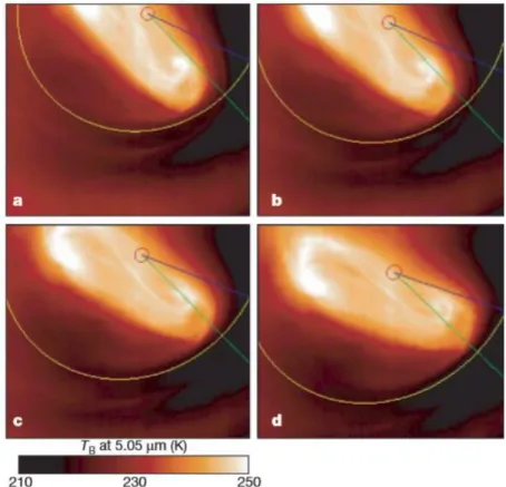
The complexity of the Venusian atmospheric dynamics finds its most puzzling element in the polar region (Fig. 6), where giant vortexes features are correlated to the subsidence of cold air and the consequent meridional flow due to the recycle of the air towards the equator. Vortexes occur in the polar region of planets: they are characterized by swirling clouds of high vorticity that move around a common center of rotation of low relative vorticity (the “eye”). The Venus’ polar vortexes appear like permanent – due to the lack of important seasonal variations – but time varying structures contained in a region ∼2500 km wide around the pole. Their position, rotation rate and morphology have been shown to change significantly: the basic core morphology is that of a single (monopole), double (dipole) or triple spiral, with filaments extending outwards from its center or connecting two or more brightness centers (Piccioni et al., 2007). Basing on cloud tracking measurements at 5.0 μm (∼65 km), Peralta et al. (2012) detected thermal tides harmonic forcing a solar-to-antisolar circulation across the pole, responsible of the dynamics of these vortex.

South-polar features observed in the atmosphere of Venus are in general similar to those observed around the north pole, with a slightly difference in the rotation period, maybe due to long terms variations in the dynamics, occurring between different observations: the Northern vortex exhibits a rotation period that spans from -2.79 to 3.21 days (Schofield and Diner, 1983; data from Pioneer Venus), while the Southern vortex shows a period of -2.48+- 0.05 days (Piccioni et al., 2007; data from Venus Express). Both rotate with an offset of a few degrees with respect to the geographical

(18)

13 pole.

The cold collar features circulate around the vortexes at latitudes between 60° and 80°, where the Hadley cells stop, dividing the middle atmosphere vertically and generating the two different regimes observed in the thermal structure of Venus: below, the atmosphere cools with increasing latitude, while above, it warms with increasing latitude (Kliore et al. 1985).

The dynamics behind the cold collar and the warm pole has only just begun to be investigated (Garate-Lopez et al. 2015). The presence of the cold collar between 55 and 65 km altitude appears to confine the warm vortex to latitudes poleward of 75°S, while at higher altitudes the vortex is more extended. Moreover, while warm poles need short-term processes or some with a certain periodicity (i.e. thermal tides), in order to maintain the pressure differences between the cold collar and the surroundings, some continually forcing mechanism is needed. In order to understand these features, as well as the general structure and dynamics of Venus atmosphere, coupling of observations and numerical models is needed.

Figure 6: Images at 5.05 μm, obtained by VIRTIS-M/VEX. The scale of

colors indicates the brightness temperature. The polar vortex is rotating around the geographical south pole (red circle) with an offset of 4°. The cold collar is just beyond the yellow line, which indicates the -70° parallel. Piccioni et al., 2007.

(19)

14

2. The Venus Express mission

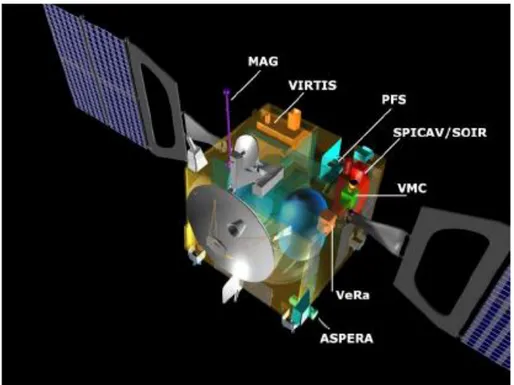
Venus Express was the first European mission to reach planet Venus (Titov et al., 2006; Svedhem et al., 2007). After a winning proposal in 2001, aiming to re-use much of the Mars Express basic design for the spacecraft, Venus Express was ready in less than 4 years. Launched by a Russian Soyuz-Fregat launcher on 9 November 2005, from Baikonur (Kazakhstan), it used a slightly modified spacecraft – with respect to Mars Express – in order to adapt to the specific environment around Venus, and a payload carrying the heritage of the Rosetta mission. Venus Express has been a quick-realization, cost-effective mission (Fig. 7).

Arrived at Venus on 11 April 2006, it entered a highly elliptic polar orbit of 24 h period, with a pericenter altitude of 250 km over the northern polar region and an apocenter altitude of 66,000 km over the southern polar region (Svedhem et al., 2009). This orbital geometry allowed a much dense coverage of the southern hemisphere with respect to the northern one.

Venus Express aimed at a complete investigation of the atmosphere and plasma environment of Venus and was also able to address some significant features of the surface. The quest of Venus Express can be summarized in seven key topics, according to Svedhem et al. (2007):

1) Atmospheric structure; 2) Atmospheric dynamics

3) Atmospheric composition and chemistry; 4) Cloud layer and hazes;

5) Energy balance and greenhouse effect; 6) Plasma environment and escape processes; 7) Surface properties and geology.

The payload was composed by seven scientific instruments, devoted to answer to the topics above. We provide here a brief overview of the general characteristics (Table

1) and objectives of the instruments onboard Venus Express mission. A more detailed

description of VIRTIS and VeRa experiments – on which data this work is based – will be given in section 2.1 and section 2.2, respectively.

(20)

15

SPICAV/SOIR (Spectroscopy for the Investigation of the Characteristics of the

Atmosphere of Venus/Solar Occultation in the Infrared) (Bertaux et al., 2007) was a set of three UV-IR spectrometers (SPICAVUV, SPICAV-IR, SOIR) to study the thermal profiles and composition of the Venus thermosphere (90-140 km), as well as vertical profiles of the haze above the clouds and the microphysical properties of aerosols within the haze, by means of solar and stellar occultations.

VMC (Venus Monitoring Camera) was a wide-angle camera working in four

narrows spectral bands (Markiewicz et al., 2007). The visible band studied water vapor absorption and O2 airglow emission; the UV band tracked the clouds top in reflected sunlight during daytime, thanks to the unknown UV absorber; the two near-IR bands mapped the global distribution of water vapor and the surface brightness during nighttime.

PFS (Planetary Fourier Spectrometer) was a high spectral resolution

IR-spectrometer with two channels (Formisano et al., 2006). Its purposes were to map the temperature field in the 55–100 km altitude range and on the surface, along with a determination of the total radiation budget and the extraction of the abundances profile in the middle and lower atmosphere. However, the mechanism that had to point the field of view of the Spectrometer towards Venus did not move properly after launch.

ASPERA-4 (Analyzer of Space Plasma and Energetic Atoms) included five

sensors: two Neutral Particle Detectors (NPD1 and NPD2), a Neutral Particles Imager (NPI), an Electron Spectrometer (ELS) and an Ion Mass Analyser (IMA) (Barabash et al., 2007). ASPERA-4 made measurements in the solar wind and characterized the outer atmospheric regions with respect to flux, energy and composition of the particles (i.e. the determination of the escape rates of H+, O+ and He+).

MAG (Magnetometer) was a dual sensor fluxgate instrument devoted to measure

magnitude and direction of the magnetic field around Venus (Zhang et al., 2006). MAG, devoted to the study of the plasma environment of Venus, produced continuous measurements, studying the bow shock and the induced magnetopause.

VIRTIS (Visible and Infrared Thermal Imaging Spectrometer), is described in section 2.1.

(21)

16

Figure 7: Schematic representation of Venus Express spacecraft. Locations of the instruments are displayed. Copyright by ESA.

2.1 The Visible and Infrared Thermal Imaging Spectrometer

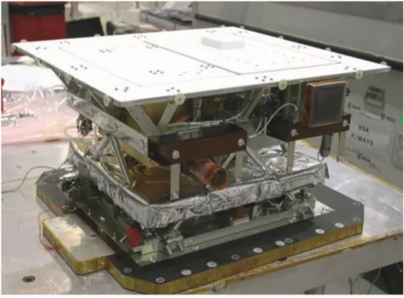
VIRTIS, the Visible and Infrared Thermal Imaging Spectrometer (Fig. 8), used a concept and a design very similar to the VIRTIS instrument that flew on the Rosetta spacecraft (Coradini et al., 1998), with some modifications to adapt it to the different environment and target brightness.

VIRTIS was divided in four modules: the Optics Module containing the Optical Heads, the two Proximity Electronics Modules and the Main Electronics Module. Two subsystems were located into the Optics Module: VIRTIS-M, a visible and infrared (0.3 μm up to 5.1 μm) spectro-imager, and VIRTIS-H, an infrared (2 μm up to 5 μm) point spectrometer, which was aligned with the center of the VIRTIS-M field of view (Piccioni et al., 2007; Drossart et al., 2007).

The two optical systems of VIRTIS had parallel slits and were placed at the top of the Optics Module, which was directly coupled to the radiator and the space. The infrared sensors were actively cooled to 80 K, while the visible detector was passively cooled below 200 K.

(22)

17

Table 1

Name General characteristics

SPICAV/SOIR Wavelengths: 110–310 nm; 0.7-1.7 µm; 2.2-4.4 µm.

Resolving power up to λ/Δ λ >20000.

VMC Wavelengths: 365 nm, 513 nm, 965 nm, and 1000 nm.

FOV: 17.5°, pixel size on the surface: 200 m (pericenter) - 45 km (apocenter).

PFS Wavelengths of the two channels: 0.9–5.5 µm and 5.5–45 µm. Spectral resolution: 1.3 cm-1.

ASPERA-4 Neutral particles energies: 0.1-60keV;

Electrons energies: 1eV-15keV; ions energies: 0.01-36keV/q

MAG Frequency of solar wind samples: 1 Hz.

Frequency of pericenter samples: up to 128 Hz.

VIRTIS VIRTIS-M spectral range: 0.3-5.1 µm;

VIRTIS-M spectral sampling: 2 nm (VIS) – 10 nm (IR). VIRTIS-H spectral range: 2-5 µm;

VIRTIS-H spectral sampling: 1.5 nm.

VeRa Wavelength of the “X band”: 3.6 cm.

Wavelength of the “S band”: 13 cm.

VIRTIS-M had a field of view of 64 x 64 mrad, correspondent to a pixel size of 0.25 mrad. It was divided in two spectral channels: the Visible channel (VIS) covered the spectral range 0.3-1.1 μm, with a spectral sampling of about 2 nm, the Infrared channel (IR) covered the spectral range 1.05-5.1 μm, with a spectral sampling of about 10 nm. VIRTIS-M was able to acquire simultaneously the spectra of a slit of aligned pixels. Acquisitions with different pointings allowed to produce a monochromatic two-dimensional image of the target (a “cube”), which contained spectral information for each pixel. VIRTIS-M produced cubes having typically a spatial dimension of 256 x 256 (samples x lines) and a spectral dimension of 432 different wavelengths (bands), covering the entire probed spectral range.

VIRTIS-H had a field of view of 0.44 x 1.34 mrad, which means a projected horizontal resolution per pixel of 115 km × 38 km at the apocenter. Its spectral sampling

(23)

18 was about 1.5 nm, finer than VIRTIS-M. VIRTIS-H provided spectra (sampled in 432 wavelengths) in the center of VIRTIS-M images.

VIRTIS dataset is made of several acquisitions, for each orbit around Venus, spanning over more than 3000 operational days. Cubes of geometry are associated with every observation: they contain geometrical information of the target, as longitude, latitude, height with respect to the surface, incidence angle, emission angle etc.

Figure 8: VIRTIS Optics Module. VIRTIS-M and VIRTIS-H are just under the cover (right and left of the image, respectively).

VIRTIS experiment studied the atmosphere composition, leading to accurate measurements of chemical species abundances (Marcq et al., 2008). It investigated the atmospheric dynamics, measuring the wind speeds by tracking the clouds in the UV (top clouds, ~70 km altitude on dayside) and IR (bottom clouds, ~50 km altitude on nightside) and following the time variation of dynamical-tracking species (e.i., CO, OCS) (Marcq et al., 2008). It mapped the surface of Venus in the 1 μm spectral window during nighttime and searched for volcanic and seismic activity (Mueller et al., 2008).

(24)

19 Moreover, radiance spectral distribution contains information about temperature distribution. Since opacity varies with wavelength and the depth from which emergent radiation is emitted varies with opacity, different depths within the atmosphere are sounded by measurements at different wavelengths. Radiation emitted from gases of known distribution, such as carbon dioxide, allows the retrieval of temperature. For this reason, VIRTIS dataset was extensively used to probe the mesosphere temperature structure of Venus (Grassi et al., 2014; Migliorini et al., 2012).

2.1.1 VIRTIS-M temperature retrieval and database selection

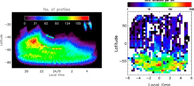
VIRTIS-M temperature retrieval by Grassi et al. (2014) is based on Bayesian formalism (Rodgers, 2000). The temperatures have been retrieved from the CO2 band at 4.3 μm. The presence of CO2 non-Local Thermal Equilibrium emission and the atmospheric scattering of the sunlight presently limit this study to nighttime only. Constrains, imposed in order to avoid signal saturation of data due to the thermal emission of the instrument, select a dataset of 636 VIRTIS-M cubes, acquired until August 2008. The coverage of this dataset is in general more dense in the southern hemisphere, from mid latitudes to the pole (Fig. 9).

In this work, we used the entire dataset of Grassi et al. (2014).

Figure 9: Spatial coverage of the VIRTIS-M dataset adopted for the temperature retrieval (left panel, Grassi et al., 2010). Spatial coverage of the VIRTIS-H dataset adopted for the temperature retrieval (right panel, Migliorini et al., 2012).

(25)

20 2.1.2 VIRTIS-H temperature retrieval and database selection

VIRTIS-H temperature retrieval by Migliorini et al. (2012) relies on a methodology similar to Grassi et al. (2014). This study is limited to 3 × 104 VIRTIS-H spectra collected until November 2013. VIRTIS-H complements the dataset of VIRTIS-M with more observations at low latitude and in the northern hemisphere, even if the larger part of valid retrievals is still in the mid to high latitude range of the southern hemisphere (Fig. 9).

In this work, we used the entire dataset of Migliorini et al. (2012).

2.2 Venus Express Radio Science Experiment

VeRa, the Venus Express Radio Science Experiment, used radio signals in two

different bands “X” and “S” (3.6 and 13 cm respectively) to study the Venus atmosphere and ionosphere.

VeRa studied:

(1) the atmospheric structure (approximately 40 km to 90 km altitude), basing on vertical profiles of neutral mass density, temperature, and pressure as a function of local time and season;

(2) the presence and properties of small scale and planetary waves, indicating that convection at low latitudes and topographical forcing at high northern latitudes play key roles in the genesis of gravity waves and demonstrating the role of thermal tides in the mesosphere;

(3) the H2SO4 vapor layer in the atmosphere by variations in signal intensity; (4) the ionospheric structure from approximately 80 km to the ionopause (600 km), allowing investigation of the solar wind plasma.

2.2.1 VeRa temperature profiles extraction and database selection

Measurements have been made by directing the High Gain Antenna (HGA) towards the Earth before and after occultation of the spacecraft behind the planetary disc of Venus. The atmosphere caused the radio path to bend: the propagation of the radio signal through the ionosphere and the neutral atmosphere of Venus led to a change in the radio ray path, that produced a wave’s phase shift detectable as a frequency shift on Earth. This allowed retrieval of electron density profiles in the ionosphere and profiles of temperature, pressure and neutral number density in the mesosphere and upper troposphere with a high vertical resolution. The radio occultation technique

(26)

21 allows to sound deeper below the clouds, probing altitudes deeper than VIRTIS could reach.

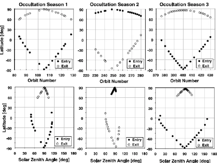
Due to the orbit geometry of Venus Express, VeRa coverage of the Northern hemisphere is poor too. Indeed, while the southern hemisphere could be observed with good latitudinal coverage during each occultation season, observations in the northern hemisphere are mainly constrained to latitudes close to the pole (Fig. 10).

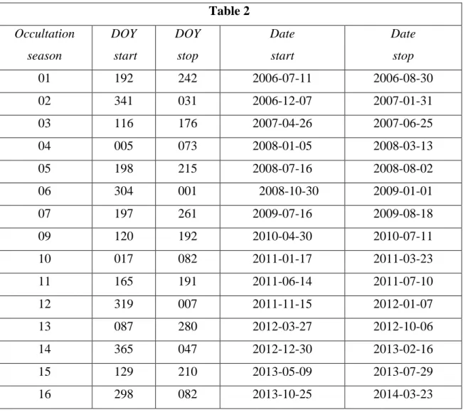
The VeRa database (Table 2) contains a collection of the atmospheric temperature, pressure, absorptivity, sulfuric acid vapor (H2SO4) and ionospheric electron density profiles, from each of the VeRa occultation season, along with the latitudinal and local time averaged atmospheric temperature and the corresponding pressure profiles.

In the present study, we selected all nighttime observations form the entire database (local time between 18:00 and 6:00). At the end of the selection phase, we found 657 VeRa profiles corresponding to our requirements, acquired up to November 2013. We used these profiles to perform our study.

Table 2 Occultation season DOY start DOY stop Date start Date stop 01 192 242 2006-07-11 2006-08-30 02 341 031 2006-12-07 2007-01-31 03 116 176 2007-04-26 2007-06-25 04 005 073 2008-01-05 2008-03-13 05 198 215 2008-07-16 2008-08-02 06 304 001 2008-10-30 2009-01-01 07 197 261 2009-07-16 2009-08-18 09 120 192 2010-04-30 2010-07-11 10 017 082 2011-01-17 2011-03-23 11 165 191 2011-06-14 2011-07-10 12 319 007 2011-11-15 2012-01-07 13 087 280 2012-03-27 2012-10-06 14 365 047 2012-12-30 2013-02-16 15 129 210 2013-05-09 2013-07-29 16 298 082 2013-10-25 2014-03-23

(27)

22

Figure 10: Latitudinal coverage of VeRa season 1, season 2 and season 3 occultations. Full circles: ingress. Empty circles: egress. Tellmann et al. (2009).

(28)

23

3. General Circulation Models

The link between the data gathered by remote sensing measurements and the interpretation of the physical processes active in planetary atmospheres, is made by numerical models: they are valuable instruments to understand the most peculiar features in the atmospheres of planets and the mechanisms behind their dynamics and evolution. Given proper parameters (i.e. radius, gravity, rotation period), boundary conditions, damping and forcing mechanisms, these simulations reproduce the large-scale circulation of a planet, solving the equations governing the atmospheric dynamics. These numerical models are called General Circulation Models (GCMs).

In the attempt of building numerical simulations able to reproduce or predict the available observations of a given planetary body, GCMs combine:

(1) a three-dimensional hydrodynamical core to solve the Navier-Stokes equations for a rotating spherical system (three components of the momentum equation, the continuity equation for density, the thermodynamic equation for potential temperature, the equation of state and the transport equations for tracers);

(2) a radiative transfer solver;

(3) a parameterization of turbulence and convection not resolved by the dynamical core;

(4) a thermal ground model, considering storage and conduction of heat; (5) a volatile phase change code for the surface or the atmosphere.

Most of the GCMs adopted in planetary science are a re-adaptation of their counterparts for Earth atmosphere. They have been used for the study of several bodies of the Solar System, such as Mars (Forget et al., 1998), Saturn (Spiga et al., 2013), Pluto (Forget et al., 2017), Titan (Lebonnois et al., 2012) and Triton (Vangvichith et al., 2010) and also for conducting scientific investigations on the possible climates of exosolar planets (Turbet et al., 2016).

The planet Venus makes no exception and it has been widely studied thanks to GCMs. However, the extreme physical conditions of its atmosphere and the very important role of the clouds in the energy balance of the planet, impose a much difficult

(29)

24 work of adaptation. Producing a GCM for Venus is a big challenge to be accomplished, because of the sensitivity showed by the dynamical core to the initial conditions and the weak forcing of Venus atmosphere (Bengtsson et al., 2013). For this reason, it is difficult to draw conclusions on the circulation obtained with a single model and the capability of that model to conserve the angular momentum, as well as on its sensitivity to many parameters.

In the modelling of Venus, two different approaches have been used through the years:

i) A simplified approach. The radiation scheme is not based on a radiative transfer model; it uses a linear temperature relaxation scheme towards a global-averaged temperature profile obtained from data, plus a perturbations function that takes into account the latitudinal variations of solar radiation within the cloud deck. The circulation is characterized through simplified heating, cooling and friction processes, as well as a rough representation of surface and clouds.

ii) A physically-based approach. It relies on a radiative transfer module that computes the temperature structure self-consistently for each different atmospheric layer. It makes use of realistic topography and specific heat as well. The simulation requires longer computational times, but the outputs point directly toward the physical processes. The aim is not only a qualitative description of the atmosphere of Venus, but a general and comprehensive view of all the active mechanisms.

Either using a simplified or a physically-based approach, some key scientific questions are typically investigated by GCMs and need to be answered in order to understand the real nature of the circulation of Venus:

1. What are the mechanisms that produce fast zonal winds from a slow rotating body? 2. What is the role of the waves, in particular gravity waves and thermal tides;

3. How much is important the topography in surface-atmosphere interactions and in building up superrotation?

(30)

25 5. What is the origin of the polar temperature distribution, formed by highly variable

vortices and cold air areas (the cold collar)?

6. What kind of mechanism permanently forces the cold collar?

At the present state, several simulations qualitatively reproduced the observed superrotation in the modelled atmospheres. However, their results vary from case to case, showing different zonal wind fields under similar initial conditions.

GCMs have also been able to demonstrate the role of the thermal tides in the vertical transportation of angular momentum through the atmosphere, as well as the role of planetary-scale waves and large-scale gravity waves.

However, the thermal structure is still a pending issue in the modelling of Venus. In particular, the polar temperature distribution has not been satisfactory reproduced.

3.1 Simplified Venus General Circulation Models

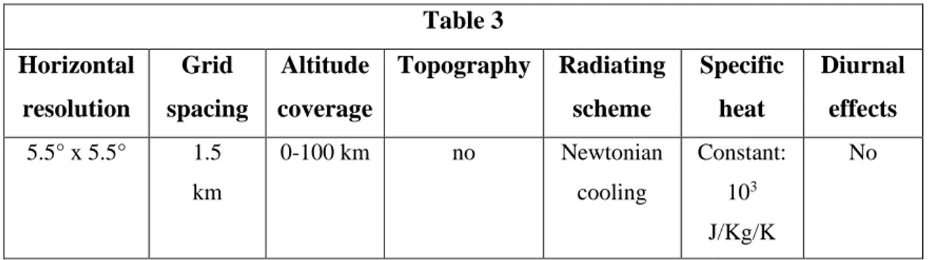
3.1.1 The CCSR/NIES model

Table 3 Horizontal resolution Grid spacing Altitude coverage Topography Radiating scheme Specific heat Diurnal effects 5.5° x 5.5° 1.5 km 0-100 km no Newtonian cooling Constant: 103 J/Kg/K No

The CCSR/NIES model (Center for Climate System Research/National Institute for Environmental Study) (Table 3, Fig. 11) is born as an adaptation of a spectral model used for terrestrial modelling (Yamamoto and Takahashi, 2003). A simplified radiative process of zonally uniform solar heating has been assumed and temperatures are relaxed via Newtonian cooling. Solar heating due to CO2 above 70 km and surface radiative

processes are neglected.

The altitude of the maximum heating rate has been adapted to peak 10 km below the cloud top, in order to fully develop a superrotation with 100 m/s at cloud top. No superrotation is activated when the heating rate peaks at cloud top, like in the observations. The circulation is formed by two Hadley cells.

(31)

26

In Yamamoto and Takahashi (2004) and Yamamoto and Takahashi (2006), a new three-dimensional solar heating and Newtonian cooling has been implemented. The peak of the solar heating is located at altitude closer to data, but the heating rate at 55 km has become higher than observations. An equatorial Kelvin wave, a midlatitude Rossby wave – transporting angular momentum towards the equator – and thermally-induced, global scale waves are developed within the model.

Including aerosols, CO2 and H2O absorption and emission (Ikeda et al., 2007), the

vertical temperature structure below 70 km is found to better agree with observations. Superrotation is maintained by the coupling of the mean meridional circulation with thermal tides, but appear fully developed just above 55 km. Under 55 km, the zonal wind is weaker: only introducing a parametrization for gravity waves, superrotation becomes fully activated.

Figure 11: Altitude-latitude distribution of the longitudinally averaged zonal winds (m/s, left panel) and temperatures (K, right panel). Yamamoto and Takahashi (2012).

In Yamamoto and Takahashi (2012, 2015), after inducing superrotation through wave forcing, a Y-shaped wave pattern is formed in the cloud by the superposition of equatorial Kelvin waves and midlatitude Rossby waves, and seems to be modulated by thermal tides. At the same time, an unstable polar vortex is simulated, its life strongly affected by the transient waves: this vortex is sometimes modeled as a dipolar feature, sometimes merges into a monopole or breaks up into a tripole as it stretches. In general, when the transient waves are in phase within the hot oval, the dipole is enhanced, otherwise, the dipolar structure breaks down. The results show some discrepancies with

(32)

27 observations: the cold collar is not adequately reproduced, as well as the fine structures observed in the pole, because of the low horizontal resolution utilized in the runs.

3.1.2 The OPUS-V model

Table 4 Horizontal resolution Grid spacing Altitude coverage Topography Radiating scheme Specific heat Diurnal effects 5° x 5° 3.5 km 0-90 km flat Newtonian cooling / radiation scheme Constant: 103_J/Kg/K no

The OPUS-V (Oxford Planetary Unified Simulation model for Venus) (Table 4,

Fig. 12) was developed in Oxford (Lee et al., 2005), using a modification of the UK Meteorological Office Hadley Center Atmospheric Model (HadAM3). It is a finite-difference model, implemented with a simple bulk cloud parametrization (Lee and Richardson, 2010). The radiation scheme is obtained by a relaxation towards Pioneer Venus temperature profile, plus a function that compute the latitudinal variability of the solar absorption rate in the cloud deck (Seiff et al., 1980).

In each hemisphere, zonal jets are produced at 60 km, with a maximum of 45 m/s at mid-latitudes, and an equatorial wind of 35 m/s: this discrepancy with observations may be related to the coarse horizontal resolution, unable to reproduce sub-gridscale convection. Due to the slower zonal winds, both Kelvin waves and Rossby waves in the model display a period longer than in observations. Mid-to-high latitudes cold regions and warm poles are reproduced, at 6 x 104 Pa and 7 x 103 Pa, respectively, but the contrast with the surroundings is smaller than data; moreover, the fine structure observed in these features does not appear in the GCM.

In Lee et al. (2010) a cloud parameterization has been added, including a close cycle of condensation, evaporation and sedimentation of sulfuric acid particles, where the surface acts as a reservoir for the sulfuric acid liquid. Large "Y"-shape clouds are modeled, similar to those observed. These clouds maintain their large-scale structure over a period of about 7 days, and then become "C"-shape features, due to the

(33)

28 interaction of polar and equatorial waves, the former having a longer period than the latter.

Figure 12: Left panel: pressure-latitude distribution of the longitudinally averaged zonal winds (m/s, Lee et al., 2007). Right panel: polar temperatures at 6 x 104_{Pa (K, Lee et al., 2005).}

Implementing a more realistic radiation scheme to include cloud scattering, Mendonca (2010) and Mendonca et al. (2012), reproduce a long-term variability of the zonal winds in the cloud region, related to large-scale variations in the atmospheric circulation of the low atmosphere. The simulated circulation is characterized in the cloud region by two planetary-scale Hadley cells in each hemisphere, one near the cloud base and another in the upper clouds. The model is still unable to reproduce the strong zonal winds retrieved by data, especially in the lower atmosphere. Even utilizing a realistic topography seems inefficient in building up superrotation.

3.1.3 The AFES model

Table 5 Horizontal resolution Grid spacing Altitude coverage Topography Radiating scheme Specific heat Diurnal effects 2.8° x 2.8° 1.5 km 0-120 km no Newtonian cooling Constant: 103 J/Kg/K No/yes

(34)

29 The AFES model (Atmospheric GCM for the Earth Simulator) (Table 5, Fig. 13) is a spectral model (Ando et al., 2016) developed in several horizontal and vertical resolution, that uses solar heating rates based on observations by Tomasko et al. (1980).

The simulation was ran with and without solar heating variation: without diurnal effects, the modelled zonal wind fields and temperature profiles are not in agreement with data, vice versa, introducing diurnal variation in the solar heating, model and data become much in agreement, giving a hint of the importance of the thermal tides in the atmospheric circulation of Venus. Superrotation is activated since the first kilometers, with zonal winds showing a mid-latitude peak of 120 m/s at 103 Pa, and a strong polar vertical shear which redistribute the angular momentum downward.

Figure 13: Altitude-latitude (northern hemisphere) distribution of the zonally and temporally averaged zonal winds (m/s, left panel) and temperatures (K, right panel). Ando et al. (2016).

The modelled temperature rises towards the pole at 75 Km and decreases monotonically in the same direction at 60 Km, as observations have revealed. A cold region appears (20 K colder than the surroundings), resembling the cold collar; it is located between 60° and 70°, at an altitude slightly higher than data (Ando et al., 2016). A vortex, rapidly changing in shape, rotates around the pole with an offset of a few degrees.

Also the capability of the GCM to reproduce the warm pole variability and the thermal inversion resembling the cold collar, is directly linked to the presence of a

(35)

30 diurnal component in the solar heating. It is shown that the diurnal component causes the model to have a strong downward motion in the polar region, which is responsible of the efficient adiabatic heating that produces the warm pole. When the diurnal component is not activated, the adiabatic heating is less effective, and both the cold region and the warm pole disappear. The role of thermal tides in the GCM is deeply investigated in Takagi et al. (2018), where it was showed that the peak amplitudes of the vertical winds induced by thermal tides are important until higher harmonics: 3rd and 4th thermal tides subharmonics in the AFES-Venus GCM simulations are roughly 50% and 25%, respectively, compared to the 2nd component.

3.2 Physically based Venus General Circulation Models Table 6 Horizontal resolution Grid spacin g Altitude coverag e Topograph y Radiatin g scheme Specific Heat Diurna l effects 3.75°x1.875° 2 km 0-90 km Magellan Full transfer module Analytical approximatio n yes

The dynamical core of the IPSL (Institut Pierre Simon Laplace) Venus GCM (Table 6, Fig. 14, Fig. 15) is based on the Earth model developed at the Laboratoire de Météorologie Dynamique of Paris, which is a latitude-longitude grid finite-difference dynamical core. The model has the capability to zoom over a given region.

Crespin et al. (2006) presented the initial results for a simulation aiming to produce a realistic Venus GCM. In Lebonnois et al. (2010) the GCM included a realistic topography taken from Magellan mission, a realistic diurnal cycle, a temperature dependence of the specific heat Cp(T), in order to get realistic adiabatic lapse rates in the entire atmosphere, and a radiative transfer module which allowed a consistent computation of the temperature field. The boundary layer scheme was taken by Mellor and Yamada (1982).

With these ingredients, peak speeds of 60 m/s are activated at cloud top. Without introducing a realistic topography, superrotation is not activated by the model.

The impact of diurnal cycles has been highlighted by the IPSL Venus GCM. Without diurnal variation, the angular momentum transport is consistent with other

(36)

31

GCMs, with clear high and mid-latitude jets in the winds field. Introducing a diurnal variation, the thermal tides add a significant downward transport at the equator, that weakens the upward and poleward transport due to the mean meridional circulation. This transport allows accumulation of angular momentum at low latitudes and prevents the formation of mid and high-latitude jets.

Lebonnois et al. (2016) improved the modelling capabilities of the IPSL Venus GCM. A fully developed superrotation is obtained, both from rest and from an atmosphere already in motion, though winds below the clouds are about half the observed values. The atmospheric waves play a crucial role in transporting angular momentum in Venus atmosphere, with diurnal and semidiurnal tides dominating in the upper clouds level. This work was also capable to successfully reproduce the cold feature displayed in Ando et al. (2016) around 60°-70° latitude, but having just a 10 K contrast with the surroundings. As it happens in Ando et al. (2016), this cold collar resembling feature is formed at an altitude higher than data.

Figure 14: Pressure-latitude distribution of the mean zonal wind field (m/s). Lebonnois et al.

(37)

32

Garate-Lopez and Lebonnois (2018) introduced a latitudinal variability in the parametrization of the clouds, taken by Haus et al. (2014, 2015). This cloud model prescribes the vertical distribution for the three cloud particle modes observed in Venus clouds. It includes a latitudinal modulation of these distributions: a strong decrease of the cloud top altitude is present at 50° latitude, dropping from 70 km to 61 km over both poles, along with a latitudinally dependent scaling of the abundance of the different modes compared to the equatorial vertical distributions.

Solar heating rates are computed from tables that give the heating rates as a function of altitude, solar zenith angle, and latitude. This cloud model is also added in the infrared net exchange matrices. In order to implement the latitudinal variation of the cloud structure in the infrared cooling rates, the net-exchange rate matrices are computed for five latitudinal bins and then interpolated between the central latitudes of each bin. These matrices use correlated-k coefficients of opacity sources, gas and clouds, and consider the CO2 and H2O collision-induced absorption.

Because of the uncertainty of the optical properties and the absorption of the solar flux, due to the lack of knowledge of the lower-haze particles composition, some tuning in the radiative transfer module were possible, in order to bring the modelled temperature profile in much agreement with the observed values: as the simulated temperature structure in the deep atmosphere was colder (10 K) than that observed, the solar heating rates were increased in the 30–48 km altitude region by multiplying the values provided by Haus et al. (2015) of a factor of 3. Moreover, some additional continuum to close the infrared windows located in the 3–7 μm range was also needed below the clouds (16 to 48 km), in order to have a best fit of the VIRA and VeGa-2 temperature profiles.

Garate-Lopez and Lebonnois (2018) show that the cloud structure is essential in polar temperature structure and dynamics. The cold region appearing at mid-to-high latitude in Ando et al. (2016) and Lebonnois et al. (2016) weakens, although still present. Even more striking, for the first time a cold collar feature is reproduced at the right altitude (2 x 104 Pa – 4 x 103 Pa) and latitude (poleward of 60°), with a realistic contrast against the surroundings.

(38)

33

Figure 15: Zonally (360°) and temporally (2 Venus days) averaged temperature field (K). Garate-Lopez and Lebonnois (2018).

At the present state, the simulation in Garate-Lopez and Lebonnois (2018) is the state of the art IPSL Venus GCM, the version that we used in the comparison presented in this work. More details about this simulation and the main characteristics of the radiative transfer scheme, can be found in Garate-Lopez and Lebonnois (2018). An accurate description of the general characteristics of the IPSL Venus GCM and the dynamical core is given in Lebonnois et al. (2010).

(39)

34

4. Data-model comparison: thermal and winds field

Here we present the validation of the current version of the IPSL (Institut Pierre Simon Laplace) Venus GCM, by means of a comparison between the modelled temperatures and winds field and those obtained from data by the Visible and Infrared Thermal Imaging Spectrometer (VIRTIS) and the Venus Express Radio Science Experiment (VeRa) onboard Venus Express.

As already stated in chapter 2, in this work we made use of the entire dataset from Grassi et al. (2014) and Migliorini et al. (2012), respectively providing VIRTIS-M and VIRTIS-H temperature retrieval, as well as all nighttime observations form the entire VeRa database (local time between 18:00 and 6:00). The IPSL Venus GCM temperatures and winds are based on the latest version of the model, as obtained by Garate-Lopez and Lebonnois (2018) simulation (see chapter 3). While the modelled and observational temperature fields comparison relies on the original data analysis conducted in the present work, starting from Grassi et al. (2014) and Migliorini et al. (2012) temperature retrieval, the wind fields comparison directly uses the data analysis by Sanchez-Lavega et al. (2008), based on VIRTIS data cloud tracking.

In order to validate the global thermal and winds field characterization of the Venus atmosphere obtained with the IPSL Venus GCM, we first analyze the zonally and temporally averaged temperatures and winds field, that are easy to compare with Venus Express observations and give an immediate idea of the overall model reliability.

We limit our analysis to the southern hemisphere, which is richer in observational data. Indeed, we would expect Venus to be a symmetric planet (little axis inclination, no seasonal variations, no macroscopic topographic asymmetries between hemispheres, except for the Maxwell Montes) and we can extend any consideration done for the southern hemisphere to its northern counterpart. Also, because the model itself would eventually show us any possible asymmetry of the planet: the two hemispheres are almost identical in the IPSL Venus GCM. Therefore, from here on, we just report the discussion for the – better observationally covered – southern part of the globe.

The adopted datasets, along with a general description of the VIRTIS and VeRa experiments and the methods of acquisition and retrieval, have been described in section

2.1 and section 2.2. In section 4.1 we will focus on the thermal field, while in section 4.2