The central Italy seismic sequence between August and
December 2016: analysis of strong-motion observations
Luzi L.1, Pacor F.1, Puglia R.1, Lanzano G.1, Felicetta C.1, D’Amico M.1, Michelini A.1,
Faenza L.1, Lauciani V.1, Iervolino I.2, Baltzopoulos G.3, Chioccarelli E.3
Corresponding author: Lucia Luzi, Istituto Nazionale di Geofisica e Vulcanologia, via Corti 12, 20133 Milan (Italy), [email protected]
1 Istituto Nazionale di Geofisica e Vulcanologia (INGV), Italy
2 Dipartimento di Strutture per l’Ingegneria e l’Architettura, Università degli Studi di Napoli
Federico II, Italy
3 Istituto per le Tecnologie della Costruzione - Consiglio Nazionale delle Ricerche
(ITC-CNR), URT at Dipartimento di Strutture per l’Ingegneria e l’Architettura, Università degli Studi di Napoli Federico II, Italy
Abstract
Since August 2016, central Italy has been struck by one of the most important seismic sequences ever recorded in the country. In this study, a strong-motion data-set, consisting of nearly 10,000 waveforms has been analysed to gather insights about the main features of ground-motion, in terms of regional variability, shaking intensity and near-source effects. In
particular, the shakemaps from the three main events in the sequence have been calculated, in order to evaluate the distribution of shaking at a regional scale, and a residual analysis has been performed, aimed at interpreting the strong-motion parameters as functions of source distance, azimuth and local site conditions. Particular attention was dedicated to near-source effects (i.e., hanging/foot wall, forward-directivity or fling-step effects). Finally, ground-motion intensities in the near-source area have been discussed with respect to values used for structural design.
In general, the areas of maximum shaking appear to reflect, primarily, rupture complexity on the finite faults. Large ground motion variability is observed along the Apennine direction (NW-SE), that can be attributed to source-directivity effects, especially evident in the case of small-magnitude aftershocks. Amplifications are observed in correspondence to
intra-mountain basins, fluvial valleys and the loose deposits along the Adriatic coast. Near-source ground motions exhibit hanging wall effects, forward-directivity pulses and permanent displacement.
1. Introduction
Since August 2016, an extended region of central Italy has experienced a long lasting seismic sequence [still active at the time of submission of this work]. Until December 2016, three main events with magnitude larger than 5.5 (Figure 1) struck an area approximately more than 50 km long and 30 km wide. The initiating event was the Amatrice earthquake (Mw 6.0) that occurred on August 24, 2016 at 1:36:32 UTC and strongly damaged the villages
of Amatrice and Accumoli. Despite the fact that the population exposed to VIII+ Mercalli Cancani Sieberg (MCS) intensity was relatively small (7,500 to 10,000 inhabitants), the
earthquake caused about 300 fatalities, resulting from the collapse of several buildings in the towns and villages closest to the epicentre. A second event (Mw 5.9), occurred farther north,
on October 26, 2016 at 19:18:06 UTC, near the village of Ussita (Figure 1), resulting in additional damage to the buildings and main infrastructures previously hit by the August 24 event. The third and largest event (Mw 6.5), occurred on October 30 2016 at 06:40:18 UTC
with the epicenter located close to Norcia (Figure 1). It caused the total collapse of several structures damaged by the previous events and the complete destruction of the village of Amatrice. Fortunately, there were no fatalities caused by the October events, as most of the population had been evacuated already. These seismic events triggered extended secondary effects like ground failures (widespread surface faulting, ground cracks and landslides) and deep-seated landslides as described by Pucci et al (2017) and Huang et al (2017).
The area affected by the sequence is located in the central Apennine belt in Italy, a region characterized by crustal extension, where NNW-SSE and NW-SE striking normal and normal-oblique faults, active since the early Quaternary, are superimposed to a pre-existing strike-slip and fold-and-thrust belt structure (Lavecchia et al., 1994; Lavecchia et al., 2002; Calamita and Pizzi, 1994; Cello et al., 1997; Vezzani et al., 2010). The fault segments generally dip south-westwards, extending 20–25 km along-strike and 10–15 km along-dip (Boncio et al., 2004). Their typical en echelon pattern locally originates intra-mountain basins, such as the Norcia plain (Galadini and Galli, 2000; Boncio and Lavecchia, 2000).
Moderate and strong seismic events struck this area in the past decades (Gubbio 1984, Mw
5.6; Colfiorito 1997, Mw 6.0; Norcia 1979, Mw 5.9; L’Aquila 2009, Mw 6.1; see Figure 1). All
these earthquakes featured focal mechanisms consistent within the regional NE–SW tensional stress field.
The three main shocks of the central Italy sequence occurred along a fault alignment that extends from Mt. Vettore - Mt. Bove to Mt. Gorzano (VBF and GF, respectively, in Figure 2), lies to the east of the alignment that develops from Gubbio to Colfiorito and extends as far as to the area struck by the 2009 L’Aquila sequence to the south (Figure 1).
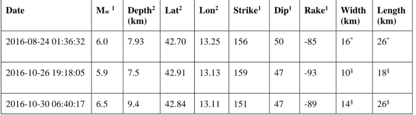
The causative fault mechanism of the three main shocks herein considered, obtained from Time Domain Moment Tensor (TDMT) technique (Dreger and Helmberger, 1993) and implemented at Istituto Nazionale di Geofisica e Vulcanologia (INGV) National Earthquake Centre (Scognamiglio et al, 2010), features pure normal faulting, in agreement with the prevailing extensional regime of the central Apennines and with the mechanisms of the Colfiorito and L’Aquila earthquakes (Scognamiglio et al., 2016). The characteristics of these events are reported in Table 1.
The aim of this work is to provide: (i) a description of the ground motion associated with the sequence between August and December 2016 through the comparison with Ground Motion Prediction Equations (GMPEs), analysing the nearly 10,000 waveforms recorded for the mainshocks and the 48 aftershocks with moment magnitude larger than or equal to 4; (ii) an interpretation of the strong-motion parameters as a function of the distance to the source, azimuth and local site conditions, with particular emphasis on near-source effects; (iii) a discussion on the shaking intensity with respect to the structural design values in the area.
As expected, ground motion intensity in the near-fault is significantly influenced by the rupture mechanism, the direction of rupture propagation relative to the site, and possible permanent ground displacements resulting from the fault slip. In this work the term
“directivity” is often used. Typically, seismological literature will reserve the term directivity for phenomena linked to rupture propagation. One consequence of such phenomena is the
azimuthal dependence of amplification/deamplification of the ground-shaking intensity, with a maximum when the site is located in the forward direction with respect to the rupture propagation. It has also been observed that sites aligned both with the direction of the horizontal S-wave radiation pattern lobe and with the direction of rupture propagation, may exhibit velocity traces of an impulsive nature and consequent narrow band spectral
amplification (e.g., Somerville et al., 1997; Spudich et al., 2014), often referred to as pulse-like ground motion. Engineering-oriented publications have been known to use the term “directivity” to cover all of the above cases, especially pulse-like effects. In the present work, the term “directivity” will be used according to the seismological approach, while the
occurrence of impulsive waveforms attributable to constructive interference of S-waves will be referred to as “pulse-like directivity effects”. It is also relevant to mention that recordings of near-fault ground motions may contain permanent ground displacements due to the static deformation field of the earthquake, an effect typically termed “fling-step”. Fling-step, which is associated to a large amplitude, half-cycle velocity pulse and a monotonic step in the displacement trace, is also examined in the present article.
2. Strong-motion data set
As mentioned, nearly 10,000 waveforms were recorded since August 24 to December 2016 in the area struck by the sequence. They are of major relevance not only for a complex regional context such as Italy, but also at the worldwide scale, as they increase the set of normal-fault and near-source recordings that are usually poorly represented in global strong-motion databases (e.g., NGA-WEST2, Darragh et al., 2014; RESORCE, Akkar et al., 2013).
Presidency of the Council of Ministers, 1972), managed by the Department of Civil Protection (DPC), and the Italian seismic network, managed by INGV (RSN; INGV
Seismological Data Centre, 1997). After the Amatrice event, INGV and DPC installed about 35 temporary stations to monitor the earthquake sequence at higher resolution to obtain more accurate values of the source parameters and of the ground shaking in the near source region.
The recording sites are classified according to Eurocode 8 (EC8; CEN, 2003), based on the shear-wave velocity averaged over the top 30 m of the soil profile, Vs30 (where EC8 class A > 800 m/s, B = 360–800 m/s, C = 180–360 m/s, and D < 180 m/s), available for 30 sites out of a total of 230. In cases where the geological/geophysical information is not available, the class has been inferred from the surface geology (Di Capua et al 2011; Felicetta et al, 2017). The majority of stations belong to class A or B, while a few stations are
classified as C.
The accelerometric records are manually processed using the procedure described by Paolucci et al. (2011), which prescribes the application of a second-order acausal
time-domain Butterworth filter to the zero-padded acceleration time series and zero-pad removal to make acceleration and displacement consistent after double integration. The typical band-pass frequency range is between 0.08Hz and 40Hz, as the entire set is composed of digital records. The spectral ordinates used for the analysis are selected only within the usable frequency band, defined by the band-pass frequencies. All records, as well as Peak Ground Acceleration (PGA), Peak Ground Velocity (PGV) and spectral acceleration (SA), 5% damped, calculated at T = 0.3s, 1.0s and 3.0s, are public and available at the Engineering Strong-Motion database (ESM, see Data and Resources). SA will be used in the following sections as a proxy for spectral pseudo-acceleration (PSA) for the shakemaps calculation.
The data set of the largest shock (Mw 6.5) consists of 235 records (217 are good quality),
with epicentral distances ranging from 5 km to about 410 km and Joyner-Boore distances from 0 km to 402 km (closest distance to the fault’s surface projection, RJB; Joyner and
Boore, 1981; Kaklamanos et al, 2011); 26 stations have epicentral distances less than 30 km, and 4 stations have RJB < 1 km.
In general, PGAs recorded at epicentral distances shorter than 15 km are greater than 350 cm/s2, and vertical PGAs are of the same order as that of horizontal components within 10 km from the epicentre. PGVs recorded at epicentral distances less than 15 km are in general greater than 10 cm/s.
The largest recorded absolute PGAs are: 850 cm/s2 (EW, component of the AMT station, on August 24th); 869 cm/s2 and 782 cm/s2 (vertical, or Z, component of T1213 and CLO,
respectively, on October 30th); 638 cm/s2 (EW component of station CMI, on October 26th). The largest absolute PGVs have been recorded during the 30 October event (Mw 6.5): 83
cm/s (EW component of the temporary station T1201); 54 cm/s (EW component of the temporary station T1214); 69 cm/s (Z component of the temporary station CLO); 61 cm/s (EW component of temporary station T1213); 48 cm/s (EW component of the station NRC and NOR).
3. Shakemaps
The distribution of the ground shaking has been determined using the Shakemap software (Wald et al., 1999). Shakemaps are routinely calculated by INGV (Michelini et al., 2008; see Data and Resources) using accelerometric and non-saturated broadband recordings. Maps that are published within a few minutes from earthquake occurrence are based on peak values
after automatic data processing. For M≥4.0 earthquakes, revised shakemaps are determined using the quality controlled ground-motion values of the ESM database (see Data and Resources). The finite fault is constructed around the epicentre using the available moment tensor solutions and the empirical relations by Wells and Coppersmith (1994) for M≥5.5 earthquakes and the GMPEs by Akkar and Bommer (2010) are used to predict ground motion when data are unavailable. The site correction is implemented using the 1:100,000 scale Italian geological map, compiled and published by the Servizio Geologico Nazionale (see Data and Resources), by sorting the geological units into five different soil classes according to EC8 (CEN, 2003). The adopted map has been sampled at a space interval of one minute for the ShakeMap program. For the amplification factors the Borcherdt relation is adopted (Borcherdt, 1994), based on Vs30 values. Overall, the Shakemap procedure seeks to produce
reasonable estimates at grid points located far from available data, while preserving the detailed shaking information available for regions in the vicinity of recording stations (Wald et al., 1999). This implies that, where dense networks are available, the resulting maps depend strongly on the recorded data, while other parameters/information used to generate the maps (e.g., GMPEs or finite fault extents) become secondary. For this reason, it may occur that the largest ground-motion amplitudes do not occur in correspondence to the projection of the adopted fault, as explained above.
The shakemaps of the three main events of the sequence mainshocks are shown in Figure 3, which is organized as follows: the figure columns refer to the three main shocks whereas the rows refer to the ground motion shakemaps in terms of MCS intensity (converted from ground motion parameters adopting the relation of Faenza and Michelini, 2010), PGA, PGV and PSA at T=3.0s.
The ground shaking patterns shown in Figure 3 indicate that the largest PGAs are distributed along the Apennine direction (NW-SE). In particular, in the case of the Mw 5.9
Ussita earthquake, large PGAs are observed to the north, likely resulting from source rupture directivity effects. The presence of intra-mountain basins (e.g., Castelluccio plain), alluvial valleys (e.g., Valle Umbra) and geologic settings such as the Plio-Pleistocene sediments along the Adriatic coast to the NE, result in observed local amplifications of PGV and long-period acceleration response (PSA T=3.0s). A general common feature shared by the three main earthquakes is the rapid decay of PGAs and PGVs towards WSW.
4. Residual analysis
The residual analysis of strong-motion data (Rodriguez-Marek et al., 2011; Luzi et al., 2014) is essential to identify the role of source and site to the variability of ground motion, in order to evidence path effects or features that are not accounted for by GMPEs. Residuals (Res) are computed as the difference between the logarithm of observations and predictions,
where the GMPE by Bindi et al. (2011) has been assumed as reference for PGA and SA. The contribution of the sources and the random variability (Al Atik et al., 2010) is evaluated through the breakdown of the residuals according to:
𝑅𝑒𝑠 = 𝛿𝐵𝑒+ 𝛿𝑊𝑒𝑠 [1]
where the subscripts e and s denote events and stations, respectively.
δBe is the between-events residual (event-term), which represent the average deviation of one
particular earthquake with respect to the median ground-motion prediction, calculated as the mean of residuals per event; δWes represents the within-event residual.
scale. These values are comparable to the Italian and European GMPEs (Bindi et al., 2011, Bindi et al., 2014) and slightly lower than the global model by Cauzzi et al. (2015).
We make use of the within-event residuals to calculate the site-term for each station s:
𝛿𝑆2𝑆𝑠 = 1
𝑁𝐸𝑠∑ 𝛿𝑊𝑒𝑠
𝑁𝐸𝑠
𝑒=1 [2]
where NEs is the number of earthquakes recorded by the station s (minimum number considered is 5).
The within-event residual can be decomposed as:
𝛿𝑊𝑒𝑠 = 𝛿𝑆2𝑆𝑠+ 𝛿𝑊𝑆𝑒𝑠 [3]
where δWSes is the the site- and event- corrected residual and represents the component of the
residual after the removal of the repeatable effects of sources and sites.
Figure 4 shows the plot of the within-event (δWes) and the site- and event- corrected
residual (δWSes) in function of the source-to-site distance and station azimuth, respectively,
for PGA, PGV and SA at T = 3s, for the 48 earthquakes considered in this analysis. As we examine a single-source zone, stations have nearly constant source-to-site distances, therefore the within-event residuals (δWes) are considered to explain attenuation
effects, as the site-term may also include the attenuation term. On the other hand, we refer to the site- and event- corrected residuals (δWSes) to explain the effects on ground motion due to
the rupture process (e.g., hanging/foot wall, directivity or near-source effects).
The plot of δWes versus the source-to-site distance indicates that the GMPE used as
reference has a negative trend at distances larger than 60 km, which is larger for PGA and reduces at longer periods, that could be attributed to a stronger attenuation with distance, when compared to the predictions. A positive trend is instead observed at short distances, indicating a lack of fit of the GMPE with the near-source records.
The δWSes residuals plotted versus station azimuth (Figure 5), calculated as the angle
between the north and the line connecting the epicenter and the station, indicate that the largest ground motion variability occurs in correspondence of the fault strike (e.g., N135-N180 and N315- N360) and affects low to intermediate periods (e.g., PGA and PGV). This variability, also observed in the shakemaps, may be attributed to source-directivity.
The δWSes of the three main events versus the station azimuth are plotted and mapped in
Figure 5a-c, where PGA is selected as proxy of short periods which are mainly affected by source directivity. The Mw 6.0 Amatrice event shows a weak directivity in the azimuth range
N300 - N30, while stronger directivity in the azimuth range N315 - N10 is observed for the Mw 5.9 Ussita event. The strongest event of the sequence, shows a weak directivity to the
opposite direction (S-SSE). The residual analysis also evidences strong directivity effects for the aftershocks of this sequence, that deserve in-depth analysis. In particular, a striking example is the Mw 4.2 event occurred on September 3rd 2016 at 01:34:12 GMT (Figure 5d),
that exhibits a strong directivity towards the N-NW.
The δWSes are also plotted, in Figure 6, against the Rx distance, defined by Kaklamanos et
al. (2011) in NGA-West, in order to explore Hanging Wall (HW) effects. Rx is computed
from the surface projection of the top edge of the rupture plane, perpendicular to the strike: positive values of Rx correspond to the fault HW, while negative values to the Footwall
(FW).
Usually HW effects are accounted for in functional forms by introducing the Joyner-Boore distance (RJB) as predictor variable. By using RJB, some of the HW effects are
accounted for, as sites directly over the HW are assigned zero distances (Abrahamson and Somerville, 1996). Large δWSes values at positive Rx show HW effects that are not accounted
for in Bindi et al (2011), as shown in Figure 6 for the PGA of the three main events. δWSes are
also compared to the prediction by Donahue and Abrahamson (2014), calibrated on simulations of thrust fault events (for magnitude larger than 6.0): the trend of δWSes with
distance is in agreement with the model and the largest residuals are observed at distances comparable to the fault width. A similar trend has been observed by Donahue and
Abrahamson (2014) for the L’Aquila event, which is also characterized by normal faulting.
5. Observed versus seismic design ground motions
This section provides a discussion about the ground motion intensities recorded during the sequence and the values used for design, according to the Italian seismic code (CS.LL.PP. 2008, NTC08 hereafter). Since the NTC08 design spectra are de facto uniform hazard spectra (UHS) from probabilistic seismic hazard analysis or PSHA (Stucchi et al, 2011), this
investigation can also be considered as a comparison between the ground motions recorded during the sequence and the reference values from PSHA; in fact, the conceptual limitations of this kind of comparisons, the reader has to have in mind, are discussed in Iervolino (2013).
Four events with magnitude larger than 5 are considered: the three main events examined in the previous sections and the October 26 2016, Mw 5.4. The stations with the largest
horizontal PGA for each event are selected: AMT for the Mw 6.0, CMI for the Mw 5.4 and
Mw 5.9 and T1213 (temporary station) for the Mw 6.5 earthquake. The observed PSA, at 5%
of critical damping, are compared with the elastic design spectra provided by the NTC08 for two different return periods (TR), e.g., 475 years and 2475 years. Comparisons are reported in Figure 6 in which, for each station, the spectrum of the horizontal component with the largest peak is reported, that is, EW components for both AMT and CMI and NS for T1213.
The NTC08 spectra are computed for the EC8 soil categories (CEN, 2003) reported in ESM (see Data and Resources), e.g., soil class B for AMT, soil class C for CMI and soil class A for T1213. Only the AMT station recorded all four considered events whereas ground motions from the Mw 6.0 and Mw 6.5 events are not available for CMI; finally T1213 provided data
only for the Mw 6.5 event.
As shown in Figure 7, in the 0s - 0.8s period range (of interest to structural engineering), records exceed the design spectra, when TR = 2475 years is considered. Spectral ordinates rapidly fall as the vibration period increases, which is expected for moderate magnitude events recorded close to the source. In fact, exceedance of design actions is expected to occur for large earthquakes recorded at near-source stations. This is because UHS is likely to be exceeded when the considered site is the vicinity of the seismic source (see Iervolino, 2013, for a discussion). On the other hand, at larger distances the design spectra are expected to be larger than observations (Reluis-INGV Working group, 2016; Iervolino et al., 2016). This is illustrated via statistics of the spectral exceedances of design values recorded during the Mw
6.5 event (217 stations). For TR = 475 years, it results that 6.9%, 6.9% and 5.1% of stations recorded intensity exceeding the corresponding design values for PGA, PSA(T=0.3s) and PSA(T=1.0s), respectively. Considering TR = 2475 years, exceedance statistics become 3.2%, 3.2% and 2.8%. These results are also shown in Figure 8 where the sixty stations with epicentral distance shorter than 70km are shown.
6. Pulse-like ground motions
Pulse-like near-source ground motions may be the result of rupture forward-directivity and the radiation pattern of the seismic source. More specifically, there is a possibility that
seismic waves generated at different points along the rupture front will arrive at a properly-aligned near-source site simultaneously. This can lead to a constructive wave interference effect, which is manifested in the form of a double-sided velocity pulse that delivers most of the seismic energy early in the record (Somerville et al., 1997).
Besides dynamic effects due to directivity, permanent deformation of the soil (fling-step) is another possible near-source effect that can result in impulsive ground motion attributes. Fling-step is the result of either wave propagation generated from a finite dislocation (co-seismic slip on the fault) or of the plastic response of near-surface materials (Bommer and Boore, 2005). In the seismic signal, the fling-step is identified by a peak in the velocity trace, that can be sometimes regarded as a one-sided pulse (Bolt, 2006), and by a step in the
corresponding displacement time series.
6.1 Forward-directivity pulses
Impulsive ground motions are of particular interest in the context of earthquake
engineering not only due to the amplifying effect on shaking intensity, but also due to their increased (in some cases) damage potential with respect to ordinary, e.g., non-pulse-like motions (e.g., Iervolino et al., 2012). Quantitative evidence of such effects can be obtained directly from the velocity traces of recorded motion, using an empirically-calibrated algorithm based on the continuous wavelet transform, proposed by Baker (2007). This approach is implemented for the horizontal strong motion waveforms recorded during the three main events and the October 26 2016 Mw 5.4 shock. It should be noted that this pulse
identification method is phenomenological and does not directly relate positive detections with the physical rupture process itself; as such, relating pulse-like triggers to directivity
entails a degree of analyst judgement. Eighteen ground motions are identified exhibiting possibly-directivity-related impulsive characteristics - e.g., Figure 9(d,e). There are no pulse-like motions detected among the 26/10/2016 Mw 5.9 shock recordings, which confirms the
well-established observation that pulse occurrence is an uncertain event and thus a
probabilistic function of source-to-site geometry (e.g., Iervolino and Cornell, 2008). The
positions of the sites, where evidence of pulse-like directivity is found, relative to the finite-fault geometry of the Mw 6.0 (Tinti et al., 2016) and Mw 6.5 shocks (Tinti, personal
communication), can be seen in Figure 9(b,c). Most of the pulse-like features at these stations are generally oriented towards the fault-normal direction with small deviations that are not unheard-of for dip-slip events (the exception being T1201 that exhibits a clear pulse mostly along the strike’s orientation). Generally speaking, the results obtained in this study confirm the larger variability of the orientation of near-source pulses in dip-slip events, when
compared to the fault-normal pulse predominance in strike-slip faulting.
An important parameter that characterizes impulsive motions is the pulse duration (or pulse period, Tp), which is known to scale with earthquake magnitude (Somerville, 2003).
This seems also confirmed by the pulse-like records detected within the central Italy
sequence, as made evident from Figure 9(a), where the observed pulse durations fit with the empirical regression model versus magnitude calibrated by Baltzopoulos et al. (2016). It is also worth mentioning that existing empirical models for pulse-like directivity effects have been calibrated prevalently on data from events with strike-slip or reverse focal mechanisms; as such, data from normal faulting are a welcome addition to complete the picture.
Fling-step evaluations are important for engineering analysis, especially in case of structures situated in the proximity of an extended fault. Standard strong-motion processing generally removes the fling effect in near-source records, due to the application of a high-pass filter. In order to recover the permanent displacement, different processing schemes, based on baseline adjustments, should be preferred. They imply subtracting one or more baselines (straight lines or high-order polynomials) from the velocity trace, before computing the displacement. We apply the piecewise baseline correction implemented in the BASCO code (Paolucci, personal communication) to the strong-motion waveforms of the Mw 6.5
Norcia earthquake, recorded by 19 stations with RJB less than 15 km (Figure 10a). The
velocity traces are visually inspected to identify two time windows, one before and one after the strong shaking phase, that are fitted by a first order polynomial.
The larger permanent displacements (> 20 cm) are found in correspondence to the surface projection of the fault plane (Figure 10a), on both the horizontal and vertical components (Figures 9b). This result matches the GPS observations (see Data and
Resources), that revealed subsidence larger than 15 cm at stations over the fault projection. The maximum permanent displacements are observed at station CLO (-80 cm on the vertical component and -60 cm on the E component), in correspondence to the maximum slip patch identified by the source inversion study (Tinti, personal communication), which
unfortunately cannot be compared with GPS observations. The permanent displacement inferred from strong motion data is comparable with GPS measurement only when stations are close together (e.g. GPS station ARQT and accelerometric station T1214). In case of stations far apart, only the direction of displacement can be compared (e.g., MMO and VETT and horizontal values for CSC and LNSS, as the permanent vertical displacements are
negligible).
7. Conclusions
Since August 2016, central Italy has been struck by one of the most important seismic sequences ever recorded in the country. Until December 2016, three main events with magnitude larger than 5.9 occurred along the same fault zone. The strong-motion data set consisting of nearly 10,000 waveforms, available at the Engineering Strong-Motion database (see Data and Resources), allowed the analysis of the main features of the ground-motion, in terms of distribution of shaking, ground-motion variability and near-source ground-motion characterization.
The shakemaps of the three events highlight an anisotropic spatial distribution of the ground motion. High frequency ground motion values decay fairly rapidly toward SW, whereas they appear to be less attenuated in the sector spanning from NW to NE. However, the areas of maximum shaking appear to reflect the complexities of the rupture on the finite faults. At low frequency, the ground motion amplifies in correspondence to the intra-mountain basins and the Plio-Pleistocene sedimentary deposits on the Adriatic coast.
Residual analysis reveals a ground-motion attenuation that is stronger than the regional trend by Bindi et al. (2011) at distances larger than 60 km. Large ground motion variability is observed along the Apennine direction (NW-SE), which reflects the regional tectonic trend. This behaviour can be attributed to source-directivity effects, especially evident in the case of small magnitude aftershocks, that deserve a dedicated in-depth analysis.
The comparison with the design response spectra of the Italian seismic code shows that the spectra associated with the ground motions recorded in the epicentral area exceed the
design actions in a range of short-to-medium vibration periods, as expected for this kind of earthquakes. On the other hand, as also expected, the fraction of records above design intensities is relatively small and is mainly observed in the near-fault.
Parsing near-source ground motions recorded during the strongest events in the sequence, revealed evidence of possible pulse-like directivity effects in eighteen ground velocity
records. Pulse durations calculated for these waveforms fit well with previously proposed empirical models. The permanent displacements obtained from accelerometric records and GPS coseismic displacement are also comparable, when the strong-motion waveforms are appropriately processed.
Acknowledgments
The work presented in this paper was developed in part within the activities of Rete dei Laboratori Universitari di Ingegneria Sismica (ReLUIS), for the research program funded by the Dipartimento della Protezione Civile (2014-2018). Station metadata and shakemap contribution are partly funded within the agreement between the Istituto Nazionale di Geofisica and Dipartimento della Protezione Civile for the seismic monitoring of Italy (Allegato A and B2, 2015-2016).
The authors would like to acknowledge Zhigang Peng, Editor in Chief of SRL, and Emel Seyhan, who both contributed towards improving the quality of this manuscript.
Data and resources
Nazionale Terremoti - Istituto Nazionale di Geofisica e Vulcanologia, CNT- INGV
(http://cnt.rm.ingv.it, last access February 2017). Moment magnitude and focal mechanisms are obtained from the Time Domain Moment Tensor - Istituto Nazionale di Geofisica e Vulcanologia, TDMT - INGV (http://cnt.rm.ingv.it/tdmt, last access February 2017). The source of the finite rupture models is Chiaraluce et al. (2017) and Tinti et al. (2016). The co-seismic displacements are obtained from the INGV-RING GPS network
(http://ring.gm.ingv.it, last access February 2017). The unprocessed strong-motion data are obtained from the Rete Accelerometrica Nazionale (RAN), managed by the Department of Civil Protection (DPC) http://ran.protezionecivile.it/ and from the INGV FDSN webservice http://webservices.rm.ingv.it/ (last access February 2017). The processed strong-motion data and station metadata, are obtained from the Engineering Strong-Motion database (ESM) http://esm.mi.ingv.it (last access February 2017). The flatfile with the strong-motion
parameters is available at http://esm.mi.ingv.it/flatfile-2017/. The shakemaps are available at http://shakemap.rm.ingv.it (last access February 2017). The 1:100,000 scale Italian geological map, compiled and published by the Servizio Geologico Nazionale, is available at
References
Abrahamson, N. A., W.J. Silva, and R. Kamai (2014). Summary of the ASK14 Ground Motion Relation for Active Crustal Regions. Earthquake Spectra, 30(3), 1025–1055.
Abrahamson, N.A. and P.G. Somerville (1996). Effects of the hanging wall and footwall on ground motions recorded during the Northridge earthquake, Bulletin of the
Seismological Society of America, 86, S93-S99.
Akkar, S., and J. J. Bommer (2010), Empirical Equations for the Prediction of PGA, PGV, and Spectral Accelerations in Europe, the Mediterranean Region, and the Middle East, Seismological Research Letters, 81(2), 195–206, doi:10.1785/gssrl.81.2.195.
Akkar, S., M. A. Sandıkkaya, M. Şenyurt, A. Azari Sisi, B. Ö. Ay, P. Traversa, J. Douglas, F. Cotton, L. Luzi, B. Hernandez, and S. Godey (2013). Reference database for seismic ground-motion in Europe (RESORCE), Bull. Earthq. Eng. 12(1), 311–339,
doi:10.1007/s10518-013-9506-8.
Al Atik, L., N. A. Abrahamson, J. J. Bommer, F. Scherbaum, F. Cotton, and N. Kuehn (2010). The Variability of Ground-Motion Prediction Models and Its Components, Seismological Research Letters 81(5), 794–801, doi:10.1785/gssrl.81.5.794.
Baker, J.W. (2007). Quantitative Classification of Near-Fault Ground Motions Using Wavelet Analysis. Bull. Seism. Soc. Am. 97(5), 1486–1501.
Baltzopoulos G., D. Vamvatsikos, and I. Iervolino (2016). Analytical modelling of near-source pulse-like seismic demand for multi-linear backbone oscillators. Earthquake
Engineering and Structural Dynamics 45(11), 1797–1815.
Bindi, D., F. Pacor, L. Luzi, R. Puglia, M. Massa, G. Ameri, and R. Paolucci (2011). Ground motion prediction equations derived from the Italian strong motion database, Bull. Earthq. Eng. 9, 1899–1920.
Bindi, D., M. Massa, L. Luzi, G. Ameri, F. Pacor, R. Puglia, and P. Augliera (2014). Pan-European ground-motion prediction equations for the average horizontal component of PGA, PGV, and 5 %-damped PSA at spectral periods up to 3.0 s using the
RESORCE dataset. Bulletin of Earthquake Engineering, 12(1), 391–430, http://doi.org/10.1007/s10518-013-9525-5.
Bolt, B. A. (2006). Engineering Seismology in Earthquake Engineering: from engineering seismology to performance-based engineering, Y. Bozorgnia and V.V. Bertero (Editors), CRC Press, Boca Raton, Florida.
Bommer, J. J and D. M. Boore (2005). Engineering Geology: Seismology, in Encyclopaedia of Geology, R. C. Selley, L. Robin M. Cocks, and Ian R. Plimer (Editors), Elsevier Ltd., http://dx.doi.org/10.1016/B0-12-369396-9/90020-0.
Boncio, P., and G. Lavecchia (2000). A structural model for active extension in Central Italy, J. Geod. 29, 233–244.
Boncio, P., G. Lavecchia, and B. Pace (2004). Defining a model of 3D seismogenic sources for Seismic Hazard Assessment applications: the case of central Apennines (Italy), J. Seismol. 8, 407–425.
Borcherdt, T. (1994). Estimates of site-dependent response spectra for design (methodology and justification). Earthquake Spectra 10, 617 –654.
Calamita, F., and A. Pizzi (1994). Recent and active extensional tectonics in the southern Umbro-Marchean Apennines (Central Italy), Memorie Societa` Geologica Italiana 48, 541–548.
Cauzzi, C., E. Faccioli, M. Vanini, and A. Bianchini (2015). Updated predictive equations for broadband (0.01–10 s) horizontal response spectra and peak ground motions, based on a global dataset of digital acceleration records. Bulletin of Earthquake Engineering, 1–26. http://doi.org/10.1007/s10518-014-9685-y
Cello, G., S. Mazzoli, E. Tondi, and E. Turco (1997). Active tectonics in the central
Apennines and possible implications for seismic hazard analysis in peninsular Italy, Tectonophysics 272, 43–68.
CEN (2003). EN 1998-1 Design of structures for earthquake resistance – Part 1: General rules seismic actions and rules for buildings, European Committee for
Standardization.
Chiaraluce, L., R. Di Stefano, E. Tinti, L. Scognamiglio, M. Michele, E. Casarotti, M. Cattaneo, P. De Gori, C. Chiarabba, G. Monachesi, A. Lombardi, L. Valoroso, D. Latorre, S. Marzorati (2017). The 2016 Central Italy seismic sequence: a first look at the mainshocks, aftershocks, and source models. Seismological Research Letters, 88(3), 757-771, doi: 10.1785/0220160221.
CS.LL.PP. (2008). Decreto Ministeriale 14 gennaio 2008: Norme tecniche per le costruzioni. Gazzetta Ufficiale della Repubblica Italiana, 29 (in Italian).
Darragh, R. B., J. P. Stewart, E. Seyhan, W. J. Silva, B. S. J. Chiou, K. E. Wooddell, R. W. Graves, A. R. Kottke, T. D. Ancheta, D. M. Boore, J. R. Donahue, and T. Kishida (2014). NGA-West2 Database, Earthq Spectra 30(3), 989–1005.
Di Capua, G., G. Lanzo, V. Pessina, S. Peppoloni, G. Scasserra (2011). The recording stations of the Italian strong motion network: geological information and site classification. Bulletin of Earthquake Engineering, 9(6), 1779- 1796, doi: 10.1007/s10518-011-9326-7
Donahue, J.L., and N. A. Abrahamson (2014). Simulation-based Hanging Wall Effects. Earthquake Spectra, 30(3), 1269-1284.
Dreger, D. S., and D. V. Helmberger (1993). Determination of Source Parameters at Regional Distances With Three-Component Sparse Network Data, J. Geophys. Res. 98, 8107-8125.
Faenza, L., and A. Michelini (2010). Regression analysis of MCS intensity and ground motion parameters in Italy and its application in ShakeMap, Geophys. J. Int. 180(3), 1138–1152, doi:10.1111/j.1365-246X.2009.04467.x.
Felicetta, C., M. D’Amico, G. Lanzano, R. Puglia, E. Russo, L. Luzi (2017) Site characterization of Italian accelerometric stations. Bulletin of Earthquake Engineering, 15(6), 2329–2348, doi:10.1007/s10518-016-9942-3
Galadini, F., and P. Galli (2000). Active Tectonics in the Central Apennines (Italy) – Input Data for Seismic Hazard Assessment, Natural Hazards 22, 225–270.
Huang, M. H., E. J. Fielding , C. Liang, P. Milillo, D. Bekaert, D. Dreger, J. Salzer (2017). Coseismic deformation and triggered landslides of the 2016 Mw 6.2 Amatrice
earthquake in Italy. Geophysical Research Letters, 44(3), 1266-1274, doi: 10.1002/2016GL071687.
Iervolino, I. (2013). Probabilities and fallacies: why hazard maps cannot be validated by individual earthquakes. Earthq. Spectra 29(3), 125–1136.
Iervolino, I., E. Chioccarelli, and G. Baltzopoulos (2012). Inelastic displacement ratio of near-source pulse-like ground motions. Earthquake Engineering and Structural Dynamics 41, 2351–2357.
Iervolino, I., and C.A. Cornell (2008). Probability of occurrence of velocity pulses in near-source ground motions. Bulletin of the Seismological Society of America 98(5), 2262-2277.
Iervolino, I., G. Baltzopoulos, and E. Chioccarelli (2016). Preliminary Engineering Analysis of the Rieti 2016 Earthquake Records, Annals of Geophysics, doi: 10.4401/ag-7182.
INGV Seismological Data Centre (1997). Rete Sismica Nazionale (RSN). Istituto Nazionale di Geofisica e Vulcanologia (INGV), Italy.
https://doi.org/10.13127/SD/X0FXnH7QfY
motion records including records from the 1979 Imperial Valley, California, earthquake, Bull. Seism. Soc. Am. 71(6), 2011-2038.
Kaklamanos, J., L. G. Baise, and D. M. Boore (2011). Estimating Unknown Input Parameters when Implementing the NGA Ground-Motion Prediction Equations in Engineering Practice, Earthq Spectra 27(4), 1219, doi:10.1193/1.3650372.
Kramer, S. L. (1996). Geotechnical Earthquake Engineering, Prentice Hall, ISBN 9788131707180, 672 pages.
Lavecchia, G., P. Boncio, F. Brozzetti, M. Stucchi, and I. Leschiutta (2002). New criteria for seismotectonic zoning in Central Italy: insights from the Umbria-Marche Apennines, Boll. Soc. Geol. It., Spec. V. 1, 881–890.
Lavecchia, G., F. Brozzetti, M. Barchi, M. Menichetti, and J.V.A. Keller (1994).
Seismotectonic zoning in east-central Italy deduced from an analysis of the Neogene to present deformations and related stress fields, Geol. Soc. Am. Bull. 106, 1107– 1120.
Luzi, L., Bindi D., R. Puglia, F. Pacor, and A. Oth (2014). Single-Station Sigma for Italian Strong- Motion Stations, Bull. Seism. Soc. Am. 104, 467–483.
Michelini, A., L. Faenza, V. Lauciani, and L. Malagnini (2008). ShakeMap implementation in Italy. Seismological Research Letters 79(5), 689–698.
http://doi.org/10.1785/gssrl.79.5.689
processing in ITACA, the new Italian strong motion database, in Earthquake Data in Engineering Seismology, Geotechnical, Geological and Earthquake Engineering Series, S. Akkar, P. Gulkan, and T. Van Eck (Editors) 14(8), 99–113.
Presidency of Council of Ministers - Civil Protection Department (1972). Italian Strong Motion Network. Presidency of Council of Ministers - Civil Protection Department. Other/Seismic Network. doi:10.7914/SN/IT
Pucci, S., P. M. De Martini, R. Civico, F. Villani, R. Nappi, T. Ricci, R. Azzaro, C. A. Brunori, M. Caciagli, F. R. Cinti, V. Sapia, R. De Ritis, F. Mazzarini, S. Tarquini, G. Gaudiosi, R. Nave, G. Alessio, A. Smedile, L. Alfonsi, L. Cucci, D. Pantosti (2017), Coseismic ruptures of the 24 August 2016, M 6.0 Amatrice earthquake (central Italy),Geophys. Res. Lett., 44, 2138–2147, doi:10.1002/2016GL071859
ReLUIS-INGV Workgroup (2016). Preliminary study of Rieti earthquake ground motion records V5, available at http://www.reluis.it.
Rodriguez-Marek, A., G.A. Montalva, F. Cotton, and F. Bonilla (2011). Analysis of Single-Station Standard Deviation Using the KiK-Net Data, Bull. Seism. Soc. Am. 101 1242–1258.
Scognamiglio, L., E. Tinti, A. Michelini, D. S. Dreger, A. Cirella, M. Cocco, S. Mazza, and A. Piatanesi (2010). Fast Determination of Moment Tensors and Rupture History: What Has Been Learned from the 6 April 2009 L'Aquila Earthquake Sequence, Seismological Research Letters 81(6), 892–906, doi:10.1785/gssrl.81.6.892.
Scognamiglio, L., E. Tinti, and M. Quintiliani (2016). The first month of the 2016 central Italy seismic sequence: fast determination of time domain moment tensors and finite fault model analysis of the ML 5.4 aftershock, Annals of Geophysics 59, Fast Track 5, DOI: 10.4401/ag-7246.
Somerville, P. G. (2003). Magnitude scaling of the near fault rupture directivity pulse, Phys. Earth Planet. In. 137, 201–212.
Somerville P.G., N.F. Smith, R.W. Graves, N.A. Abrahamson (1997). Modification of empirical strong ground motion attenuation relations to include the amplitude and duration effects of rupture directivity. Seismological Research Letters 68, 199–222.
Spudich, P., B. Rowshandel, S.K. Shahi, J.W. Baker, and B.S.J. Chiou (2014). Comparison of NGA-West2 directivity models. Earthquake Spectra 30(3), 1199-1221.
Stucchi, M., C. Meletti, V. Montaldo, H. Crowley, G.M. Calvi and E. Boschi (2011). Seismic hazard assessment (2003–2009) for the Italian building code. Bull. Seismol. Soc. Am. 101, 1885–1911.
Tinti, E., L. Scognamiglio, A. Michelini, and M. Cocco (2016). Slip heterogeneity and directivity of the ML 6.0, 2016, Amatrice earthquake estimated with rapid finite-fault inversion, Geophys. Res. Lett. 43(10), 745–10,752, doi:10.1002/2016GL071263.
Vezzani, L., A. Festa, and F.C. Ghisetti (2010). Geology and Tectonic Evolution of the Central-Southern Apennines, Italy. Geol. Soc. Am. Spec. Pap., 469, 58 pp., accompanying CD-ROM with geological maps at scale 1:250,000.
Wald, D. J., V. Quitoriano, T. H. Heaton, H. Kanamori, C. W. Scrivner, and C. B. Worden (1999). TriNet “ShakeMaps”: Rapid Generation of Peak Ground Motion and Intensity Maps for Earthquakes in Southern California, Earthquake Spectra, 537.
Wells, D. L., and K. J. Coppersmith (1994), New empirical relationships among magnitude, rupture length, rupture width, rupture area, and surface displacement, Bull. Seismol. Soc. Am., 84(4), 974–1002.
Tables
Date Mw1 Depth2
(km)
Lat2 Lon2 Strike1 Dip1 Rake1 Width
(km) Length (km) 2016-08-24 01:36:32 6.0 7.93 42.70 13.25 156 50 -85 16* 26* 2016-10-26 19:18:05 5.9 7.5 42.91 13.13 159 47 -93 10§ 18§ 2016-10-30 06:40:17 6.5 9.4 42.84 13.11 151 47 -89 14§ 26§
Table 1: characteristics of the three main events (1Time Domain Moment Tensor, TDMT, see Data and Resources; 2 Centro Nazionale Terremoti, CNT, see Data and Resources; * Tinti
Figure captions
Figure 1. Geographic overview of the study area (administrative regions: LAZ = Lazio, ABR = Abruzzo, MAR = Marche; UMB = Umbria). White rectangles are the surface fault
projections of the main seismic events occurred since 1979 (from ESM); black rectangles are the fault projections of the events relative to the 2016 seismic sequence from Chiaraluce et al. (2017): the continuous line is relative to the Mw 6.5 Norcia event while the dashed line is the
Mw 6.0 Amatrice event. The large rectangle (dashed black line) sketches the area detailed in
Figure 2.
Figure 2. Aftershocks from 24 August to 1 December 2016 (white circles, from Chiaraluce et al., 2017); location of the 5 events with M > 5 (white stars); main tectonic features of the area (black and grey lines): Mt Vettore - Mt Bove fault system (VBF), Laga fault system (LF), Norcia fault (NF) and Mts Sibillini thrust (STF).
Figure 3. Shakemaps of the three main events of the Central Italy seismic sequence. Left: Amatrice, August 24; centre: Ussita, October 26; right: Norcia, October 30. a) MCS intensity; b) PGA (%g); c) PGV (cm/s), d) PSA(T=3.0s) (%g). Stations used to generate the shakemap are shown as open triangles, major cities as black squares, region boundaries as dashed grey lines and main roads as grey thick lines. The epicenters are shown as red-contoured, open stars. The surface projection of each fault, used to generate the shakemaps, are shown as thick black lines, whereas the black-bordered, white, thick lines show the fault projections of the
2016 seismic sequence main events according to Tinti et al. (2016) and Chiaraluce et al (2017).
Figure 4. Results of the residual analysis. Left panel: within-event residuals (δWes) versus RJB
(km); right panel: event- and site- corrected residuals (δWSes) versus station azimuth. From
top to bottom: PGA, PGV and SA at T = 3s. Black dots and black bars indicate the median and the standard deviation of aftershocks binned by RJB or azimuth; grey dots and grey bars
indicate the median and the standard deviation of the three main events for the same RJB or
azimuth bins; stations having RJB equal to 0 km have been set to 1km due to the logarithmic
scale representation.
Figure 5. Event- and site- corrected residuals, δWSes, (the spatial distribution is shown in the
left column, whereas the azimuthal distribution, where azimuth is calculated from the N, is shown in the right column): a) 2016-08-24, Mw 6.0; b) 2016-10-26, Mw 5.9; c) 2016-10-30,
Mw 6.5; d) 2016-09-03, Mw 4.2.
Figure 6. PGA δWSes as a function of Rx distance (Kaklamanos et al, 2011). The data are
within Ry < 10km (where Ry is the horizontal distance off the end of the rupture measured
parallel to the strike, as in Abrahamson et al., 2014).
Figure 7. Comparisons between NTC08 design spectra and elastic spectra from the recording station with the highest PGA in each event.
Figure 8. Mw 6.5 Norcia event: map of the differences between observed PGA, PSA(T=0.3s)
and PSA(T=1.0s) and NTC08 design values, for stations within 70 km from the epicentre; black triangles are NTC08 exceedances; grey triangles show stations with spectral amplitudes lower than the code; on the left TR = 475 years, on the right TR = 2475 years.
Figure 9. a) Pulse periods for three events of the sequence plotted against magnitude compared with the predictive model by Baltzopoulos et al. (2016); b) surface projection of fault plane and station locations where pulses likely related to directivity were detected for the Mw 6.5 Norcia shock and c) Mw 6.0 Amatrice shock; d) velocity time series of the
fault-normal component of ground motion with the extracted pulse for AMT station and e) ACC station.
Figure 10. Permanent displacement associated to the Mw 6.5 Norcia earthquake. a) surface
projection of the fault and vertical permanent displacement from GPS (squares) and accelerometric stations (triangles); empty symbols are negative values (downward) whilst filled symbols are positive values (upward); b), c), d) examples of displacement time series processed with the BASCO software (black lines), compared with the permanent
displacement observed at the nearest GPS station (grey dotted lines); SDISP = permanent displacement, in cm.