Another Look at the Null of Stationary Real Exchange Rates: Panel Data with Structural Breaks and Cross-section Dependence

Another Look at the Null of Stationary Real

Exchange Rates: Panel Data with Structural

Breaks and Cross-section Dependence

¥_{Department of Economics. York University} £_{AQR-IREA Research Group}

Department of Econometrics, Statistics, and Spanish Economy University of Barcelona

Abstract

This paper re-examines the null of stationary of real exchange rate for a panel of seventeen OECD developed countries during the post-Bretton Woods era. Our analysis simultaneously considers both the presence of cross-section dependence and multiple structural breaks that have not received much attention in previous panel methods of long-run PPP. Empirical results indicate that there is little evidence in favor of PPP hypothesis when the analysis does not account for structural breaks. This conclusion is reversed when structural breaks are considered in computation of the panel statistics. We also compute point estimates of half-life separately for idiosyncratic and common factor components and find that it is always below one year.

Keywords: Purchasing power parity; Half-lives; Panel unit root

tests; Multiple structural breaks; Cross-section dependence

JEL Classification: C32, C33, E31

1

Introduction

In recent years, there has been a great deal of research focusing on the persistence of real exchange rate primarily due to the availability of panel data methods. The long-run purchasing power parity (PPP) requires that the real exchange rate must be stationary, which imply that shocks will only have transitory e¤ects making the real rate a mean-reverting process. Previous PPP studies based on univariate unit root tests are subject to low power, which partly explain the failure of …nding evidence for PPP. One way to increase the power of such tests is to use panel-data-based statistics – see Banerjee (1999), Baltagi and Kao (2000), Baltagi (2005), and Breitung and Pesaran (2005) for overview of the …eld. Several panel studies examine the validity of long-run PPP using panel data tests, most of them specifying the null hypothesis of unit root – see MacDonald (1996), Oh (1996), Wu (1996), Coakley and Fuertes (1997), Papell (1997), Choi (2001), Wu and Wu (2001) and Im, Lee and Tieslau (2005), to mention few. Although these analyses are based on more powerful techniques, existing evidence is not conclusive. For instance, Papell (1997), Cheung and Lai (2000), Wu and Wu (2001), and Chang and Song (2002) are unable to strongly reject the unit root hypothesis suggesting that PPP does not hold. Whereas, Oh (1996) and Wu (1996) …nd evidence supporting the PPP hypothesis.

Some authors …nd it more natural specifying the null hypothesis of variance stationarity rather than as the alternative hypothesis when testing the PPP hypothesis, since (i) the stationarity hypothesis is well established in the economist’s priors – e.g., Taylor (2001) – and (ii) it should be desirable to ensure that the null of PPP is not rejected as long as there is no strong evidence against it – e.g., Kuo and Mikkola (2001). There are some analyses in the literature that rely on stationarity statistics to test the PPP hypothesis. For instance, Culver and Papell (1999) used the statistic in Kwiatkowski, Phillips, Schmidt and Shin (1992) –hereafter KPSS test –and found evidence in favor of the PPP in the post-Bretton Woods era with quarterly data. Engel (2000) uses the KPSS test when testing for the PPP, although he warns of the low power found in the simulations. Caner and Kilian (2001) also apply the KPSS test and test in Leybourne and McCabe (1994) to the PPP, but advising of the size distortion problems. Finally, Carrion-i-Silvestre and Sansó (2006) test the null hypothesis of PPP hypothesis after showing that size distortions of KPSS test can be reduced if long-run variance is properly estimated. Recently, Kuo and Mikkola (2001)

and Bai and Ng (2004a) studied the null of stationary of real exchange rates in the context of panel data.

This paper aims to contribute to the second group of investigations assessing the stochastic properties of the real exchange rates (RER) with panel stationarity statistics. Our analysis si-multaneously considers two important features that have not received much attention in previous studies. First, we tackle the issue of cross-section dependence. One important feature that charac-terizes some of the studies mentioned above is the assumption of cross-section independence among individuals. This assumption is relevant for the analysis since lack of independence among indi-viduals can bias the analysis to conclude in favor of variance stationarity. Thus, O’Connell (1998) shows the importance of cross-section dependence in PPP analyses, since no evidence against the unit root null hypothesis can be found in any of the panels that he considers when cross-section dependence is accounted for. Banerjee, Marcellino and Osbat (2004, 2005) show that panel data unit root statistics tend to conclude in favor of stationarity when cross-section dependence is not considered. These authors warn about the cautions that should be taken when applying panel data statistics to tests the PPP hypothesis.

Second, we allow for the possibility of structural breaks in the RER data. As argued by Perron (1989), erroneous omission of structural breaks in the series can lead to deceptive conclusion when performing the unit root tests using time series data. Since most panel data tests are nothing but simple averages of multiple time series statistics, the problems associated with omitted breaks on the individual time series level can be expected to materialize even in the panel data context –see Carrion-i-Silvestre, del Barrio-Castro and López-Bazo (2002). The issue of structural change does not disappear simply because one uses panel data. Furthermore, there are some previous panel data studies that point to the presence of structural breaks in real exchange rates. In this regard, Papell (2002) …nds support for the PPP hypothesis using a panel data unit root test that considers the episode of large appreciation and depreciation of the U.S. dollar in the 1980s. Recently, Im, Lee and Tieslau (2005) …nd overwhelming support for the stationarity in variance of the RER once structural breaks are allowed for using a panel data unit root test. Finally, although Smith, Leybourne, Kim and Newbold (2004) do not consider the presence of structural break when testing the PPP hypothesis, they recognize that they use a shorter time period than the post-Bretton Woods era because of the graphical appearance of structural breaks. Considering this shorter time

period, they conclude in favor of the PPP hypothesis. At this point, one important feature has to be discussed. Thus and as argued in Papell and Prodan (2006), the traditional interpretation of the PPP hypothesis requires real exchange rates to be stationary in variance around a constant mean in the long run. Papell and Prodan (2006) tried to concile this view with the presence of structural breaks considering one restricted structural break, so that the long run mean remains constant. Here we do not follow this approach when considering multiple structural breaks, since we do not impose the restriction that the level of the real exchange rates has to be the same as the one previous to the structural break. Therefore, the evidence showed in this paper has to be seen in terms of whether real exchange rates are stationary in variance once the presence of multiple structural breaks that a¤ect the level of the time series are taken into account. Strictly speaking, the traditional interpretation of the PPP hypothesis would not be …tted in our framework. However, the analysis that is performed below shows that the estimated break points for the real exchange rates can be due to some important episodes that a¤ected the European currencies during the 1990s. Thus, although the traditional view of the PPP hypothesis implies that real exchange rates have to evolve around a constant mean in the long run, it can be argued that existence of structural breaks can change the fundamentals of the economies so that the mean do not necessarily have to be remain constant.1

Panel data statistics that are able to test the null hypothesis of stationary while simultane-ously entertaining the possibility of multiple shifts has recently proposed by Carrion-i-Silvestre, del Barrio-Castro and López-Bazo (2005), and Harris, Leybourne and McCabe (2005). These tests are ‡exible enough to account for a large amount of heterogeneity and multiple structural breaks, with breaks locating at di¤erent unknown dates and di¤erent number of breaks for each individual. In this paper we test the PPP hypothesis focusing on the quarterly real exchange rates used in Smith, Leybourne, Kim and Newbold (2004), and Pesaran (2005) for seventeen developed OECD countries covering the post-Bretton Woods era, who point to the presence of structural breaks a¤ecting the real exchange rates in the recent ‡oat period.

The approach followed in this paper is interesting since there are few contributions in the literature that address the PPP hypothesis testing using panel stationarity tests and structural breaks. One exception is Harris, Leybourne and McCabe (2005), who have used the monthly data

set in Papell (2002) to re-evaluate the PPP hypothesis in the presence of structural change. Harris, Leybourne and McCabe (2005) consider cross-sectional dependency in the panel and …nd signi…cant evidence against the PPP hypothesis with a panel data stationarity test, even after structural breaks are considered. Instead of using the restricted speci…cation in Papell (2002), we have proceeded to test the null hypothesis of PPP in an unrestricted framework. The results that are obtained throughout this paper indicate that there is little evidence in favor of the PPP hypothesis when the analysis does not account for structural breaks. This conclusion is reversed when they are considered in the computation of the statistics. Thus, our results are in sharp contrast with those in Harris, Leybourne and McCabe (2005), which can be due to the use of unrestricted models and to the use of di¤erent data frequency.

Finally, we extend our analysis to estimate the half-life of RER deviations, which is considered as one of the most puzzling empirical regularities in international macroeconomics –see, e.g., Rogo¤ (1996) and Taylor (2001), among others. Besides allowing for the possibility of multiple structural breaks, we compute the common factor and the idiosyncratic components separately, which to our knowledge has not been previously implemented in the literature. Results show that half-life point estimates are below one year for both the idiosyncratic and the common components. This …nding is compatible with the constructed con…dence intervals of half-life estimates.

The rest of the paper is organized as follows. In Section 2 we describe the methodology that is applied. Section 3 presents the data set that is used and reports the results of the analysis. Section 4 discusses the measurement of half-life. Finally, Section 5 concludes.

2

Methodology

This section brie‡y discusses the panel stationarity tests proposed in Hadri (2000), Carrion-i-Silvestre, del Barrio-Castro and López-Bazo (2005), and Harris, Leybourne and McCabe (2005). These statistics are the ones applied in the paper to investigate the PPP hypothesis. Then, we brie‡y discuss about the e¤ects of cross-section dependence when assessing the stochastic properties of panel data sets. Finally, we present two statistics to formally test the hypothesis of cross-section independence. All these statistics are used throughout the paper.

2.1 Panel stationarity tests

Hadri (2000) proposes an LM panel data stationarity test without structural breaks, while Carrion-i-Silvestre, del Barrio-Castro and López-Bazo (2005) extend the analysis to account for the presence of multiple structural breaks. Since the latter proposal encompasses the former one, we proceed to present the approach in Carrion-i-Silvestre, del Barrio-Castro and López-Bazo (2005). Let yi;t be the data generating process for real exchange rate which is given by

yi;t = i+ mi X k=1 i;kDUi;k;t+ it + mi X k=1

i;kDTi;k;t+ "i;t (1)

where t = 1; :::; T and i = 1; :::; N indexes the time series and cross-sectional units, respectively. The dummy variables DUi;k;t and DTi;k;t are de…ned as DUi;k;t = 1 for t > Tb;ki and 0 elsewhere, and DT_i;k;t = t T_b;ki for t > T_b;ki and 0 elsewhere, with T_b;ki denoting the k-th date of the break for the i-th individual, k = 1; :::; mi; mi 1, and i and i are the parameters of the constant and time trend, respectively, and "i;t denotes the disturbance term. Note that the proposal in Hadri (2000) follows from setting i;k = i;k = 0 8i; k in (1). The model in (1) includes individual e¤ects, individual structural break e¤ects (i.e., shift in the mean caused by the structural breaks known as temporal e¤ects where _{i 6= 0) and temporal structural break e¤ects (i.e., shift in the individual} time trend where _{i 6= 0). In addition, the speci…cation given by (1) considers multiple structural} breaks, which are located at di¤erent unknown dates and where the number of breaks are allowed to vary across the members of the panel. The test statistic is constructed by running individual KPSS regression for every member of the panel and then averaging the N individual statistic. The general expression for the test statistic is

LM ( ) = N 1 N X i=1

i( i); (2)

with _i( i) = ^!_i2T 2PT_t=1S^_i;t2 , where ^Si;t =Pt_j=1^"i;j is the partial sum process that is obtained using the estimated OLS residuals of (1). ^!2_i denotes a consistent estimate of the long-run variance of the error "i;t, which has been estimated following the procedure in Sul, Phillips and Choi (2005) – we use the Quadratic spectral kernel. In (2), is de…ned as the vector i = ( i;1; :::; i;mi)

0 ₌ T_b;1i =T; :::; T_b;mi

i=T

0

time period, T , for each individual i –note that for the test in Hadri (2000) i = 0 8i, since there is no structural breaks. Assuming that individuals are cross-section independent, Hadri (2000) and Carrion-i-Silvestre, del Barrio-Castro and López-Bazo (2005) show that LM ( ) reaches the following sequential limit under the null of stationary panel with multiple shifts

Z( ) = p

N (LM ( ) )

& ! N(0; 1);

where and & are the cross-sectional average of the individual mean and variance of _i( i), which are de…ned in Hadri (2000) and Carrion-i-Silvestre, del Barrio-Castro and López-Bazo (2005).

In order to estimate the number of breaks and their locations, Carrion-i-Silvestre, del Barrio-Castro and López-Bazo (2005) follow the procedure developed by Bai and Perron (1998), which proceeds in two steps.2 First, the breakpoints are estimated by globally minimizing the sum of squared residuals for all permissible values of mi mmax; i = 1; :::; N – throughout the paper we specify the maximum number of structural breaks at mmax = 5. Second, we use the sequential testing procedure suggested in Bai and Perron (1998) to estimate the number of structural breaks. As a result, we obtain the estimation of both the number and position of the structural breaks. This procedure is then repeated N times to obtain the estimated number of breaks and their locations for each individual. Monte Carlo simulations indicate that the test has good size and power in …nite sample.

Harris, Leybourne and McCabe (2005) have proposed a panel stationarity test statistic that extends the approximation in Harris, McCabe and Leybourne (2003) to panel data framework. Their speci…cation is based on the following model

yi;t = xi;t + zi;t (3)

zi;t = _izi;t 1+ "i;t;

where xi;t collects deterministic regressors in a general way – regressors such as constant, linear time trend or broken trends. We can obtain the OLS estimated residuals in (3) and, assuming

2

Note that the sequential approach in Bai and Perron (1998) can be used here since under the null hypothesis of the statistic we have that the units are stationary in variance.

cross-section independence, compute the statistic given by ^ Sk= ^ Ck+ ^c ^ ! f^ak;tg ; (4)

with ^Ck = T 1=2PTt=k+1^ak;t the autocovariance of order k, where ^ak;t = PNi=1zi;t^ z^i;t k, and ^zi;t denotes the OLS residuals in (3). ^c = (T k) 1=2PN_i=1^ci, being ^ci a correction term de…ned in Harris, Leybourne and McCabe (2005) and, ^!2_fatg is a consistent estimate of the long-run variance of fatg, which is estimated following the approach in Sul, Phillips and Choi (2005) as above. Under the null hypothesis of joint variance stationarity of the common and idiosyncratic components the statistic ^Sk ! N (0; 1). In this paper we follow Harris, Leybourne and McCabe (2005) and use k =h(3T )1=2i.

2.2 Cross-section dependence

So far, the presentation of the panel statistics has assumed that individuals are cross-section inde-pendent. However, this assumption might be restrictive in practice since the analysis of macroeco-nomic time series for di¤erent countries are a¤ected by similar major events that might introduce dependence among individuals in the panel data set. There are di¤erent approximations in the literature to deal with cross-section dependence. In this paper we account for cross-section depen-dence in three ways. First, we follow the suggestion in Levin, Lin and Chu (2002) and proceed to remove the cross-section mean, which is equivalent to include temporal e¤ects in the panel data set. Second, we follow Maddala and Wu (1999) and compute the empirical distribution by means of parametric bootstrap. These two approaches are applied for all test statistics described above. Finally, it is possible to specify approximate factor models to account for cross-section dependence as in Bai and Ng (2004a, b). Thus, Bai and Ng (2004a) generalize the statistic in Hadri (2000) for the case where cross-section dependence is driven by common factors. The factor structure is speci…ed for the "i;t disturbance term in (1), which permits assessing the stochastic properties of the observed yi;t variables in terms of idiosyncratic and common factor components. The estima-tion of these components is carried out using principal components – see Bai and Ng (2004a, b) for further details. Harris, Leybourne and McCabe (2005) use the same framework as Bai and Ng (2004a, b) to allow dependence among individuals in the panel data set – this statistic is denoted

as ^S_kF. Note that the set up in Carrion-i-Silvestre, del Barrio-Castro and López-Bazo (2005) does not accommodate for common factors to model cross-section dependence.3

2.3 Testing for cross-section independence

Recent developments in the literature o¤er the possibility of testing for the presence of cross-section dependence among individuals. Pesaran (2004) designs a test statistic based on the average of pair-wise Pearson’s correlation coe¢ cients ^pj, j = 1; 2; : : : ; n, n = N (N 1) =2, of the residuals obtained from ADF-type regression equations. The CD statistic in Pesaran (2004) is given by

CD = r 2T n n X j=1 ^ pj ! N (0; 1) :

This statistic tests the null hypothesis of cross-section independence against the alternative of dependence.

Besides, Ng (2006) relies on the computation of spacings to test the null hypothesis of indepen-dence. In brief, the procedure in Ng (2006) works as follows. First, we get rid of autocorrelation pattern in individual time series through the estimation of an AR model. As for the test in Pe-saran (2004), this allows us isolating cross-section regression from serial correlation. Taking the estimated residuals from the ADF-type regression equations as individual series, we compute the absolute value of Pearson’s correlation coe¢ cients (pj = j^pjj) for all possible pairs of individuals, j = 1; 2; : : : ; n, where as above n = N (N 1) =2, and sort them in ascending order. As a re-sult, we obtain the sequence of ordered statistics given by p_[1:n]; p_[2:n]; : : : ; p_[n:n] . Under the null hypothesis that pj = 0 and assuming that individual time series are Normal distributed, pj is half-normally distributed. Furthermore, let us de…ne _j as pT p[j:n] , where denotes the cdf of the standard Normal distribution, so that = ₁; : : : ; _n . Finally, let us de…ne the spacings as

j = j j 1, j = 1; : : : ; n.

Second, Ng (2006) proposes splitting the sample of (ordered) spacings at arbitrary # 2 (0; 1), so that we can de…ne the group of small (S) correlation coe¢ cients and the group of large (L) correlation coe¢ cients. The de…nition of the partition is carried out through minimization of the

3

Other proposals in the literature that deal with cross-section dependence are O’Connell (1998), who estimates a SUR speci…cation, and Moon and Perron (2004), and Pesaran (2005), who use common factor models as in Bai and Ng (2004a, b).

sum of squared residuals Qn(#) = [#n] X j=1 j S(#) 2+ n X j=[#n]+1 j L(#) 2;

where S(#) and L(#) denotes the mean of the spacings for each group respectively. Consistent estimate of the break point is obtained as ^# = arg min_#2(0;1)Qn(#), where de…nition of some trimming is required –we follow Ng (2006) and set trimming at 0.10.

Once the sample has been splitted, we can proceed to test the null hypothesis of non-correlation in both sub samples. Obviously, rejection of the null hypothesis for the small correlations sample will imply rejection for the large correlations sample provided that the statistics are sorted in ascending order. Therefore, the null hypothesis can be tested for the small, large and the whole sample using the Spacing Variance Ratio SV R ( ) in Ng (2006), with ^ =h^#nibeing the number of statistics in the small correlations group. Ng (2006) shows that under the null hypothesis that a subset of correlations is jointly zero, the standardized statistic svr ( ) ! N (0; 1).

One advantage of the approach in Ng (2006) is that it allows us gaining some insight about the kind of cross-section dependence in terms of how pervasive and strong is the cross-section correlation. The use of these statistics will help us to decide in which panel stationarity statistic we should most base the statistical inference.

3

Data and Empirical Results

We use the same data set used by Pesaran (2005), which consists of quarterly real exchange rates covering the periods 1973Q1 to 1998Q4 (T = 104) for 17 OECD countries, namely Australia, Austria, Belgium, Canada, Denmark, Finland, France, Germany, Italy, Japan, Netherlands, New Zealand, Norway, Spain, Sweden, Switzerland, and United Kingdom.4 The logarithms of the real exchange rates are computed against the U.S. dollar. First, we present the results for the non-break case. Then, the exposition considers the presence of multiple structural breaks.

4_{We are thankful to Takashi Yamagata for making the data available to us. We include the observations for 1973}

3.1 Panel data stationarity tests without structural breaks

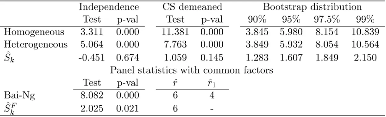
Table 1 reports the Hadri (2000) statistics –assuming either that long-run variance is homogeneous or heterogeneous – and the ^Sk statistic in Harris, Leybourne and McCabe (2005). When the individuals are assumed to be cross-section independent, both versions of Hadri’s statistics lead to reject the null hypothesis of variance stationarity at the 5% level of signi…cance, while the

^

Sk statistic does not. Therefore, the application of these panel stationarity statistics produces contradictory results. However, it should be beard in mind that these results are based on the fact that individuals are independent. Computations in Pesaran (2005) reveal that this assumption is far from being satis…ed. Thus, Pesaran (2005) computes the statistic in Pesaran (2004) and obtains strong evidence that points to existence of cross-section dependence. As noted above, this might bias the analysis leading to obtaining wrong conclusions.

To get a feeling of the size of the cross-sectional dependence problem in the RER data, we have proceeded to compute the statistics in Pesaran (2004) and Ng (2006) to test the null hypothesis of independence among individuals. The ADF-type regression equation in which the statistic is based uses the t -sig criterion in Ng and Perron (1995) to select the order of the autoregressive correction with up to ten lags. The computation of the CD statistic in Pesaran (2004) gives CD = 68:043, which leads to reject the null hypothesis of independence. As for the statistic in Ng (2006), the whole sample of spacings can be splitted in two groups, where the break point is estimated at ^ = 15. The svr ( ) statistic for the whole sample –svrW _{(^) = 5:179, with p-value 0.000 –and for} the large sample –svrL(^) = 4:065, with p-value 0.000 –indicate that the null hypothesis of non-correlation is strongly rejected. The statistic computed for the small sample reveals that the null hypothesis cannot be rejected at the 5% level of signi…cance –svrS(^) = 5:179, with p-value 0.785. Therefore, we can see that there is evidence of cross-section correlation among the individuals of the panel data set. Furthermore, the fact that the break point is estimated at ^ = 15 implies that the proportion of correlation coe¢ cients that form the S group # = 0:10^ is small compared to correlation coe¢ cients in the L group, which indicates that pervasive cross-correlation is present amongst the individuals in the panel data sets, so that approximate factor models as suggested in Bai and Ng (2004a) can capture the cross-section dependence in better way.

lead to erroneous conclusions, so that cross-section dependence has to be accounted for when testing the null hypothesis of panel stationarity. As mentioned above, in this paper we have dealt with cross-section dependence in three di¤erent ways. First, we have removed the cross-section mean, which does not change previous conclusions, i.e. we strongly reject the null hypothesis of variance stationarity using the Hadri (2000) statistics while it is not rejected when using the ^Sk statistic – see results reported in the columns labelled as CS demeaned in Table 1. Note that this approach is equivalent to assuming that there is one stationary common factor that a¤ects the individuals in the same way, which might be restrictive in practice. Second, we have computed the Bootstrap empirical distribution of the statistics following Maddala and Wu (1999) using 20,000 replications – we o¤er the percentiles of interest in Table 1. In this case, we …nd strong evidence in favor of the PPP hypothesis when using the (homogeneous long-run variance) Hadri’s statistic and the ^Sk statistic, since the null hypothesis of variance stationarity cannot be rejected even at the 10% level of signi…cance. When heterogeneous long-run variance is assumed in the computation of the Hadri (2000) statistic, the null hypothesis cannot be rejected at the 5% level, although it does at the 10% level. However, the statistic in Ng (2006) has shown that cross-section dependence among individuals is pervasive, so cross-section dependece should be better captured using approximate common factor models.

Finally, Table 1 presents the panel data stationarity statistics in Bai and Ng (2004a), and Harris, Leybourne and McCabe (2005) that consider the presence of common factors to model the cross-section dependence. In both cases, the number of common factors (r) has been estimated using the panel BIC information criterion in Bai and Ng (2002) with up to six common factors. The approach in Bai and Ng (2004a) allows us to investigate the source of stationarity separately, i.e. we can test the null hypothesis of stationarity for the idiosyncratic and estimated common factors. In contrast, the proposal in Harris, Leybourne and McCabe (2005) tests the null hypothesis of joint stationarity in both common factors and idiosyncratic disturbance terms. Note that in both situations the estimated number of common factors (^r) achieves the maximum number permitted – we increased the maximum number of common factors, but it was reached as well. We essayed other information criteria than the panel BIC in Bai and Ng (2002), i.e., ICp2(k) and ICp2(k) in

Bai and Ng (2002), and the number of estimated common factors always reached the maximum allowed. When the usual BIC information criterion, denoted as BIC3(k) in Bai and Ng (2002), was

used, the estimated number of common factors was less than the maximum permitted. However and as noted in Bai and Ng (2002), this information criterion may perform well for some but not all con…gurations of the parameters. Given the number of individuals that is considered in our study we have decided to use six common factors in the analysis, although the number of common factors might has been over-estimated by the panel BIC information criterion. Let us …rst focus on the Bai and Ng (2004a) statistic. The KPSS statistic applied to each estimated common factor reveals that there are ^r1 = 4 common stochastic trends, since the null hypothesis of variance stationarity can be rejected at the 5% level of signi…cance. The other two common factors are characterized as variance stationary. The panel data variance stationarity statistic computed using the idiosyncratic disturbance terms indicates that the null hypothesis is strongly rejected – the mean and variance required to compute this statistic are obtained by simulation. Therefore, both idiosyncratic and common factor components lead to reject the PPP hypothesis. This conclusion is also reached when using the ^SF

k statistic, since the joint null hypothesis of variance stationarity of the idiosyncratic and common factor components is rejected at the 5% level of signi…cance.

To sum up, the computations that have been carried out indicate that contradictory results are obtained depending on the way that section dependence is accounted for. When cross-section demeaned data is used, the Hadri (2000) and ^Sk statistics report contradictory results. Nevertheless, in our case the application of cross-section demeaning has been shown to be useless, provided that it implies assuming that there is only one stationary common factor, when in fact we have …nd more than one. The use of the bootstrap distribution points to the ful…lment of the PPP hypothesis, regardless of the statistic that is used. Notwithstanding, this conclusion might be a¤ected by the presence of common factors, which now is known to bias the analysis to conclude in favor of variance stationarity – see Banerjee, Marcellino and Osbat (2004, 2005). When common factor framework is used, we have not been able to …nd support for the PPP hypothesis ful…lment. This result is in accordance with most of previous evidence in the literature cited above, which implies that the PPP hypothesis is not satis…ed for the seventeen OECD countries that have been considered in the analysis.

3.2 Panel data stationarity tests with structural breaks

Previous analysis has not considered the presence of structural breaks, which might imply mislead-ing conclusions about the stochastic properties of the panel data set. In this section we consider this feature. There are some proposals in the literature that allow for the presence of structural breaks when testing the PPP hypothesis –see Perron and Vogelsang (1992), Hegwood and Papell (1998), and Papell (2002). In this section we address the robustness of previous conclusions in the presence of multiple structural breaks using the statistics described in Section 2.

We have estimated the number and position of the structural breaks using the procedure in Bai and Perron (1998) setting mmax= 5 as the maximum number of structural breaks –this maximum was never attained. The number of break points has been selected with the sequential approach in Bai and Perron (1998) – the level of signi…cance is set at the 5% level. The estimated break points are used to compute the statistics in Carrion-i-Silvestre, del Barrio-Castro and López-Bazo (2005), and Harris, Leybourne and McCabe (2005). Panel A in Table 2 o¤ers the values for the individual KP SSi and Si;k statistics, as well as the estimated break points. We have also included the simulated critical values at the 10% and 5% level of signi…cance for the individual KPSS statistic. Note that critical values for the Si;k test are not required, since this statistic converges to the standard Normal distribution. Inspection of the individual statistics reveals that the null hypothesis of variance stationarity cannot be rejected in any case for the individual KPSS statistic, while it is rejected in seven cases when using the individual Si;k test at the 5% level of signi…cance. If we combine this information to de…ne panel data statistics and assume that individuals are cross-section independent, we conclude that the null hypothesis of panel stationarity cannot be rejected with either version of the Z ( ) test, whereas it is rejected if we base on the Sk test – see Panel B in Table 2. Notwithstanding, evidence of strong cross-section dependence has been found in the previous analysis, so that we should check if this assumption holds in this case.

In order to test the null hypothesis of cross-section independence we have computed the tests in Pesaran (2004) and Ng (2006). We have estimated an ADF-type regression equation that includes dummy variables to account for the presence of level shifts – the order of the autoregressive cor-rection is selected as described above. The CD statistic computed with the estimated residuals of the ADF equations indicates that the null hypothesis of cross-section independence is strongly

re-jected, since CD = 64:586. The computation of the statistic in Ng (2006) gives svrW(^) = 1:147 (p-value 0.874), svrL(^) = 6:423 (p-value 0.000) and svrS(^) = 0:587 (p-value 0.722), for the whole sample, and large and small groups, respectively, with ^ = 14. The statistics for the whole and small sample indicate that the null hypothesis of independence cannot be rejected at the 5% level of signi…cance. However, the hypothesis is strongly rejected for the individuals in the large group. Provided that the fraction of individuals in the small sample is small ^# = 0:103 , we have to conclude that cross-section correlation among individuals is pervasive, so that it should be taken into account when assessing the stochastic properties of the panel data set.

When cross-section dependence is addressed, either through cross-section demeaning or comput-ing the empirical distribution by means of parametric bootstrap, all panel data statistics indicate that the null hypothesis of variance stationarity cannot be rejected at the 5% level of signi…cance – however, note that the null hypothesis is rejected at the 10% level of signi…cance for the ^Sk statis-tic. This conclusion is reinforced by the ^SF

k statistic when working at the 5% level of signi…cance, although the null hypothesis is rejected at the 10% level – as above, the analysis allows for up to six common factors. Therefore, we have found strong evidence of stationarity in variance of the RER for the set of countries that have been considered using both versions of the Z ( ) test. In addition, stationarity in variance of the RER is supported by the ^Sk and ^SkF statistics when the level of signi…cance is set at the 5% level, although the null hypothesis of variance stationarity is rejected at the 10% level of signi…cance.

Our results are qualitatively di¤erent from Harris, Leybourne and McCabe (2005), who …nd no evidence of PPP hypothesis when applying panel stationary test with cross-section dependence and structural breaks. Nevertheless, we should bear in mind that their evidence and ours are based on the use of time series of di¤erent frequency. One possible reason for the discrepancy of research conclusions is the constrained framework imposed in Papell (2002), and maintained in Harris, Leybourne and McCabe (2005). Thus, our results are based on an unconstrained set up that does not restrict the real exchange rates to return to the levels previous to the episode of appreciation and depreciation of the U. S. dollar in the 1980s. Therefore, it would be the case that even in the case that real exchange rates were only a¤ected by one episode a¤ecting the dollar, the level to which RER returned after the episode ended was not necessarily the same as the previous one. It is worth mentioning that our framework retains the possibility that RER returned

to similar (although not equal) values to those previous to the dollar episode in the 1980s, since it accommodates the presence of multiple structural breaks. Furthermore, the investigation that has been conducted here reveals that RER are a¤ected by other features than the dollar appreciation and depreciation episode, features that should be taken into account when assessing their stochastic properties.

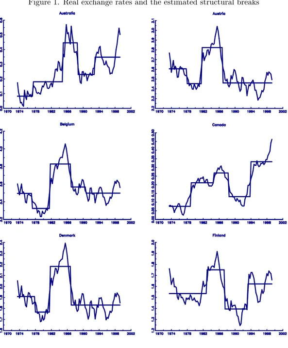
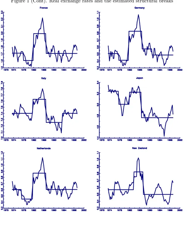
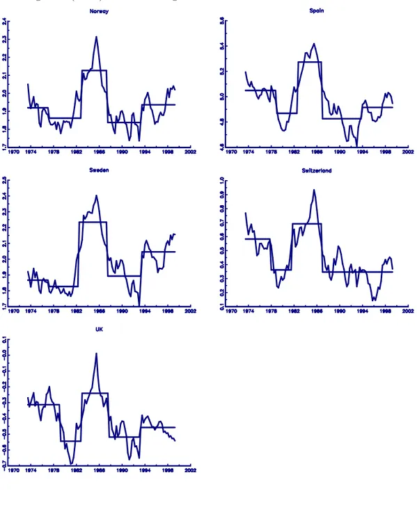
Panel A in Table 2 reports the estimated break points obtained from the Bai and Perron (1998) procedure, which are depicted in Figure 1. At least three breaks are found for each country (except New Zealand) with all breaks occurring during the period 1976Q3 to 1993Q2. From an historical point of view, this seems very reasonable with events such as oil price shocks, the rise and fall of U.S. dollar and the formation of European Monetary System (EMS). In fact, Papell (2002) identi…ed graphically three major regimes that are likely to have impacted the slopes of real and nominal exchange rates during the post-1973 era. The results in Table 2 reveal that in most cases, the …rst break occurred during the period 1976Q3 to 1978Q3, which may have resulted due to the oil price shocks in 1974. The second break took place at the beginning of 1980s (between 1981Q1 and 1982Q2), which clearly mimics the start of dollar’s appreciation. The third break con…rms the transition of dollar’s appreciation to depreciation during the period 1986Q2 to 1988Q1.5 Few countries (mostly European) experienced a fourth break occurring at the beginning of 1990s, which can be explained by the German reuni…cation and the formation of EMS. Thus European countries involved in the EMS carried out progressive abolition of any remaining capital controls among the European countries by 1990. In addition, the EMS crisis in September 1992 explains the estimated break points at the beginning of the 1990s. Thus, the exits of Italy and the UK from the exchange rate mechanism of the EMS re‡ect the detected structural breaks on the fourth and third quarter of 1993 for these countries, respectively. Furthermore, in August 1993 exchange rate bands of the EMS were increased to 15% , which was followed to the adherence of the prospective euro members to the Maastricht conditions on nominal convergence.

As can be seen, the procedure that has been applied in this paper allows the detection of the structural breaks that corresponds with the dollar episode in the middle of the 1980s, as well as it captures important features that have a¤ected most countries in the panel data set in the early

5_{For further discussion on the rise and fall of U.S. dollar and the determination of possible breaks in the slopes,}

1990s. These elements were not taken into account in previous analyses where testing for the stationarity in variance of the RER using panel data techniques was the main aim.

4

Half-life measurement

The PPP puzzle, which has intrigued researchers for many years and has devoted huge amount of contributions in the literature, is the apparent contradiction between the high persistence of shocks to RER (three to …ve years) and the high short-term volatility that exhibit (nominal and real) exchange rates. This feature has been investigated in a ‡urry of papers, which in most of them the persistence of the shocks is approximated by mean of half-life (HL) measures – the HL is usually de…ned as the number of time periods required for a unit impulse to dissipate by one half. The extent to which a shock to the RER lasts is a crucial question in the context of sticky-price versions of New Open Economy Macroeconomics models, since theories typically imply a length of half-life between one and two years. Rogo¤ (1996), while reviewing the empirical literature, reached to the consensus estimate of 3-5 year half-lives of PPP deviations.

Most of the empirical illustrations of HL calculation for RER are concerned with the time series estimation,6 and only few recent ones deal with panel data methods. For example, Choi, Mark and Sul (2006) focus on CPI-based annual real exchange rates and …nd that the HL to be 5.5 years (with a 95% con…dence interval ranges from 4.3 to 7.3 years) for a panel of 21 OECD countries during the post-1973 period. Murray and Papell (2005) put the HL to 3.55 years (with a 95% con…dence interval of 2.48 and 4.09 years) for 20 OECD countries during the post-1973 period applying the approximate median-unbiased (MU) estimation method in Andrews and Chen (1994). These analyses are based on the estimation of panel data models that restrict the autoregressive coe¢ cient to be homogeneous for all individuals in the panel data set.7 The main conclusion of these recent panel studies is that the …ndings of univariate methods are con…rmed, so that the PPP puzzle remains unsolved.

In this section we shed light on the PPP puzzle using the panel data framework developed in the earlier sections. To the best of our knowledge, no previous studies have examined this issue

6_{See Murray and Papell (2002) for a recent account based on univariate method.} 7

Although Choi, Mark and Sul (2006) and Imbs, Mumtaz, Ravn and Rey (2004) have both pointed out that inappropriate pooling across cross-sectional units may result in an upward bias in the estimated half-life, Chen and Engel (2005) …nd that it is not an important source of bias.

in a panel data framework while simultaneously considering the pervasive source of cross-sectional dependence and multiple structural breaks. Furthermore, the approach that has been followed here allows us to distinguish two di¤erent stochastic components, i.e. the idiosyncratic and the common factor components. This permits the computation of both idiosyncratic HL and common HL measures of persistence, which has not been previously calculated in the literature.

We have followed Murray and Papell (2002, 2005) in order to measure the persistence of the shocks. Thus, we have estimated an autoregressive speci…cation for the estimated idiosyncratic disturbance terms and the common factors, which are the ones that have been obtained from the model that incorporates multiple structural breaks. As above, the selection of the order of the autoregressive model is done using the t -sig information criterion in Ng and Perron (1995) with up to ten lags. It is well known that the OLS estimation method of autoregressive models produces biased estimates, which in turn causes biased measures of HL. In order to account for this estimation bias, we have estimated the parameters of the autoregressive models using the MU estimation method in Andrews and Chen (1994). In addition, the application of this procedure allows us to obtain con…dence intervals for the parameters, so that con…dence intervals for the idiosyncratic and common HLs can be established. The estimation of the HLs depends on the order of the autoregressive model that is used. When we are dealing with an AR(1) model the HL estimate can be directly computed as HL = ln (0:5) = ln (^M U), where ^M U denotes the autoregressive parameter. However, when the order of the autoregressive model is greater than one, the HL estimate has to be obtained from the impulse response function – see Murray and Papell (2002) for further details. In this case, M U will denote the sum of the autoregressive parameters.

Table 3 presents the MU estimates of M U as well as the HL measures based on these MU estimates for each individual. Despite of the point estimates, we report the 95% con…dence interval for ^M U and the corresponding HL measures. Panel A in Table 3 reports the computation for the idiosyncratic disturbance terms, while Panel B o¤ers the results for the common factors. Some remarks are in order. First, the estimates that have been obtained for M U, either for the idiosyn-cratic or the common components, are lower than the ones obtained in the literature. Furthermore, we can see that the upper limit of the 95% con…dence intervals is below one in all cases. This is because the approach that has been followed here distinguishes two sources of shocks –idiosyncratic and common shocks –as well as it considers the presence of multiple structural breaks. Therefore,

we account for two important features when estimating the autoregressive parameters that are well known to be potential sources of bias estimation. Second, the HL point estimates are below one year for both the idiosyncratic and the common components. This is in sharp contrast with most of previous estimates, where HLs computed using similar data set were estimated around 3 to 5 years. Moreover and except for Denmark, the con…dence intervals indicate that HL estimates are below 1.356 years for the idiosyncratic component, and below 1.573 years if we focus on the common factor component. Note that in all situations, the con…dence intervals are quite narrow and informative when compared to previous estimates in the literature (e.g., Murray and Papell (2002, 2005)).

One may argue that …nding evidence of shorter half-lives is not an interesting result since by allowing break points in the autoregressive framework inherently reduce the persistence measures. However, doing so will imply to assume that previous investigations on the stationarity in variance of the real exchange rates are based on misspeci…ed models. In this regard, previous literature that do not consider the presence of such breaks are obtaining biased estimates of the autoregressive parameters – see Perron and Vogelsang (1992) for an early example of the potential problem. Therefore, our results re‡ect the potential pitfall in which PPP panel data analyses that do not consider the presence of pervasive cross-section dependence and multiple structural breaks can simultaneously incur. More interestingly, our framework shed light on the PPP puzzle, as described by Rogo¤ (1996), the enormous short-term volatility of the real exchange rates with the extremely slow rate at which shocks appear to damp out.

To sum up, the evidence that has been reported in this section indicates that PPP panel data analyses focusing on post-Bretton Woods era should consider the presence of cross-section dependence as well as multiple structural breaks when computing HL measures. Otherwise, the estimated measures of persistence might be upper biased, leading to conclude that shocks are more persistent than they really are.

5

Conclusions

In this paper, we re-examine the null of stationary of RER for a panel of seventeen OECD developed countries taking into account both the presence of cross-section dependence and multiple structural breaks. The approach that is followed throughout the paper is ‡exible enough to accommodate large degree of heterogeneity with respect to the presence of multiple structural breaks. We have investigated the maintained assumption of cross-section independence in which most previous panel data RER analyses rely on. The statistics that have been computed show that pervasive cross-section correlation is present among individuals, which indicates that a factor structure might help to capture the cross-section dependence. Nevertheless, the analysis has applied di¤erent approaches to account for the presence of cross-section dependence to study the robustness of the conclusions. Results depend on whether structural breaks are considered or not, i.e., we …nd evidence sup-porting the stationarity in variance of the RER when structural breaks are allowed for, while non-stationarity in variance is found when structural breaks are omitted. As a by-product we have measured the persistence of the idiosyncratic and common shocks to the RER through the compu-tation of half-life measure. Our point estimates of half-life shed light on the PPP puzzle since they turn out to be less than one year for both the idiosyncratic and common factor components used in the analysis. Our results may be interesting in view of recent research that purport to shed light on PPP by exploiting recent advances in panel data econometrics.

References

[1] Andrews, D. W. K. and Chen, H. Y., 1994, Approximately Median-Unbiased Estimation of Autoregressive Models, Journal of Business and Economic Statistics 12, 187-204.

[2] Bai, J. and Perron, P., 1998, Estimating and testing linear models with multiple structural changes, Econometrica 66, 47-78.

[3] Bai, J. and Ng, S., 2002, Determining the number of factors in approximate factor models, Econometrica 70, 191-221.

[4] Bai, J. and Ng, S., 2004a, A New Look at Panel Testing of Stationarity and the PPP Hy-pothesis. Indenti…cation and Inference in Econometric Models: Essays in Honor of Thomas J. Rothenberg, Don Andrews and James Stock (Ed.), Cambridge University Press.

[5] Bai, J. and Ng, S., 2004b, A PANIC attack on unit roots and cointegration, Econometrica 72, 1127-1177.

[6] Baltagi, B. H., 2005, Econometric Analysis of Panel Data. John Wiley & Sons, Third Edition. [7] Baltagi, B. H., and Kao, C., 2000, Nonstationary Panels, Cointegration in Panels and Dy-namic Panels: A Survey. In Baltagi (Ed.) Nonstationary Panels, Cointegration in Panels and Dynamic Panels, Advanves in Econometrics, 15. North-Holland, Elsevier.

[8] Benerjee, A., 1999, Panel data units and cointegraiton: An overview, Oxford Bulletin of Eco-nomics and Statistics 61, 607-629.

[9] Benerjee, A., Marcellino, M. and Osbat, C., 2004, Some cautions on the use of panel methods for integrated series of macro-economic data, Econometrics Journal 7, 322-340.

[10] Benerjee, A., Marcellino, M. and Osbat, C., 2005, Testing for PPP: Should we use panel methods?, Empirical Economics 30, 77-91.

[11] Breitung, J. and Pesaran, M. H., 2005, Unit roots and cointegration in panels. Forthcoming in Matyas, L., Sevestre, P. (Eds.), The Econometrics of Panel Data, Klüver Academic Press.

[12] Caner, M. and Kilian, L., 2001, Size distortions of tests of the null hypothesis of stationarity: Evidence and implications for the PPP debate, Journal of International Money and Finance 20, 639-657.

[13] Carrion-i-Silvestre, J. L., T. Del Barrio, and E. López-Bazo (2002). Level Shifts in a Panel Data Based Unit Root Test. An Application to the Rate of Unemployment. Doct. Treball num. E02/79. University of Barcelona. http://www.ub.edu/ere/documents/papers/79.pdf.

[14] Carrion-i-Silvestre, J.L., Del Barrio-Castro, T. and López-Bazo, E., 2005, Breaking the panels: An application to the GDP per capita, Econometrics Journal 8, 159–175.

[15] Carrion-i-Silvestre, J. L. and Sansó, A., 2006, A guide to the computation of stationarity tests, Empirical Economics, forthcoming.

[16] Chang, Y. and Song, W., 2002, Panel unit root tests in the presence of cross-sectional depen-dency and heterogeneity, Mimeo., Rice University.

[17] Chen, S-S. and Engel, C., 2005, Does “aggregation bias" explain the PPP puzzle?, Paci…c Economic Review 10, 49-72.

[18] Choi, C-Y., Mark, N. and Sul, D., 2006, Unbiased estimation of the half-life to PPP convergence in panel data, forthcoming in Journal of Money, Credit and Banking.

[19] Cheung, Y. W. and Lai, K., 2000, On cross-country di¤erences in the persistence of real exchange rates, Journal of International Economics 50, 375-397.

[20] Choi, I., 2001, Unit root tests for panel data, Journal of International Money and Finance 20, 249-272.

[21] Coakley, J., and Fuertes, A.M., 1997, New panel unit root tests of PPP, Economics Letters 57, 17-22.

[22] Culver S.E., Papell, D. H., 1999, Long-Run purchasing power parity with short-run data: Evidence with a null hypothesis of stationarity, Journal of International Money and Finance 18, 751-768.

[23] Engel, C., 2000, Long-run PPP may not hold after all, Journal of International Economics 57, 243-273.

[24] Frankel, J.A., and Rose, A.K., 1996, A panel project on purchasing power parity: Mean reversion within and between countries, Journal of International Economics 40, 209-224. [25] Hadri, K., 2000, Testing for stationarity in heterogeneous panel data, Econometrics Journal

3, 148-61.

[26] Harris, D., McCabe, B., and Leybourne, S., 2003, Some limit theory for in…nite-order autoco-variances, Econometric Theory 19, 829-864.

[27] Harris, D., Leybourne, S., and McCabe, B., 2005, Panel stationarity tests for purchasing power parity with cross-sectional dependence, Journal of Business & Economic Statistics 23, 395-409. [28] Hegwood, N. D., and Papell, D. H., 1998, Quasi purchasing power parity, International Journal

of Finance and Economics 3, 279-289.

[29] Im, K-S., Lee, J., and Tieslau, M., 2005, Panel LM unit-root tests with level shifts, Oxford Bulletin of Economics and Statistics 67, 393-419.

[30] Imbs, J., Mumtaz, H., Ravn, M. O. and Rey, H., 2004, PPP strikes back: Aggregation and the real exchange rate, NBER Working Paper No. 9372.

[31] Kuo, B.-S. and Mikkola, A, 2001, How sure are we about purchasing power parity? Panel evidence with the null of stationary real exchange eates, Journal of Money, Credit, and Banking 33, 767-789.

[32] Kwiatkowski, D., Phillips, P.C.B., Schmidt, P.J., and Shin, Y., 1992, Testing the null hypoth-esis of stationarity against the alternative of a unit root: How sure are we that economic time series have a unit root, Journal of Econometrics 54, 159-78.

[33] Levin, A., Lin, C. F. and Chu, J., 2002, Unit Root Tests in Panel Data: Asymptotic and Finite-sample Properties, Journal of Econometrics 108, 1-24.

[34] Leybourne S. J. and McCabe B. P. M., 1994, A Consistent Test for a Unit Root, Journal of Business & Economic Statistics 12, 157-166.

[35] MacDonald, R., 1996, Panel unit root tests and real exchange rates, Economics Letters 50, 7-11.

[36] Maddala, G. S. and Wu, S., 1999, A comparative study of unit root tests with panel data and a new simple test, Oxford Bulletin of Economics and Statistics 61, 631-52.

[37] Moon, R. H. and Perron, B., 2004, Testing for unit root in panels with dynamic factors, Journal of Econometrics 122, 81-126.

[38] Murray, C. J. and Papell, D. H., 2002, The purchasing power parity persistence paradigm, Journal of International Economics 26, 1-19.

[39] Murray, C. J. and Papell, D. H., 2005, Do panels help solve the purchasing power parity puzzle?, Journal of Business & Economic Statistics 23, 410-415.

[40] Ng, S. and Perron, P., 1995, Unit root tests in ARMA models with data dependent methods for the selection of the truncation lag, Journal of the American Statistical Association 90, 268-281.

[41] Ng, S., 2006, Testing cross-section correlation in panel data using spacings, Journal of Business & Economic Statistics, 24, 12-23.

[42] O’Connell, P. G. J., 1998, The overvaluation of the purchasing power parity, Journal of Inter-national Economics 44, 1-19.

[43] Oh, K-Y., 1996, Purchasing power parity and unit root tests using panel data, Journal of International Money and Finance 15, 405-418.

[44] Papell, D., 1997, Searching for stationarity: purchasing power parity under the current ‡oat, Journal of International Economics 43, 313-332.

[45] Papell, D., 2002, The great appreciation, the great depreciation, and the purchasing power parity hypothesis, Journal of International Economics 57, 51-82.

[46] Papell, D. and Prodan, R., 2006, Additional Evidence of Long-run Purchasing Power Parity with Restricted Structural Change, Journal of Money, Credit and Banking 38, 1329-1350.

[47] Perron, P., 1989, The great crash, the oil price shock, and the unit root hypothesis, Econo-metrica 57, 1361-1401.

[48] Perron, P. and Vogelsang, T., 1992, Nonstationarity and level shifts with an application to purchasing power parity, Journal of Business & Economic Statistics 10, 301-320.

[49] Pesaran, M.H., 2004, General Diagnostic Tests for Cross Section Dependence in Panels, Cam-bridge Working Papers in Economics, No. 435, University of CamCam-bridge, and CESifo Working Paper Series No. 1229.

[50] Pesaran, H. M., 2005, A Simple Panel Unit Root Test in the Presence of Cross Section De-pendence, Cambridge Working Papers in Economics 0346, University of Cambridge.

[51] Rogo¤, K., 1996, The purchasing power parity, Journal of Economic Literature 34, 647-668. [52] Smith, V., Leybourne, S., Kim, T. H. and Newbold, P., 2004, More powerful panel data unit

root tests with an application to mean reversion in real exchange rates, Journal of Applied Econometrics 19, 147-170.

[53] Sul D., Phillips P. C. B. and Choi C. Y., 2005, Prewhitening bias in HAC estimation, Oxford Bulletin of Economics and Statistics 67, 517-546.

[54] Taylor, A.M., 2001, Potential pitfalls for the purchasing-power-parity puzzle? Sampling and speci…cation biases in mean-reversion tests of the law of one price, Econometrica 69, 473-498. [55] Wu, Y., 1996, Are real exchange rates nonstationary? Evidence from a panel-data test, Journal

of Money, Credit and Banking 28, 54-63.

[56] Wu, J-L., and Wu, S. 2001, Is purchasing power parity overvalued? Journal of Money, Credit and Banking 33, 804-812.

Table 1: Panel data variance stationarity test statistics without structural breaks

Independence CS demeaned Bootstrap distribution

Test p-val Test p-val 90% 95% 97.5% 99%

Homogeneous 3.311 0.000 11.381 0.000 3.845 5.980 8.154 10.839

Heterogeneous 5.064 0.000 7.763 0.000 3.849 5.932 8.054 10.564

^

Sk -0.451 0.674 1.059 0.145 1.283 1.607 1.849 2.150

Panel statistics with common factors

Test p-val r^ r^1

Bai-Ng 8.082 0.000 6 4

^ SF

k 2.025 0.021 6

-Table 2: Individual and panel data stationarity tests with multiple structural breaks Panel A: Individual statistics

Critical values KP SSi 10% 5% Si;k Tb;1i Tb;2i Tb;3i Tb;4i Australia 0.0213 0.059 0.069 -0.284 1976Q4 1984Q2 1988Q1 1992Q2 Austria 0.0305 0.100 0.126 2.326 1977Q2 1981Q1 1986Q2 Belgium 0.0362 0.063 0.076 1.838 1976Q3 1981Q1 1986Q2 1990Q1 Canada 0.0314 0.054 0.062 0.843 1978Q2 1984Q1 1987Q4 1993Q2 Denmark 0.0228 0.100 0.126 3.051 1977Q2 1981Q1 1986Q2 Finland 0.0365 0.076 0.091 1.017 1982Q2 1986Q4 1992Q3 France 0.0283 0.099 0.124 1.391 1977Q2 1981Q2 1986Q2 Germany 0.0369 0.062 0.074 2.341 1977Q1 1981Q1 1986Q2 1990Q2 Italy 0.0373 0.071 0.083 0.654 1981Q1 1986Q2 1992Q4 Japan 0.0422 0.100 0.128 -0.711 1977Q1 1981Q2 1986Q1 Netherlands 0.0372 0.101 0.127 1.987 1976Q3 1981Q1 1986Q2 New Zealand 0.0163 0.117 0.143 0.127 1983Q1 1986Q4 Norway 0.0283 0.055 0.062 0.706 1976Q3 1982Q2 1986Q4 1992Q4 Spain 0.0248 0.056 0.065 0.708 1978Q2 1982Q1 1986Q2 1993Q2 Sweden 0.0442 0.055 0.063 1.703 1976Q3 1981Q4 1986Q4 1992Q4 Switzerland 0.0253 0.099 0.125 2.053 1977Q2 1981Q1 1986Q2 UK 0.0406 0.055 0.063 0.153 1978Q3 1982Q2 1987Q1 1992Q3

Panel B:Panel Stationarity Tests

Independence CS demeaned Bootstrap distribution

Test p-val Test p-val 90% 95% 97.5% 99%

Z ( ) Hom. -2.237 0.987 -1.689 0.954 6.780 7.888 8.874 10.279

Z ( ) Het. -1.983 0.976 -1.921 0.973 6.313 7.464 8.548 10.002

^

Sk 1.965 0.025 -0.253 0.600 1.639 1.974 2.264 2.575

Panel Stationarity test with common factors

Test p-val ^r r^1

^

-T able 3: M edian-un biased -bas ed au toregress iv e p ar ame te r and H alf -l if e (i n y ear s) es ti mates for th e id io sy n crat ic an d common comp one n ts P anel A: Idiosy ncr a tic comp on en t ^M U parameter HL estimat es Con… de nce in terv al Con… de nce in terv al (95% lev el of con… de nce ) (95% lev el of con… de nce ) Lags P oin t estimate Lo w er limit Up p er li m it P oi n t es timate Lo w er limit U p p er limi t Aus trali a 0 0. 625 0.45 7 0.81 9 0.3 69 0.221 0.868 Aus tria 3 0. 702 0.53 0 0.85 3 0.4 84 0.275 1.003 Belgium 1 0. 480 0.31 0 0.66 0 0.2 41 0.181 0.388 Canad a 0 0. 711 0.52 1 0.85 6 0.5 08 0.266 1.115 Denm a rk 8 0. 775 0.52 4 0.93 1 0.7 03 0.271 3.187 Fi n lan d 3 0. 709 0.52 7 0.85 1 0.5 01 0.273 1.006 F ranc e 3 0. 647 0.45 5 0.79 1 0.3 70 0.229 0.685 Ger m a n y 3 0. 653 0.47 5 0.80 6 0.3 82 0.238 0.744 Ital y 4 0. 329 0.02 2 0.53 1 0.1 86 0.128 0.273 Japan 0 0. 699 0.55 6 0.88 0 0.4 84 0.295 1.356 Nethe rland s 0 0. 722 0.52 7 0.85 8 0.5 32 0.271 1.132 New Ze al an d 0 0. 591 0.37 2 0.75 4 0.3 30 0.175 0.614 Nor w a y 7 0. 300 -0. 040 0.50 8 0.1 79 0.120 0.257 Sp ai n 1 0. 735 0.59 3 0.87 0 0.4 99 0.320 1.138 Sw ede n 0 0. 738 0.56 4 0.87 8 0.5 71 0.303 1.332 Switze rland 3 0. 569 0.36 1 0.73 4 0.3 05 0.196 0.534 UK 0 0. 541 0.24 0 0.67 4 0.2 82 0.122 0.439 P anel B: Common factor comp onen t ^M U parameter HL estimat es Con… de nce in terv al Con… de nce in terv al (95% lev el of con… de nce ) (95% lev el of con… de nce ) F ac tor Lags P oi n t es ti mate Lo w er limit Upp er limit P oi n t es timate Lo w er limit U p p er limi t 1 4 0.485 0 .239 0.662 0.2 43 0.164 0.396 2 3 0.637 0 .485 0.762 0.3 61 0.243 0.559 3 1 0.682 0 .531 0.825 0.3 98 0.269 0.743 4 0 0.702 0 .533 0.859 0.4 90 0.275 1.142 5 0 0.689 0 .586 0.896 0.4 66 0.325 1.573 6 4 0.366 0 .050 0.574 0.1 97 0.132 0.320 The column lab ell ed as Lags d en o te s the n u m b er of lags th at has b een in clud ed in th e ADF -t y p e re gr es sion eq u a tion that is us ed to o b ta in the MU parameter es timates .