Greenhouse gases exchange over and within a tropical forest in Africa

Department for innovation in biological, agro-food and forest systems

PhD Course

Forest Ecology

XXIV cycle 2009 – 2011

G

REENHOUSE GASES EXCHANGE OVER AND WITHIN

A TROPICAL FOREST IN

A

FRICA

(AGR/05)

Course coordinator: Prof. Paolo De Angelis

__________________________

Tutor: Prof. Riccardo Valentini

__________________________

Co-tutor: Dr. Gerardo Fratini

__________________________

Co-tutor: Dr. Paolo Stefani

__________________________

PhD student: Giacomo Nicolini

__________________________

Greenhouse gases exchange over and within

a tropical forest in Africa

II Giacomo Nicolini

III

C

Abstract V

Sommario VII

1 Introduction ... 1

1.1 Background on greenhouse gases... 1

1.2 Eddy covariance method ... 4

1.2.1 Theory and equations ... 6

1.2.2Eddy covariance raw data acquisition and processing... 9

1.3 Study site: Ankasa Forest Conservation Area, Ghana. ... 18

2 State of the art in micrometeorological trace gas flux measurements ... 20

2.1 Literature review of micrometeorological CH4 and N2O flux measurements... 21

2.2 Flux variability within and between ecosystem categories ... 23

2.3 Flux detection limits and sensors suitability ... 27

2.4 Performances with respect to soil enclosure methods ... 30

2.5 Discussions and conclusions on trace gas flux micrometeorological measurements. .... 31

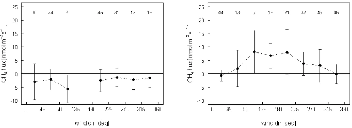
3 A preliminary assessment of below canopy methane fluxes in a tropical rain forest. ... 35

3.1 Introduction ... 35

3.2 Materials and methods... 36

3.2.1 Site description ...36

3.2.2 Eddy covariance measurement system...37

3.2.3 Eddy covariance data processing ...37

3.2.4 Methane flux detection limit of the eddy covariance system...38

3.3 Results ... 39

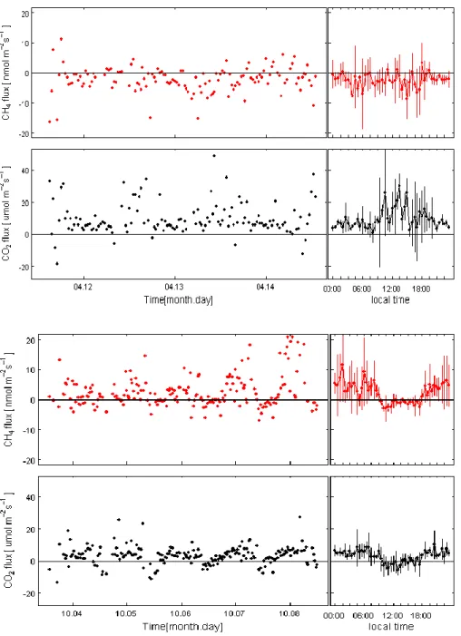
3.3.1 The magnitude and variability of energy, carbon dioxide and methane fluxes ...39

3.3.2 Consistency of methane fluxes estimates...41

3.4 Conclusions ... 42

4 The impact of the storage term on above canopy CO2 and CH4 fluxes ... 44

4.1 Introduction ... 44

4.2 Site and measurements ... 45

4.3 Calculation of the storage fluxes ... 46

4.4 Results ... 46

4.5 Conclusions ... 53

5 CH4 and CO2 fluxes over a tropical forest in Africa... 56

IV

5.2 Measurement site, set-up and meteorological conditions ... 56

5.3 Data processing and screening ... 59

5.4 Results ... 60

5.4.1 Variability of CO2 and CH4 mixing ratio... 60

5.4.2 Energy and scalar fluxes ... 61

5.4.3 Data screening and measurement quality... 64

5.4.4 Flux footprint ... 66

5.5 Discussions and conclusions ... 67

6 General discussions...70

References ...72

V

Abstract

Within the last years progress has been made in measuring trace gas fluxes at landscape scales thanks to development in technologies and their use in micrometeorological methods. However, there are still open questions. Two main factors contribute to limit the ability to precisely quantify annual or seasonal budgets of these gases. First, their net biosphere/atmosphere exchange rate is controlled by many biological, chemical and physical ecosystem parameters resulting in a very high temporal and spatial variability of fluxes. Second, such gases have a quite low atmospheric concentration, at least compared with CO2, which, in combination with

their small flux rates, makes the flux measurement a challenging technological achievement. As a consequence, exhaustive assessment requires high spatial resolution and continuous long-term monitoring. Eddy-based measurements can improve the accuracy of trace gas flux estimates, detect the short-term variability of fluxes, lead to estimates from site to landscape scales and provide a useful tool to parameterize and validate process-oriented models.

Measurement reliability can be optimized by an accurate field campaign and an appropriate data processing but assessing the source-sink mechanism in time and space, and the sources and magnitude of errors of estimates is still challenging.

Furthermore, some geographical areas like Africa still remain uncovered form such studies, while more information on trace gas exchange over these regions, especially within key ecosystems like forests, are becoming today urgent to properly understand the global cycles of trace gases.

In this thesis the fluxes of the two main greenhouse gases, CH4 and CO2, are measured by means

of the eddy covariance technique in the rainforest of Ankasa in Ghana.

Since tropical rainforests play a prominent role in the global carbon and methane cycle, flux dynamics are investigated both over and within the forest canopy.

But while for CO2 the measurement routine is more consolidated, here the potential of the EC

techniques in measuring CH4 flux in such complex ecosystem is also evaluated.

To achieve these results, the working plan was structured in several phases.

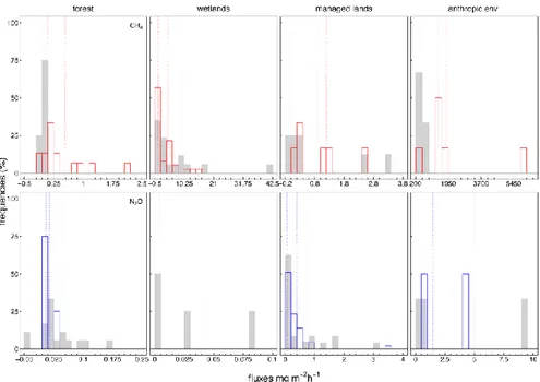
As EC methane flux measurements is a rather recently topic, a preliminary meta-analysis by which the state of the art in trace gas fluxes studies on global scale is reviewed to focus on needs and gaps on observations and to highlight strength and weakness of measurement techniques. This result is presented in chapter 2. In this analysis also nitrous oxide fluxes are included but filed works on this gas is not reported here as represent the aim of future works. The available data coming from different biomes it is synthetized grouping ecosystems in the broad categories (forest, managed land, wetlands and anthropic environments). Range of emissions across biomes according to different techniques are discussed along with flux detection limits and comparison with soil chamber measurements. Finally some considerations about future research directions and gaps on observation ore offered.

A challenging task like measure below canopy methane fluxes is reported in chapter 3. Beyond the high spatial and temporal variability of CH4 sources, such kind of estimates is further

VI

two short measurement campaign, executed during the dry and wet season in a periodically swamped area near the main tower. The feasibility of the approach is evaluated with the aim of programming a longer sampling and comparing results with concurrent soil chamber measurements.

In chapter 4 is reported an investigation on CO2 and CH4 storage fluxes and how much they

impact on above canopy fluxes. For CO2 results are based on one year dataset of continuous

profile measurements while for CH4 24 hours samplings were performed over different seasons.

The relation between the two storages and between storages and some controlling environmental variables are explored with the aim of either properly correct the above canopy flux, test the magnitude and the suitability of such corrections and eventually parameterize the storage flux trend.

In chapter 5, CH4 and CO2 fluxes measurement over the forest canopy is reported. This is the

core of the thesis and a deeper analysis is performed. The sampling has regarded several months covering the shift from the wet to dry season. Prior to the reported measurement period, further campaigns have been conducted but instrument failures, energy cut-offs and other technical problems have been prevent reliable results. Anyway such effort was useful to individuate the weakness of the measurement system and assess the methane gas sensor performances. In fact, a newly developed open path sensor was used and application experiences are currently being evaluated.

Beyond the fluxes quantification here it is reported the seasonal trend analysis of fluxes, the footprint analysis to localize the source regions, the error assessment and the quantification of the minimum detectable flux. Then a carbon balance for the analysed period is computed.

VII

Sommario

Negli ultimi anni sono stati compiuti numerosi progressi nella stima dei gas-traccia su scala ecosistemica grazie allo sviluppo di tecnologie innovative e al loro utilizzo tramite tecniche micrometeorologiche. Tuttavia, ci sono ancora aspetti che devono essere chiariti.

Due fattori principali contribuiscono a limitare la capacità di quantificare esattamente i bilanci stagionali o annuali di questi gas. In primo luogo, il loro tasso netto di scambio tra biosfera e atmosfera è regolato da molti parametri biologici, chimici e fisici e ciò determina un’ alta variabilità spaziale e temporale dei flussi. Inoltre, questi gas hanno delle basse concentrazioni atmosferiche (rispetto a quella della anidride carbonica) che, assieme a basse intensità di flusso, rendono la loro misura una sfida tecnologica. Di conseguenza, una valutazione esauriente richiede misure in continuo e con un’ ampia risoluzione spaziale.

Le misure basate sulla tecnica dell’ eddy covariance (EC) possono migliorare l’accuratezza di queste stime integrando la variabilità a breve termine dei flussi, fornendo stime su ampia scala e dati necessari alla parametrizzazione e validazione di modelli process-oriented.

L’affidabilità delle stime può essere ottimizzata da una campagna di misura accurata e un attento processamento dei dati. Tuttavia la valutazione del meccanismo di assorbimento/emissione e degli errori di stima presentano ancora ampi margini di studio.

Inoltre alcune aree geografiche come l’Africa sono poco interessate da questi studi nonostante il ruolo fondamentale che i loro ecosistemi, in particolare le foreste, svolgono nel bilancio globale del ciclo del carbonio.

Questa tesi riguarda lo studio dei flussi di metano (CH4) e anidride carbonica (CO2) misurati

nella foresta tropicale di Ankasa in Ghana tramite la tecnica dell’eddy covariance. Le misure sono state effettuate sia sotto che sopra lo strato delle chiome. Sono state inoltre valutate le potenzialità di questa tecnica nel misurare CH4 su ecosistemi complessi.

Per raggiungere questi obiettivi, il lavoro è stato articolato in fasi diverse.

Le misure EC di CH4 rappresentano un aspetto recente nello studio dei gas serra, quindi è stata

effettuata una meta-analisi preliminare attraverso la quale è stato possibile conoscere lo stato dell’arte di queste misure su scala globale, individuare le aree che maggiormente necessitano di osservazioni ed infine evidenziare i pro e i contro della tecnica. Il risultato di questa analisi è riportato nel capitolo 2. Qui viene incluso anche un altro gas traccia, il protossido di azoto (N2O),

ma le misure di questo gas non vengono ulteriormente trattate in quanto sono l’oggetto di un lavoro in fase di sviluppo. I dati raccolti tramite ricerca bibliografica, sono stati raggruppati in 4 grandi categorie di ecosistemi (foreste, terreni agricoli, zone umide e ambienti antropizzati). Per ogni categoria viene discusso: il range delle emissioni, il minimo flusso misurabile rispetto alla tecnica micrometeorologica adottata e il confronto con i risultati ottenuti con la tecnica delle camerette di accumulo al suolo. Infine vengono proposte alcune considerazioni sullo sviluppo di ricerche future e sulla necessità di aumentare il numero delle osservazioni.

La misura dei flussi di CH4 sotto chioma è riportata nel capitolo 3. Oltre che per l’alta variabilità

spaziale e temporale delle emissioni, questo tipo di misure è ulteriormente complicato dalla complessa turbolenza che si sviluppa tra i fusti degli alberi. In questo capitolo sono riportati i risultati di due campagne di misura eseguite su un’area periodicamente inondata, situata nei

VIII

pressi della stazione principale. La prima è stata condotta durante la stagione secca, la seconda in quella umida durante un periodo di inondazione. Oltre a valutare l’entità dei flussi e l’applicabilità della tecnica, questo esperimento è stato eseguito con lo scopo di programmare un campionamento più lungo e confrontare i risultati con stime effettuate al suolo con le camerette. Nel capitolo 4 è riportata un’analisi dello storage di CO2 e CH4 e di quanto esso contribuisca ai

flussi misurati dalla torre al disopra delle chiome. Per la CO2 i risultati sono basati su un anno di

misurazioni in continuo del profilo verticale lungo la torre. Per il CH4 sono stati effettuati

campionamenti di 24 ore durante tre campagne di misura in stagioni differenti. E’ stata esaminata la relazione tra i due storage e tra questi e alcune variabili ambientali con lo scopo di correggere adeguatamente i flussi sopra chioma, testare la portata e l’intensità di queste correzioni ed eventualmente parametrizzarne il trend.

Il capitolo 5 descrive la stima dei flussi di CH4 e CO2 effettuata al disopra dello strato delle

chiome tramite la tecnica dell’eddy covariance. Il campionamento è stato eseguito per diversi mesi durante il passaggio dalla stagione umida a quella secca. Nel periodo precedente alle misurazioni si sono verificati problemi di natura tecnica che hanno reso il dataset inutilizzabile. Tuttavia questo ha permesso di individuare i punti deboli del sistema e ottimizzare le prestazioni del sensore di CH4. Infatti lo strumento utilizzato per la misura delle concentrazioni di questo gas

è stato commercializzato solo di recente e la sua applicazione in campo è attualmente in fase di valutazione.

Oltre alla quantificazione dei flussi e l’individuazione della loro area sorgente (footprint), è riportata un’analisi dei trend, una valutazione dell’errore di stima e del flusso minimo misurabile dal sistema. Infine è stato calcolato il bilancio netto del carbonio durante il periodo di misura.

1

1 Introduction

1.1

Background on greenhouse gases

Earth atmosphere (air) is a mixture of gases and particles constituted by three major components, nitrogen (N2), oxygen (O2) and argon (Ar), representing about the 99.9% of

atmosphere volume; three secondary components, water vapour (H2O), carbon dioxide (CO2)

and ozone (O3); and trace components such as methane (CH4), nitrous oxide (N2O) and

halocarbons (CFCs, HCFCs). Due to the great mobility of the atmosphere together with its internal mixing, the proportion of such gases is almost constant at any latitude and up to 100 Km of altitude. The big importance of the atmosphere, as well as its first kilometres (around 10) where meteorological phenomena take place, lie behind the absorption of the cosmic radiation (x, gamma and UVC) emitted by the sun. Without the ‘atmospheric filter’ such radiations could get down to the Earth surface destroying the biosphere.

Despite the big contribution in terms of volume, the principal atmospheric components are effectively transparent to solar radiations, both long-wave and short-wave (but they play a role on short-wave diffusion, see later). Secondary and trace gases, even if they represent around 1 ‰ of the atmosphere volume, control the absorption and re-emission of radiation energy. In particular, due to their tri-atomic molecular structure, they absorb radiation in certain wavelengths, mostly in the long-wave region. Each gas absorbs in a different spectral band and these bands do not overlap so, as they are mixed in the air, the absorption takes place within all the characteristic bands of radiation. Between these bands there are two main windows through which part of the radiation can pass without being absorbed. One is the short-wave window (0.3 < λ < 1.5 μm) crossed by the solar irradiation peak coming to the Earth, and the other is the long-wave or infrared window (8 < λ < 14 μm) permeable to the Earth radiative emission going back towards the atmosphere (Fig. 1.1).

This selective absorption mechanism is universally known as green-house effect: the atmosphere, allowing short-wave incoming radiation to pass and absorbing most of the long-wave outgoing radiation, keeps the Earth temperature warmer than surrounding air.

The energetic balance of the Earth–atmosphere system with the external space is hence performed through this air mass that envelops the terrestrial surface, which has the clouds top as external frontier. To see the importance of this air layer, and of the green-house effect, let’s consider a simplified version of terrestrial energetic balance model:

4 0 4 4 ) 1 )( 1 ( P m E E T B A T       [1.1]

where 0 = 1.38·103 W m-2 is the energy flux density from the sun (solar constant), A ≈ 0.3 is the planetary albedo contribution (mainly due to clouds reflectance), B ≈ 0.2 is the atmospheric absorption contribution,  = 5.67·10-8 W m-2 K-4 is the terrestrial emittance, Em = 0.9 is the atmospheric emissivity and Tp = 255 K is the planetary temperature. Solving this

2 model we get a value of 291 K (18 °C), close to the measured mean terrestrial temperature of 288 K.

Figure 1.1. Left side: absorption bands in the Earth's atmosphere (middle panel), for major GHG (lower panel) and their impact on both solar radiation and up-going thermal radiation (top panel). The sun emissions peak is in the visible region (next to the short-wave window absorption band), emissions from the Earth vary with temperature, latitude and altitude peaking in the infrared (next to the long-wave window). Absorption bands are determined by the chemical properties of the gases, Rayleigh scattering represent the aerosol contribution. Right side: global average abundances of the major GHG. These gases account for about 96% of the direct radiative forcing by long-lived greenhouse gases since 1750. The remaining 4% is contributed by minor halogenated gases [http://www.esrl.noaa.gov/gmd/aggi/index.html].

If, for example, green-house gases (GHG) drastically diminish resulting in a lower atmospheric emissivity Em = 0.4 – 0.5, TE would drop down to -5 – 0 °C, causing a freezing of the Earth crust. On the contrary, a GHG increase causing the atmosphere to become like a black body (Em = 1), would correspond to an Earth surface mean temperature rising up to 23 °C, dangerously compromising life of all vegetal and animal species.

The evolution and the current composition of the atmosphere is strictly linked not only to the origin of our planet and to its geology, but also to the life forms that are born and evolved on it. Hence it is natural believe that its characteristics can change in the future in relation to the evolution of the biosphere, and in particular of the human species.

Historical changes in the atmosphere composition are reconstructed by analysing air bubbles within cores extracted from ice, wetlands and lakes. The trend for the last 30 years is showed in figure 1.1. Up to mid 1700, CO2 concentration was in the range 280 ± 20 ppm. During the

industrial era it rose roughly exponentially to 367 ppm in 1999 and up to 379 ppm in recent years [Le Treut, et al., 2007]. Carbon dioxide has increased from fossil fuel use in transportation, manufacture, gas flaring and cements production. Deforestation releases CO2

and reduces its uptake by plants. CO2 is also released during land use changes, biomass

burnings and natural biomass decomposition.

Direct atmospheric measurements since 1970 have also detected the increasing atmospheric abundances of methane and nitrous oxide. CH4 abundance was constantly around 700 ppb

until the 19th century, then a steady increase brought CH4 abundances to 1745 ppb at the end

non-3 CO2 GHG in the atmosphere today [Montzka et al., 2011]. Methane has increased as a result

of human activities related to agriculture, natural gas distribution and landfills. It is also released from microbial processes (methanogens) that occur in soil, sediments, wetlands and water bodies [Davidson and Shimel, 1995, Flechard et al., 2007]. At present N2O abundance

is 19% higher than pre-industrial levels and has increased at a mean rate of 0.7 ppb yr-1 during the past 30 years, passing from 314 ppb in 1998, 319 ppb in 2005 to 322 ppb at present [Le Treut, et al., 2007; Montzka et al., 2011]. Nitrous oxide is also emitted by human activities such as use of fertilizers in agriculture and fossil fuel burning. About 70% of the total amount of N2O emitted from the biosphere derives from soils [Mosier et al., 1998]. Oceans also

release N2O.

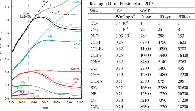
Radiative forcing (RF) is used to assess and compare the anthropogenic and natural drivers of climate change and it has proven to be particularly applicable to the assessment of the climate impact of GHGs as it can be linearly related to the global mean surface temperature change [Ramaswamy et al., 2001]. RF is computed basing on GHG concentration rate of change relative to 1750’s values and its efficiency in absorbing available infrared radiation. As reported by Montzka et al. [2011], by 2009 the increase in non-CO2 GHGs contributed a

direct radiative forcing of 1.0 W m-2, 57% of that from CO2, half of which (0.5 W m-2) is due

to CH4. In figure 1.2 GHGs current RF and projection are reported.

Table 1.1. GWPs of some GHGs. Readapted from Forster et al., 2007

GHG RF GWP

Wm-2ppb-1 20-yr 100-yr 500-yr

CO2 1.4 105 1 1 1 CH4 3.7 104 72 25 8 N2O 3.03 103 289 298 153 CCl3F 0.25 6730 4750 1620 CCl2F2 0.32 11000 10900 5200 CClF3 0.25 10800 14400 16400 CBrF3 0.32 8480 7140 2760 CCl4 0.13 2700 1400 435 CHF3 0.19 12000 14800 12200 CH2F2 0.11 2330 675 205 SF6 0.52 16300 22800 32600 NF3 0.21 12300 17200 20700 CF4 0.10 5210 7390 11200 C2F6 0.26 8630 12200 18200

Figure 1.2. Left side: radiative forcing derived from observed and projected abundances of long-lived gases (LLGHGs). Projections are made either assuming constant future emissions at 2008 levels and 80% cuts off.

Future forcing from the sum (black lines) of changes in CO2 (blue lines) and the sum of non-CO2 LLGHGs (red

lines). These sums is shown for different emission scenarios [see Montzka et al., 2011 for further detail].

To compare the impact of different GHGs on climate change, the global warming potential (GWP) index is used. It is based on the time-integrated global mean RF of a pulse emission of

4 1 kg of some compound relative to that of 1 kg of CO2, taken as a reference [Forster et al.,

2007]. Usually, non-CO2 emissions are multiplied by 100-yr time horizon GWPs to give CO2

-eq emissions. Despite their minor abundance, the global warming potentials of CH4 and N2O

are significantly higher than that of CO2, 25 and 298 times respectively.

As a consequence, to properly managing future intervention on climate forcing and improve scientific knowledge, non-CO2 gases must be given due consideration, as also reported by

Montzka et al. [2011]. Non-CO2 gases currently account for 1/3 of the total CO2-eq emissions

and 35–45% of total climate forcing from all GHGs, hence cuts in their emissions could substantially reduce future climate forcing. Act on shorter-lived non-CO2 gases emissions,

primarily on CH4 as it accounts for half of their total climate impact, can cause a rapid

decrease in the actual radiative forcing, otherwise impossible from cutting CO2 emissions

alone. On the other hand, such a quick response could not be achievable without concurrent substantial decreases in CO2 emissions. The stabilization of climate forcing will be

successfully achieved only with progresses in scientific research that enhance our understanding in the action-reaction mechanism of natural GHG fluxes on climate change and that improve our ability to properly quantify both natural and anthropogenic GHG fluxes.

1.2

Eddy covariance method

The eddy covariance (EC) technique is a micrometeorological method for measuring exchange of energy, momentum and mass (e.g. GHG) between a surface and the atmosphere. When this surface is horizontally uniform and flat the net exchange become mono-dimensional and the vertical flux density can be calculated as the covariance (see Sect. 1.2.1) between the turbulent fluctuation of vertical wind speed and the quantity of interest. This methods was originally proposed around the 1950 [Montgomery, 1948; Swinbank, 1950], the first measurement of a gas flux, CO2, is dated back to early 1970s [Desjardins, 1974] and the

first applications over forest were made after 1980s [Wesely et al., 1983; Fan et al., 1990; Valentini et al., 1991].

Mean flux across any plane implies correlation between the wind component normal to that plane and the entity in question, hence in their covariance there is a direct measure of the flux [Kaimal and Finnigan 1994]. Except for the first few millimetres of the atmosphere close to the earth surface, turbulent transport is the most important process in the exchange of energy and matter.

The turbulent motion of any variable ξ like e.g. the wind components (along a right-handed coordinate axes x, y and z respectively) u, v, w, the potential temperature θ, the mean specific humidity q or the gas concentration c, can be expressed as the sum of its mean component and the turbulent (fluctuation around the mean) component. Thus by the Reynolds decomposition we get ) ( ' ) (t   t    [1.2]

where  represent the average of the time dependent variables and ' t( ) its fluctuating part. The mean part within the averaging period T, is computed as

5



Such decompositions (and the following derivations) requires some averaging rules (Reynolds postulates) 0 '  I ' '       II      III [1.4]   a a  IV        V

These relations are theoretically obtained by ensemble averaging, i.e. averaging over many realizations under identical conditions [Kaimal and Finnigan, 1994]. Though in practice this is impossible given the natural variation of atmospheric conditions so the ensemble averages have to be approximated by averages over time, as the "ergodic" hypothesis asserts [Kaimal and Finnigan, 1994]. To satisfy this assumption, the fluctuations must be statistically stationary over the averaging period.

Turbulence in the atmosphere can be generated by mechanical production and buoyancy. The relative strength of both processes controls the vertical extent of turbulence.

The atmospheric boundary layer (ABL) is the part of the atmosphere that is directly influenced by the presence of the earth’s surface and respond to surface’s forcings with a timescale of about one hour or less [Stull, 1988]. This forcings include frictional drags, heat transfer, evaporation, transpiration, gas emissions and flow distortions induced by the terrain. The thickness of this layer is time and space dependent and varies from hundreds of meters to a few kilometres. The lowest 10% of the ABL is called surface (boundary) layer (SL). Fluxes in this layer can be considered approximately constant with height and the atmospheric turbulence is the primary way of transport. EC measurements are typically made at some height in the SL, which has a thickness of about 20-50 m in unstable atmospheric stratifications and 10-30 m under stable stratification [Stull 1988; Aubinet et al., 2012], and can be considered representative of the underlying surface.

The turbulent structure of the SL can be evaluated by several parameters. Following the theory expressed by Monin and Obukhov [1954] the main characteristics of the turbulence are described by the buoyancy parameter g/



The friction velocity is a generalized velocity dependent on surface nature and wind intensity representing the strength of wind stress. It may be usefully defined by [Foken 2008]





6 where u and w are expressed in m s-1.

The Monin-Obukhov length is given in meters by

' ' 3 *    w g u L [1.6]

where κ is the von Karman constant often set to 0.4 [Kaimal and Finnigan 1994].

The non-dimensional ratio ζ of height z to the scaling length L is often used to discriminate between atmospheric stability conditions

  

representing the relative importance of mechanical production (u*) and buoyancy (g  ). Generally ζ is negative in unstable atmosphere and positive when it is stable. Despite there are no fixed threshold values some classifications are proposed, one of which is reported in Table 1.2

Table 1.2. Surface layer stratification basing on the stability parameter ζ = z/L. Modified from Foken [2008].

stratification remark ζ unstable independent from u*

free convection -1 > ζ dependent from u*

mainly mechanical turbulence -1 < ζ < 0 neutral dependent from u*

purely mechanical turbulence ζ ≈ 0 stable dependent from u*

mechanical turbulence slightly damped by temperature stratification

0 < ζ < 0.5 – 2

independent from z

mechanical turbulence strongly reduced by temperature stratification

0.5 – 1 < ζ

1.2.1 Theory and equations

To derive the ecosystem exchange of a trace gas it is needed to base on the conservation

equation of any atmospheric constituent, both scalar and vector, ξ:

        S u t d d d       ) ( ) ( [1.8] I II III IV

7 where ρd is the dry air density,  is the divergence









/ , / ,

/x  y  z

 , K is the ξ diffusivity and S is the

ξ source/sink intensity [Aubinet et al. 2012; Gu et al., 2012]. By this model we can see that

the sum of the rate of change of ξ (temporal variation, term I), its atmospheric transport (advection, term II) and molecular diffusion (flux divergence, term III), equals its production by a source or absorption by a sink (term IV). Considering ξ as a wind component (u, v, w) we get the conservation equation for the momentum, as a temperature (cpθ), the conservation equation for the heat, while considering ξ as a trace gas mixing ratio (e. g. χCO2, χH2O, χCH4) we

obtain the trace gas conservation equation.

Therefore, assuming that molecular diffusion can be neglected in comparison to turbulent mixing [Stull, 1988], the conservation equation of any gas s becomes

s s d s d S u t     ) (     [1.9]

Considering the continuity equation as there is neither a source or sink of dry air in the atmosphere 0 ) ( /   _d t u_d [1.10]

and applying the Reynolds decomposition and the averaging postulates (Eq. from [1.2] to [1.4]) we get s s d s d s d s d s d s d s d S z w y v x u z w y v x u t                        ''  ''  ''        [1.11]

Under ideal conditions [Stull, 1988; Kaimal and Finnigan, 1994] v andw _{are 0 as the}

measurement system is aligned along the mean wind direction (no horizontal gradients); the gas concentration is steady with time (steady state condition) hence its time derivative nullifies; the underlying surface is homogeneous an flat so horizontal gradients (horizontal advection and flux divergences) equal zero. These assumptions simplify the gas conservation equation to a balance between the vertical gas flux divergence (gradient of eddy covariance) and its biological source/sink

s s d _S z w _   '' [1.12]

Defining a control volume over a flat homogeneous terrain with thickness z spanning from 0 to h (the measurement height in m), and considering the gas measurement made at height h as representative of the whole underlying volume, it is possible to integrate Eq. [1.11] just with

8 respect to height (hence not horizontally) obtaining the gas budget equation i.e. the EC method equation s h s d s d h s d dz w F z w dz t       





where term I is the gas storage in the underlying airspace (present when steady state condition is not met), term II is the vertical advection at the measuring point results from dry air density changes, term III (w ''



exchange (NEE) generally expressed in μmol m-2 s-1.

Normally the vertical advection is negligible with respect to the other terms hence Eq. [1.13] is further simplified.

The storage change depends on the stability of the atmosphere. During unstable conditions (normal daytime condition), the gas concentrations are well mixed and the storage change is small, however, during stable conditions (typical at nigh), the gas concentrations accumulate due to suppressed vertical motion by buoyancy destruction and the storage change term can become significant. The storage flux (μmol m-2 s-1) is calculated as [Aubinet et al., 2001]



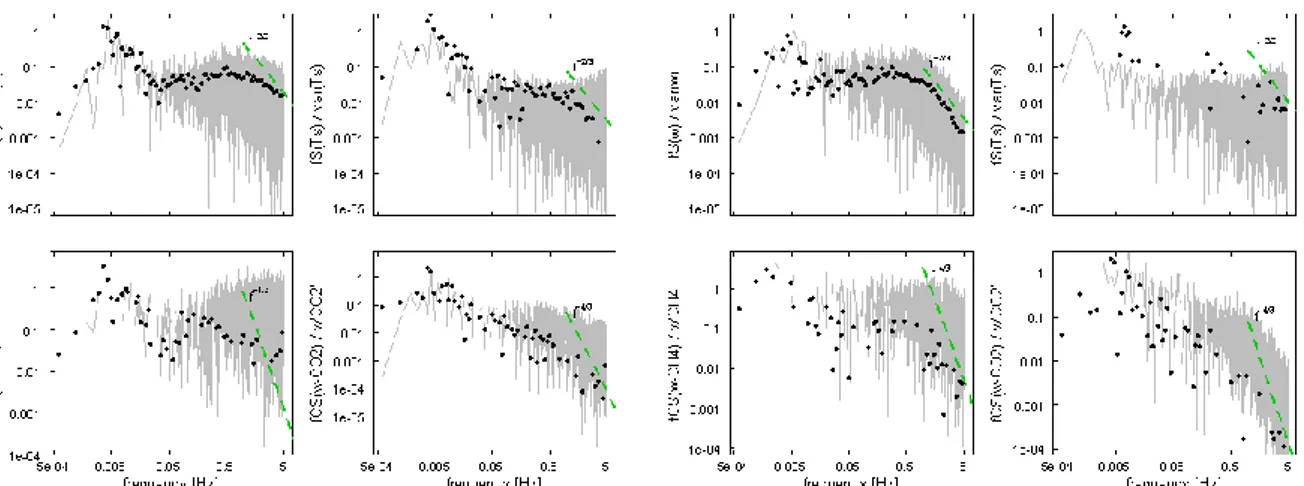
where Pa is the atmospheric pressure, Ta is the air temperature, R is the molar gas constant, c is gas concentration measured along the vertical profile of height h over an averaging period. The measured EC flux (term III of Eq. [1.13]) consists in a contribution of many eddies with different length scales, the turbulence spectrum [Stull et al., 1988]. The contribution of each eddy can be derived from the fast Fourier transform (FFT) analysis since each signals (wind velocity components, temperature or gas concentration) that contributes to the flux, can be seen as a linear combination of harmonic sine and cosine functions varying over a range of frequencies [Stull et al., 1988]. Assuming that signals are discrete time series consisting of N equally spaced data points (indexed by k = 0,..., N), then the available frequencies are n = 0, 1, ..., N-1 where n denotes the number of cycles within the averaging period. The contribution of each frequency to the variance of a quantity ξ is derived in two steps.

The signal ξ(kΔt) is split in several sine and cosine terms by the Fourier transform

) / 2 sin( 1 ) / 2 cos( 1 ) ( 1 1 N nk N N nk N n F N o k k N o k k     





for n = 0,…, nf, being nf the Nyquist frequency which is equal to N/2, then the spectrum of the quantity ξ is given by

9





with FRe, ξ being the real part and FIm, ξ the imaginary part of Fξ (n).

The co-spectrum of ξ and another signal as w, is derived in a similar way and is given by





The integral (or sum) over the whole frequency (f) range of the spectrum Sξ (n) and co-spectrum Cwξ (n), represent the variance and covariance (flux) of the signal [Kaimal and Finnigan 1994] ) ( ) ( 2 / 1 0 2 n S df f S N









Consequently, when the (co)spectra are plotted on linear axes, the area under the curve represents the (co)variance. Anyway the (co)spectra are usually plot on semi-log or log-log scale, maintaining the characteristic that the area under the curve represents the total (co)variance [Stull, 1988].

1.2.2 Eddy covariance raw data acquisition and processing

Data acquisition. The basic configuration of an EC system is a 3D sonic anemometer to

measure the three components of the wind velocity u, v and w (m s-1) and the sonic (then converted in ambient air) temperature (K or °C), a gas analyser measuring the trace gas and water vapour ambient concentration (mole fraction mol mol-1 or molar density mol m-3) plus a set of sensors to collect ancillary meteorological variables necessary to further analyse flux data.

Gas analysers are generally based on infra-red spectroscopy and are divided into two main categories. The open-path and the closed-path sensors. The former quantify scalar concentrations in situ, close to the point where the wind speed is measured. The latter are situated at some distance from this point and quantify scalar concentrations of air sucked down through a tube from an intake close to the anemometer [Haslwanter et al., 2009]. An

10 enclosed system aimed to maximize strength of both has been recently developed [Burba et

al., 2012].

Both the anemometer and the gas analyser must have a fast frequency response, i.e. sampling and collect data at rates up to 20 Hz (the anemometer sampling rate is normally twice). Such high frequencies are needed to ensure sample along all the frequency range of the turbulent spectrum. The gas sensor should have enough accuracy and precision to resolve gas concentration at ppb level (see Chap. 2). Such high frequency signals have to be averaged on a time period long enough to sample all the micro-turbulent spectrum time scale and at the same time ensure the steady state condition to be respected. Presently such integration period span from 15 to 60 minutes but is usually set to 30 min [Aubinet et al., 1999].

The meteo variables are directly acquired on a half-hourly scale and the usual set comprises global and net radiation (W m-2), photosynthetic photon flux density (PPFD, μmol m-2 s-1), air and soil temperature profile (K or °C), soil heat flux density (W m-2), precipitation (mm), air pressure (kPa), relative humidity (%), soil humidity profile (%).

The wind speed and gas concentration must be measured at a height above the vegetation that depends on the characteristics of the site. Normally the higher the measuring level the lower the required sampling rate because the size of the eddies increases (therefore their frequency decrease) moving away from the surface. However, with the increase of quote also increases the area over which the measured flux is integrated (source area), running the risk of sampling different source areas in case of inhomogeneous landscape. The extension of this area is defined by the footprint function, from which it is possible to calculate the fraction of the total flux due to a unitary element of surface positioned downwind within the source (see later). Normally the fetch (distance between sensors and the next soil/vegetation inhomogeneity) should be

) (

100 z d

d_fetch  _m [1.22]

where zm is the measurement height and d is the displacement height approximately taken as d

= 0.75 hc (the stand height). Traditional recommendation for zm is m

z z

d5 ₀  _m 100 [1.23]

where z0 is the roughness length approximately taken as z0 = 0.1 hc.

Once high frequency data have been collected and stored on half hour base, they need to be screened before flux computation occurs. Such operation necessitates of several computing steps and software routines are necessary.

Below is reported the processing steps that have been follow in this thesis and are implemented in EddyProTM

(LI-COR, Inc.), a free licence software for processing raw EC data to compute fluxes.

Despiking and statistical screening. Raw data despiking consists in detecting and

eliminating short-term outranged values in the time series. Usually spikes are one ore few consecutive values hence if more consecutive values are found to exceed the plausibility

11 threshold, they might be a sign of a real trend and don’t have to be eliminated. The statistical tests [Vickers and Mahrt, 1997] are amplitude resolution (insufficient sampling rate), drop-outs (short periods in which data are statistically different from the period average), absolute limits (values outside a plausible physical range), discontinuities (sharp series discontinuities that lead to semi-permanent changes), steadiness of horizontal wind (systematic reduction or increase in wind components series). Then, third (skewness) and forth (kurtosis) order moments are calculated on the whole time series and variables are flagged if their values exceed normal values.

Figure 1.3. Example of spike (red circle) and drop-out (dotted red line) on CO2 concentration time series.

Wind angle of attack and axis rotation (tilt correction). If the wind approaches the

anemometer with a an angle that deviates significantly from horizontal, the structure of some sonic anemometer can distorts the flow, resulting in inaccurate measurements. If the angles of attack calculated throughout the current averaging period exceed a pre-fixed threshold, data have to be corrected [Nakai et al., 2006].

As stated in the previous section, the reference coordinate system have to be aligned with the horizontal mean wind component (the x-axes parallel to u direction, the z-axes perpendicular to the mean stream flow and the y-axes perpendicular to the xz-plane) to respect the assumptions on the scalar conservation equation (Eq. [1.13]) i.e. negligible mean vertical wind component. Small errors in the alignment of the anemometer has big repercussion on fluxes estimate as the cross contamination of velocities that occurs with a nonaligned anemometer cause fluctuations in the longitudinal components of the wind appear as vertical velocity fluctuations and vice versa [Wilczak et al., 2001]. There are three methods for addressing anemometer tilting: the double rotation, triple rotation, and the planar fit method. In the double rotation method the first correction is the rotation around the z-axes to ensures that the coordinate system is oriented along the mean wind direction [Kaimal and Finnigan 1994]   sin cos 1 um vm u     cos sin 1 um vm v   [1.24] m w w1 

12 where um, vm, wm are the measured wind components and θ is the rotation angle defined as

          m m u v 1 tan  [1.25]

The second rotation is around the new y-axes until the mean vertical wind nullify









where u2, v2, w2 are the rotated wind components and ϕ is the rotation angle defined as

        1 1 1 tan u w  [1.27]

Now the rotated wind vector has zero v and w components, while u component holds the original value.

The third rotation (that imply the triple rotation method) tends to eliminates the covariance of the vertical and the horizontal wind components w'v' [Kaimal and Finnigan 1994]. Anyway such rotation does not significantly influence the fluxes while introduce some errors hence it is rarely applied [Aubinet et al., 2001].

The planar-fit method [Paw U et al., 2000; Wilczak et al., 2001] aims to assess the anemometer system with respect of the mean stream field basing on long period dataset. By this method a plane is fit to the average vertical wind component as a function of the horizontal components. If the anemometer is not properly mounted (or is placed over a sloping terrain), than its xy-plane is not aligned to mean stream and part of the horizontal wind vectors would contribute to the vertical component, that become

m m

m b b u b v

w  0  1  2 [1.28]

Two rotation angles, α and β, are then defined by the fitting parameters (such relations are not reported here, see e.g. Wilczak et al., [2001]) and used to perform the first and second axis rotation to bring the z-axis perpendicular to the streamline plane. This is accomplished through

m pf pf M u

13 where u is the measured wind vector, _m u_pf the vector of the planar-fit rotated velocities and

Mpf is the rotation matrix. Such operation leads to the following rotations

  sin cos 1 m m pf u w u   m pf v v ₁  [1.30]   cos sin 1 m m pf u w w   and 1 2 pf pf u u    cos cos ₁ 1 2 pf pf pf v w v   [1.31]   cos sin ₁ 1 2 pf pf pf v w w  

The planar-fit coordinate system fitted to the mean flow streamline is now characterized by w

= 0.

Detrending and fluctuations. Trends in time series should be removed to achieve

stationarity of data. It imply removing the effect of fluctuations larger than the averaging period. The EC flux is derived from



where ns is the number of samples within the averaging time and where the subscript k refers to the k-th sample. The fluctuations w’k and ξ’k are computed as

k k k







and can be determined on the basis of three main detrending methods: block averaging, running mean and linear detrending.

In case of a block average, the mean values are simply determined by



This is the only method that reduce the mean value of the fluctuations to zero as Reynolds hypothesis requests.

14 k f k f k t t _     _         _   1 _1 [1.35]

where Δt is the interval between two samples in s and τf is a time constant (the running mean filter) in s.

In the linear detrending method





where tk is the k-th step time and b is the slope of the linear trend of the time series.

These methods acts as an high-pass filter on the time series: the smaller the time constant, the more low-frequency content is eliminated.

Gas concentration conversion. The amount of a scalar s in the atmosphere can be expressed

in many units. Density ρs (kg m-3) and molar density cs (mol m-3), molar fraction ds, the ratio between moles of s and total moles of the (wet) air mixture (mol mol-1), mixing ratio χs, the ratio between moles (or mass) of s and total moles (or mass) of dry air (mol mol-1 or kg kg-1). Between these, only mixing ratio has conservative properties, i.e. does not change with changes in temperature, pressure and humidity [Aubinet et al. 2012]. Densities and molar fractions, the quantities that are normally measured in the field, are not conservatives, meanings that changes in environmental variables could results in variation of such quantities even if there is no production, consumption or transport of the concerning scalar. If is not possible using mixing ratio in the flux computation, corrections taking into account such effects need to be performed [Webb et al., 1980].

Time lag and covariance maximization. Sensors separation, the physical distance between

the anemometer and the point where air is sampled, involves instantaneous gas concentrations measured with a certain delay with respect to their corresponding instantaneous wind measurement. Such time lag arises for different reasons in closed path and in open path sensors. In the former it is caused by the time air spends passing through the intake tube and depends mostly on the tube diameter and the sucking pump strength (flow rate). In the latter it is due to the distance between the two instruments (which are usually placed several centimetres apart to avoid mutual disturbances) as wind takes some time to travel from one to the other.

Actually the most suitable procedure to calculate time lags is the so called covariance

maximization and consists in determining the time lag that maximizes the covariance between

15        



where τ is the best time lag estimate, k is the current time step and j denotes the amount of increasing (or decreasing) time steps. Dividing the discrete value of τ by the acquisition frequency we get the time lag in seconds. Anyway, is not always possible detect a maximum, especially when fluxes (covariances) are small, and a fixed (pre-calculated) lag value might be used. Sensor separation involves signal frequency loss, typically in the high frequency range (low-pass filter), hence fluxes have to be corrected consequently with the proper transfer function. Below (Fig. 1.4) there is an example of covariance maximization procedure result.

Figure 1.4. An example of the covariance maximization procedure. The time lag (in seconds) is individuated as the time at which the covariance between two variable has a peak.

Compensate density fluctuations. When measuring a trace gas turbulent flux, variations of

the gas density due to the presence of heat and water vapour flux have to be taken into account as they cause expansion/contraction of air that strongly modulated density changes. If the measurement involves gas mixing ratio (relative to dry air) then no corrections are needed, while if molar fraction or molar density are available than fluxes have to be corrected accordingly to the so called Webb, Pearman and Leuning (WPL) theory [Webb et al., 1980]. The rationale is linked to the governing constraint of zero mean vertical flux of dry air. This corrections could be very important even up to 100% of the measured flux. Considering the actual density ρ of a gas c the WPL corrected flux become





where subscripts a and v refers to air and vapour respectively, μ = ma/mv is the wet to dry air ratio being ma the molecular mass of air, and mv is the molecular mass of water vapour, σ =

16 vapour effect (dilution term) and term III is the temperature effect (thermal expansion and contraction term).

Frequency response losses. As stated in the previous section it is common to describe the

frequency repartitions of the fluctuations by introducing the cospectral density and in the case of turbulent flux of a scalar ξ, the cospectral density is linked to the covariance [Stull, 1988; Kaimal and Finnigan 1994] by



where f is the cyclic frequency. In practice the cospectra integral range is limited at low frequencies by the averaging period and the high-pass filtering while at high frequencies by low-pass filtering [Aubinet et al., 1999]. Consequently the measured flux can be seen as an integration of the cospectral density over the frequency range multiplied by a transfer function (TF) describing the time delay between the output signal and the input signal (phase shift) and the damping of the amplitude [Foken 2008]:



The measured fluxes have to be corrected to take these effect into account by means of a correction factor (CF) computed as the ratio of flux free from filtering and the measured flux









where the total transfer function is partitioned into high frequency (TFHF) and low frequency (TFHF) components.

High-pass filtering determine flux spectral, hence covariance, losses in the low frequency range (passing the high frequency contribution), due to the finite averaging time and the detrending method, leading in general to a systematic underestimation of the fluxes [Moncrieff et al., 1997].

Low-pass filtering arise from the inability of the measurement system to resolve fluctuations associated with small eddies, and normally determines a flux underestimation. The damping of high frequency fluctuations may be due to the frequency response of the anemometer and/or the IRGA, the sensor response mismatch, the scalar path averaging, the sensor separation and the tube attenuation (for closed path sensor) [Moore 1986; Horst 1997].

Transfer functions can be estimated either theoretically and experimentally. Their derivation is not reported here, for a complete description refer to the cited papers.

17

Turbulence tests and quality control. After fluxes have been computed, their quality in

terms of errors has to be assessed to validate results and discards methodology and site specific influence. Measurements errors may arise from technical (instruments failures) problems or violations of theoretical assumptions and can be systematic or random distributed [Foken and Wichura, 1995; Moncrieff et al., 1996]. Beyond the previously mentioned despiking and statistical tests performed on raw instantaneous data, there are other test aimed to ascertain if assumptions on developed turbulence are met. These tests are made on scalar fluxes and evaluate either the stationarity of the measuring process, the steady state (or stationarity) test, and the flux-variance similarity, the integral (or developed) turbulence test [Foken and Wichura, 1995].

The steady state test is based on Eq. [1.13] for the flux determination and consist in dividing the sampling interval (e.g. 30 minutes) into sub period of 5 min along which covariances are computed. If the difference (dispersion) between the covariances of the sub-sampled periods is less than 30% of the full period covariance, the measurement is considered to be stationary. The integral turbulence test is based on the comparison of measured integral characteristics of the vertical wind (w/ u_*) and temperature (



by Foken [1991]. If difference are kept down to 20-30 % flux-variance similarity is met.

Flux footprint. To know how much the measured fluxes are representative of the real

ecosystem fluxes is necessary to locate the spatial distribution of sources and sinks. By the footprint analysis is possible to relate the one point measured flux to its turbulent diffusion from sources located upwind from the sampling point (the source region). The footprint represents the extent to which un upwind source contribute to the observed flux [Aubinet et al., 1999]. It can be computed by means of analytical models linked with measurement height, surface roughness, atmospheric stability, wind velocity and direction. Several footprint models are available [e.g., Kormann and Meixner, 2001; Kljun et al. 2004] differentiated in complexity. An example of an application of the footprint model by Kljun et al. [2004] over a forest canopy showing how measurement height can impact the sampling in the source region is showed in Fig. 1.5.

Figure 1.5. Example of crosswind-integrated flux footprint predictions considering six different measurement

heights zm over a forest surface. Footprint model by Kljun et al. [2004]. Scenario: PBL height = 1000 m, σw = 0.4

m s-1, u* = 0.4 m s-1, roughness length z0 = 3 m, tree height h = 30 m. For the model computation effective

18 In case of footprint estimations above forest surfaces, the height of sources plane is assumed to be d + z0, that is close to the upper canopy mean level [Aubinet et al., 1999]. The source area of flux footprints estimated under a forest canopy is much contracted as compared to one evaluated above the canopy. In general, the understory footprint probability function peaks within 2-3 zm (the sampling height) and its extent is restricted within 20-30 zm [Baldocchi 1997].

1.3

Study site: Ankasa Forest Conservation Area, Ghana.

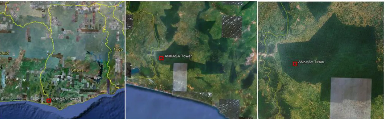
The Ankasa conservation area defines one of the oldest rainforest and the most biodiverse of Ghana. It is the only wet evergreen protected area in practically pristine state with almost 800 vascular plant species and many animal species. Ankasa is relatively uniform in its abiotic landscape features being a relatively undisturbed high forest climax community.

The area is located in southwest Ghana (Fig 1.6) on the border with the Ivory Coast. The protected area covers about 509 km2 [Symonds 2000] and include the Nini-Suhien National

Park and the adjoining Ankasa Resource Reserve (the measurement site). It lies within the

administrative jurisdiction of Jomoro District Assembly and traditionally under the

Paramount Stool of Western Nzema at Beyin. The Nini river is the northern boundary of the

National Park.

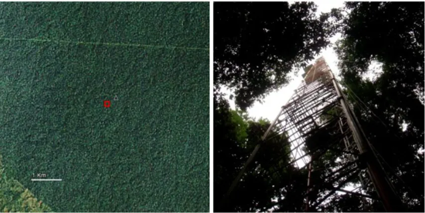
Figure 1.6. Aerial images of the Ankasa forest reserve. The red square indicate the EC measurement tower. The dark green areas are the forest patches. (Images from Google Earth).

The climate is characterised by a distinctive bi-modal rainfall pattern occurring from April to July and September to November. The average annual rainfall is 1700 to 2000 mm. Mean monthly temperatures are typical of tropical lowland forest and range from 24 to 28 °C. Relative humidity is generally high throughout the year, being about 90% during the night falling to 75% in early afternoon.

The soil surface is characterised by rugged, deeply divided terrain in the north and west with flatter swampy ground associated with the Suhien watershed in the east. Its maximum elevation is 150 m at Brasso Hill in the National Park, though most lies below 90 m a.s.l.. The underlying geology consists of three major geological formations. The northern section is based on granites intrusions. The area is at the intermediate erosion stage of maximum slope

19 and is well dissected by an extensive and regular dendritic drainage system. At the south of the granites area there is the area of sediment of clay, hardened and foliated by heat and pressure. The southern most areas are relatively recent deposits.

In general the soils are classified as Forest Oxysols. They are deeply weathered, highly acidic (pH 3.5 to 4.0), disposed to the wind blowing off the Sahara from north, that deposits large quantities of fine soil particles. This annual deposit of clay minerals is likely to play an important role in maintaining forest fertility. The stock of carbon in the mineral soil to a depth of 1 m was measured to be 151 ± 20 Mg C ha-1, a similar value in magnitude to the one of the aboveground biomass being 138-170 Mg C ha-1 including live and dead wood. Surface litter C is roughly 10% (15 ± 9 Mg C ha-1) of the C in the biomass and soil [Chiti et al., 2010]. Recent studies report an average density of 950 plants ha-1, leading to an aboveground biomass of about 270 t ha-1. The LAI (leaf area index) is estimated to be 6 ± 1.01. The distribution of forest-types is largely determined by interacting environmental factors of which climate, geology and soils are the most important. Some of the main species are

Cynometra ananta, Heritiera utilis, Gluema ivorensis, Parkia bicolor, Lophira alata, Strephonema pseudocola, Uapaca guiinensis [Marchesini et al, 2011].

An EC station for the monitoring of GHG and energy fluxes (Fig. 1.6) is operative as part of the CarboAfrica eddy covariance network. The facility, located in the Ankasa Conservation Area includes a 65 m tall steel tower equipped with a system enabling the measurements of fluxes at the top of the structure, air temperature and humidity along a vertical profile and of relevant physical parameters of the forest ecosystem.

A preliminary analysis made in August 2008 indicated a daily uptake of 1.33 ± 0.73 g C m-2 d-1 with the CO2 flux measured above the canopies ranging from a night efflux of 2.3 to a

day-time uptake of -14.8 µmol m-2 s-1. The build-up of the CO2 concentration in the closed canopy

space at night (i.e. CO2 storage) determines an underestimation of the ecosystem respiration

on average by a factor 2 - 2.5 and by a maximum of 4 [Marchesini et al, 2011] demonstrating the importance of storage correction in such environment.