Beta estimation on different trading periods

UNIVERSITY OF CATANIA

Research doctorate courses 31

cycle

Economics, Management and Statistics

Beta Estimation on

Different Trading Periods

Candidate: Alessandra Insana

Supervisor: Prof. Edoardo Otranto

Co-supervisor: Prof. Walter Distaso

Introduction 1

1 Systematic risk and beta estimation 3

Introduction . . . 3

1.1 The Capital Asset Pricing Model . . . 4

1.2 Constant beta estimation . . . 6

1.3 Time-varying beta estimation . . . 8

1.4 High-frequency data and trading period on beta estimation . . . . 10

2 Daily, intraday and overnight betas 13 Introduction . . . 13

2.1 Local least square kernel regression . . . 14

2.2 Kernel . . . 15

2.3 Bandwidth . . . 16

2.3.1 Ruppert rule of thumb . . . 17

2.3.2 Ang and Kristensen . . . 19

2.4 Data and Estimation . . . 21

Conclusion . . . 37

Appendix A . . . 39

3 BAB daily, intraday and overnight 71 Introduction . . . 71

3.1 The BAB factor . . . 72

3.2 Methodology . . . 74

3.3 Daily, intraday and overnight BAB factor . . . 76

3.4 Results . . . 77

Conclusion . . . 84

Appendix B . . . 86

The purpose of this thesis is to investigate on beta estimation considering dif-ferent trading periods. Starting from a literature review, given in the first chapter, we explain the meaning of beta and the different methodologies used for its esti-mation. We find that there is poor literature evidence on the differences between daily, intraday and overnight betas, so we decide to focus on this topic.

In order to understand if beta estimation on different trading periods matter, in the first chapter, we divide the total daily return in intraday and overnight re-turn and evaluate daily, intraday and overnight betas using two different models. Starting by the classical Capital Asset Pricing Model (CAPM), and assuming a constant systematic risk, i.e. a constant beta over time, we estimate our three betas. Subsequently, we consider a nonparametric method for time-varying con-ditional betas, proposed by Ang and Kristensen (2012) and Li and Yang (2011). By using this model we compute time-varying betas in conditional factor models which are conditional on the realized betas. For both these models we estimate daily, intraday and overnight betas considering US stocks traded on the NYSE, AMEX, and NASDAQ markets. Furthermore, we try to understand if there is some relation between the beta parameter and the stock size. Taking into account the differences in pattern between the daily intraday and overnight betas, found in the second chapter, we decide to investigate if it is possible to take advantage of the different behaviors in a trading strategy based on the beta estimation. In particular, we consider the statistical arbitrage strategy, proposed by Frazzini and Pedersen (2014), Betting Against Beta (BAB) and we adapt it constructing three different portfolios ranked and organized by daily, intraday and overnight betas.

Part of this work has been presented at the 4th Conference of the International Society for Nonparametric Statistics (ISNPS 2018).

Systematic risk and beta estimation

Introduction

When we talk about investments we have to talk about risk. Every individual investment is exposed to two types of risk: unsystematic risk and systematic risk. Unsystematic risk, said also residual risk or diversifiable risk, represents the risk related to one security or to a group of specific securities, it is indeed associated to microeconomics factors. This kind of risk can be mitigated through diversi-fication, investing on securities belonging to different sectors. Systematic risk depends on the uncertainty related to the market. Macroeconomic factors, like inflation, change in interest rate, recession and wars, can be considered as sources of systematic risk. This kind of risk cannot be diversified, it can be mitigated by a good asset allocation strategy, and so investing on different financial products (i.e. bonds and stocks). When markets are perfect and frictionless, and we have a well diversified portfolio, the only relevant risk is systematic risk (Elton et al., 2009), that can be evaluated by beta, ’β’.

Beta can be considered as a measure of the systematic risk, it represents the stock’s sensitivity of returns with respect to the changes in the market. A beta less than one implies that the investment will be less volatile than the market. A beta greater than one indicates that the investment’s price will be more volatile than the mar-ket. This suggests that a risk-averse investor will choose to invest on a stock with a low beta. A not risk-averse investor will consider a stock with a beta greater than one. Of course higher risk implies higher profit.

Beta is an unknown coefficient, unobservable to investors. Various evaluation strategies have been proposed in order to obtain a more precise estimator as proxy for its true value. The simplest way is to consider the CAPM and evaluate beta by a classical OLS method, assuming a constant beta on the whole period. This assumption has been criticized because it implies a constant systematic risk over

time, and this is not realistic because systematic risk represents the uncertainty inherent to the market. In order to overcome this problem, and evaluate time-varying beta, several different econometric methods have been proposed. The most popular approaches consider non parametric techniques, different versions of the GARCH model and Kalman filtering procedure.

In the first sections we give a literature review on beta estimation. We present the limits of the CAPM and the different econometric methodologies used for constant and time-varying betas evaluation. Finally we talk about beta estimation through the use of high frequency data, and on different trading periods.

1.1

The Capital Asset Pricing Model

When we talk about beta, the first model that we have to consider is the Cap-ital Asset Pricing Model (CAPM), developed by Sharpe (1964), Lintner (1965) and Mossin (1966), where beta represents the slope from regressing the asset re-turns on market rere-turns. The expected return of a security, E(r), expressed by the classical CAPM is given by:

E(r) = rf+β[E(rM)− rf] , (1.1)

where rf is the return of a risk free investment and rM is the return from the market portfolio. If we denote with R = r− rf and RM= rM− rf the excess return on the security and on the market portfolio, we can write the model as:

E(R) =βE(RM) . (1.2)

Another parameter, which is often used in combination with beta, is the alpha or Jensen index (Jensen, 1968) and it is related with volatility or risk. It can be used to determine how much the realized return of the security differs from the theoretical return determined by the CAPM. Mathematically speaking it is given by:

α = E(r)− rf−β[E(rM)− rf] . (1.3) It provides a relationship between risk and return (technically called ’security mar-ket line’ SML). Its value describes the performance of an investment in relation with its benchmark. In an efficient market we expect that this value is equal to zero. Having negative values for alpha means that we have a security’s under-performance, on the other hand having a positive alpha means that our security outperform its benchmark index.

The CAPM gives a way to measure the relationship between expected return and risk. It is one of the most used models for the portfolio performance anal-ysis. As in all mathematical models also in the CAPM there are some implicit assumptions, as reported in Hull (2012):

1. “Investors care only about the expected return and the standard deviation of return of their portfolio”;

2. “The returns from investments are correlated with each other only because of their correlation with the market portfolio”;

3. “Investors focus on returns over just one period and the length of this period is the same for all investors”;

4. “Investors can borrow and lend at the same risk-free rate”; 5. Tax does not influence investment decisions;

6. “All investors make the same estimates of expected returns, standard devia-tions of returns, and correladevia-tions between returns”.

To test the validity of the CAPM, many empirical studies have been conducted, considering time-series and cross-sectional regressions. First studies support the CAPM (Fama et al., 1969; Blume, 1970), but subsequently, some empirical re-searches put some questions on the explanatory power of market betas for explain-ing the cross-section of expected returns (Basu, 1977, 1983; Roll, 1977; Banz, 1981; Stattman, 1980; Rosenberg et al., 1985; Bhandari, 1988; Fama and French, 1992). It is important to mention that verify the accuracy of CAPM could be dif-ficult, because if the value used as proxy for the market is inefficient, the resulting beta estimates are less accurate (Roll, 1977; Ross, 1977; Roll and Ross, 1994). The poor empirical results obtained, probably due to the very restrictive and unre-alistic assumptions of the CAPM, brought to a long review debate, in which many authors tried to develop and extend some of the crucial problems, in order to give a more realistic model (for reviews of the CAPM literature see Campbell (2000); Fama and French (2004); Jagannathan et al. (2010a,b); Subrahmanyam (2010); Goyal (2012)).

The most discussed assumptions are the first one, for which investors look only at the first two moments of return distribution, and the third one, in which the model assumes a constant risk over time. The first hypothesis implies that returns are normally distributed, but this is not true for many assets that have skewness and excess kurtosis. This is supported by empirical results, in which it has been shown that the corresponding third and fourth moment (skewness and kurtosis) of asset distribution are very different from those of the normal distribution (Kraus and Litzenberger, 1976; Harvey and Siddique, 2000; Hwang and Satchell, 1999; Fang and Lai, 1997).

Probably one of the most criticized assumptions of the CAPM, is related to consider the risk associated with an asset constant over time. Indeed, in reality, investment horizon consists of many periods, and many studies showed empirical

evidence for time-varying risk premia of financial assets (Shiller et al., 1984; Let-tau and Ludvigson, 2001b). To overcome this problem there are two ways. The first one considers a multiple source of systematic risk, by intertemporal models developed by Merton (1973) and then extended by the three-factor model of Fama and French (1993) and multifactor models.

For example Fama and French (1993), in order to explain the expected returns of an investment, introduce in the CAPM other sources of systematic risk related to size and book to market through the following three factor model:

E(r)− rf = +βM[E(rM)− rf] +βSE(SMB) +βhE(HML) , (1.4)

where SMB (Small Minus Big) is the difference between the returns on portfolios of small and large stocks, HML (High Minus Low) is the difference between portfolios of high and low book to market value stocks.

The second methodology, used to add time-varying systematic risk factors, im-plies the evaluation of conditional time-varying models (Jagannathan and Wang, 1996; Lettau and Ludvigson, 2001a). Considering conditional variances and co-variances (Bodurtha and Mark, 1991), conditional factor models and conditional CAPM are a good way to include the time-varying systematic risk factors. From literature it seems that the use of a conditional version of the CAPM could better explain the systematic risk (Jagannathan and Wang, 1996; Lettau and Ludvigson, 2001a).

By the conditional CAPM, we have the following relationship:

E[ri,t− rf ,t|Ft−1 ] = E [βi,t|Ft−1] E [ rM,t− rf ,t|Ft−1 ] , (1.5)

here all the parameters are estimated at time t, they are conditional toFt−1, that represents the information set at time t− 1. This equation can be written as:

E [Ri,t+1|Ft] = E [βi,t+1|Ft] E [RM,t+1|Ft] , (1.6) where the conditional beta can be evaluated as:

E [βi,t+1|Ft] =

cov [Ri,t+1, RM,t+1|Ft] var [RM,t+1|Ft]

.

1.2

Constant beta estimation

The most adopted approach for beta estimation, assumes the systematic risk as constant, and evaluates it by an ordinary least squares (OLS) method. Consid-ering a bivariate time series (Ri, RMi)ni=1of excess returns of a security and excess market returns, the empirical formulation of the CAPM (1.1) can be written as:

where α is expected to be zero, εi are the error terms i.i.d, and the systematic risk beta, is the estimated slope of the linear regression of Ri on RMi. It can be evaluated considering the sample covariance between the excess returns of a security and excess market returns divided by the sample variance of the excess market returns:

ˆ

β = cov(Ri, RMi) var(RMi)

. (1.8)

If the covariance with the return of the market is zero we will have beta equal to zero, so a risk free asset, otherwise, if the covariance is equal to the market variance, we will have beta equal to one.

An equivalent beta formula is given by: ˆ

β =ρ σ

σM

,

whereσ andσM are the standard deviation of the security returns and of the mar-ket returns,ρ represents their correlation.

Evaluating beta by a simple OLS method is not efficient, because the market is complex and volatile. For example, OLS is not suitable for estimating beta coeffi-cient in the cases of normal distribution, tail or other distributions, that cannot be explained successfully by the model. Furthermore the existence of outlier or ex-treme data can create a problem of efficiency for the OLS regression model (Jiang, 2011; Shalit and Yitzhaki, 2002; Martin and Simin, 2003; Tofallis, 2008). To elim-inate standard parametric model inefficiency, robust regression techniques have been developed (Genton and Ronchetti, 2008; Alp and Bilir, 2015). For exam-ple Sharpe (1971) considers the least absolute deviations (or the L1-estimator) for beta estimation. Chan and Lakonishok (1992) use quantile regression, linear com-binations of regression quantiles, and trimmed regression quantiles. Martin and Simin (2003) propose to evaluate beta by means of redescending M-estimators.

The across time instability given by OLS standard beta estimation, can be overcome considering different strategies. For Blume (1970) and Levy (1971), it is possible increase precision of beta, grouping stocks into portfolios and com-pute the beta, for each portfolio, in time series regression. Other authors (Baesel, 1974; Altman et al., 1974; Blume, 1975; Roenfeldt et al., 1978) assert that a more stable evaluation can be given considering a longer estimate period. Furthermore, has been proposed the use of autoregressive adjustment methods (Blume, 1975; Vasicek, 1973). The Blume (1975) autoregressive adjustment method, try to cap-ture the tendency of the standard betas to converge towards the value of unity over time. Considering how much the historical betas are different from their average value, Blume regresses betas from one historical period on beta from a prior pe-riod and then uses this regression to adjust betas for the forecast pepe-riod. Instead,

Vasicek (1973) develops a Bayesian estimation technique, considering the accu-racy of the historical betas. In particular, he modifies the past betas in relation to the average beta, taking into account the value of the beta sampling error. When this error is higher, there could be an higher difference from the average beta. To betas with a larger sampling error will be assigned a lower weight. Respect to the standard evaluation, these two adjustment techniques led to a more accurate fore-cast for beta (Klemkosky and Martin, 1975; Luoma et al., 1996; Murray, 1995; Hawawini et al., 1985; Sarker, 2013). As shown by Cloete et al. (2002) the use of robust estimators with the Vasicek’s technique, generates a new class of estimators that perform better respect to the traditional.

1.3

Time-varying beta estimation

Market risk premia changes over time, consequently stock betas will vary over time, implying a change in the stock’s price (Bollerslev et al., 1988; Lettau and Ludvigson, 2001b). The betas used within the CAPM are calculated on a set period-by-period basis, ignoring its continuous evolution. Assuming a constant beta the CAPM does not describe the cross-section of average returns on equities and the market, considered to explain dynamics in volatility (Bos and Newbold, 1984; Collins et al., 1987; Brooks et al., 1992; Choudhry, 2002, 2005; Adrian and Franzoni, 2009).

In order to estimate time-varying betas it is possible adopt more sophisticate strategies. The most used methods make assumptions about the dynamics of be-tas (parametric and non-parametric approaches, considering rolling regression, Kalman filters) or make assumptions about the conditional covariance matrix of returns (GARCH models).

Applying a parametric approach, we can model beta as a function of state vari-able (Shanken, 1990) or firm characteristics (Jagannathan and Wang, 1996; Lettau and Ludvigson, 2001a). Shanken (1990) assumes a linear relation between beta and some state variables, and estimates the parameters of this function in a con-ditional CAPM time-series regression. Jagannathan and Wang (1996) and Lettau and Ludvigson (2001a) represent the variation of the conditional distribution of returns as a function of lagged state variables. They model the covariance be-tween the market returns and portfolio returns defining affine functions of these variables. With this approach beta can be estimated by a multi-factor model, in which the additional factors are given by the relations between the market return and the state variables. There is also a non parametric version of this methodology (Ferreira et al., 2011).

Kalman filters give a direct estimate of time varying betas. Betas are cal-culated from an initial set of priors, producing a series of conditional betas,

as-suming standard stochastic processes such as random walk, autoregressive, mean reverting and switching models (Black et al., 1992; Wells, 1994; Faff et al., 2000; Brooks et al., 2002; Hillier, 2002; Gao and Yao, 2004; Ebner and Neumann, 2005; Mergner and Bulla, 2008).

The GARCH models use the conditional variance information to construct the conditional beta series. Generally, for time-conditional moments models is con-sidered an autoregressive moving average relation. The first who introduced the Autoregressive Conditional Heteroscedasticity (ARCH) model was Engle (1982). Subsequently, in order to parametrize the conditional mean and the conditional covariance of financial time series, Bollerslev (1986) introduces the Generalized ARCH (GARCH). The Multivariate-GARCH (M-GARCH) model, first proposed by Bollerslev (1990), evaluates the beta time-series indirectly, considering the es-timates of the time-varying conditional covariance of security and market returns and the time-varying conditional variance of market returns. The GARCH ap-proach for time-varying beta has been considered in various studies (Bollerslev et al., 1988; Engel and Rodrigues, 1989; Braun et al., 1995; Giannopoulos, 1995; McClain et al., 1996; Bodurtha and Mark, 1991; Brooks et al., 1998; Lie et al., 2000; Brooks et al., 2002; Li, 2003; Mergner and Bulla, 2008; Darolles et al., 2018). Instead of the multivariate-GARCH models it is possible consider a new class of multivariate models called Dynamic Conditional Correlation (DCC) mod-els proposed by Engle (2002). As said by the author these estimators “have the flexibility of univariate GARCH but not the complexity of conventional multivari-ate GARCH”. In recent papers Engle (2016) and Bali et al. (2016) consider this model for beta estimation.

The last methodology for the estimation of time-varying betas assumes that betas vary smoothly over time. Starting from the Fama and MacBeth (1973) work, it is possible to consider a rolling window ordinary least square estima-tion. Considering this approach we do not have a parametrization problem, but we have to select the window length. Within the family of rolling least squares es-timators, we can include the nonparametric time-varying betas estimator (Robin-son, 1989) and nonparametric time-varying conditional betas (Esteban and Orbe-Mandaluniz, 2010; Li and Yang, 2011; Ang and Kristensen, 2012).

Many different papers evaluate the various approaches for time-varying betas, discussed above. The most compared are the GARCH-based estimators and the Kalman filter approaches. By the results obtained it seems that the last methodol-ogy performs better in terms of forecasting ability (Faff et al., 2000; Mergner and Bulla, 2008; Adrian and Franzoni, 2009; Choudhry and Wu, 2008; Nieto et al., 2014; Bali et al., 2016).

1.4

High-frequency data and trading period on beta

estimation

During the last few years there has been an explosion in the amount of fi-nancial high frequency data. This led to the improvement and the development of new techniques and models for the evaluation of financial parameters, both in time-series than in cross-sectional dimensions.

Using higher frequency data, on simple autoregressive time series models, allows a more accurate beta estimation and forecasting (Barndorff-Nielsen and Shephard, 2004; Andersen et al., 2005, 2006). Furthermore, systematic risk estimation with daily-frequency data, can give a good relationship between betas and the cross-section of expected stock returns. For example Bali et al. (2016), considering dynamic conditional beta at daily frequency, find that results are efficient in ex-plaining the cross-section of daily stock returns, confuting the previous empirical tests for which the CAPM fails to describe the cross-section of stock returns (Fama and French, 1992).

The use of high-frequency data allows also the development of new estima-tors. Starting from techniques used for realized volatility (Foster and Nelson, 1994; Andersen and Bollerslev, 1998), it is possible forecast and model a new estimator for beta, the ’realized betas’ (Barndorff-Nielsen and Shephard, 2004; Andersen et al., 2005, 2006; Patton and Verardo, 2012). These new beta estimates are time-varying and are defined as the ratio between the realized covariance of stock and market and the realized market variance. They can be considered as a non-parametric estimator of underlying beta.

One of the most relevant aspects, when we talk about high frequency data, is the sampling frequency. Indeed, using low-frequency data, could determine im-precise and noisy estimates for beta (Andersen et al., 2006), but conducting the analysis to a very high frequency induces distortion on estimate, because intra-day returns are corrupted by the market microstructure noise, due to the market friction. In order to overcome these problems, it is possible consider different approaches like adjustments by including filtering (Ebens et al., 1999; Andersen et al., 2001; Bandi and Russell, 2005), subsampling (Andersen et al., 2011), cor-rection for overnight price changes (Hansen and Lunde, 2004), considering kernel estimators (Hansen and Lunde, 2004; Barndorff-Nielsen et al., 2011).

Most of the papers, using high-frequency data, do not take into account the non trading effect in their estimation, indeed they employ just intraday values. For example, Ryu (2011) finds that the realized beta, computed using only the intraday returns, provides a good estimation of underlying beta that could outperform the constant beta.

improve the forecast accuracy of models based on daily returns (Taylor and Xu, 1997; Koopman et al., 2005; Pong et al., 2004; Liu and Maheu, 2009; Fuertes and Olmo, 2013). Although, ignoring completely the overnight period, considering only the intraday returns, could be an error, because of course non-trading periods influence the following trading hours. The computation of financial measures, including the overnight return, could change significantly, from those that exclude that values.

Different authors, analyzing intraday and overnight price returns, show a dif-ference in return patterns (Tsai et al., 2012; Branch and Ma, 2012, 2006; Cooper et al., 2008; Berkman et al., 2009; Wang et al., 2009). Many of them find that day-time returns and overnight returns tend to be anti-correlated. For example, Tsai et al. (2012) investigate on the correlation between the three components on the Taiwan stock market, and compare their results with others markets as the New York Stock Exchange (NYSE) and the National Association of Securities Dealers Automated Quotation (NASDAQ). They find a negative cross correlation between the sign of daytime returns and the sign of overnight returns. Also Branch and Ma (2006) and Wang et al. (2009) show that daytime returns and overnight returns are significantly negatively correlated. In particular, Wang et al. (2009) studying the statistical distribution and correlation between total return, overnight return, and daytime return, on 2215 stocks in New York Stock Exchange, find an higher mean value for daytime returns respect to overnight. In opposition, Gallo (2001), shows that daytime returns and overnight returns are not significantly negatively correlated, furthermore, Kelly and Clark (2011) and Cooper et al. (2008) suggest that stock returns are higher overnight than intraday.

Analyzing the momentum returns Bogousslavsky (2016) and also Polk et al. (2018), find that it increases overnight. Indeed their empirical studies show that intraday, momentum returns do not exhibit any clear pattern except at the end of the day, when returns tend to be negative. This is probably related to overnight liquidity risk.

Obviously, periodic market closures impact also on stock price volatility. Volatil-ity of returns during trading periods is found to be higher, than those during non trading periods (French and Roll, 1986; Lockwood and Linn, 1990; G¨uner and

¨

Onder, 2002). Also Linton and Wu (2017), in a recent paper, analyzing second moments, and so volatility, they find that intraday is higher than overnight. Al-though between 2009 to 2012 they note higher values for overnight volatility, due probably to the European sovereign debt crisis. Furthermore, the ratio between overnight and intraday volatility is increasing over part of the last 20 years.

Many approaches have been considered in realized volatility literature, most of them ignore completely the non trading effect and scale upward the value ob-tained, in this way the evaluation includes an entire 24-hour day (Koopman et al., 2005; Martens, 2002). Hansen and Lunde (2005) derive optimal weights for the

overnight return and the sum of intraday returns. Other authors (Bollerslev et al., 2009; Pooter et al., 2008; Martens, 2002; Blair et al., 2010) estimate the overnight return subtracting the day’s close value from the next day’s open, and add this squared return as one of the factors in the sum of intraday returns. Andersen et al. (2011) model the overnight returns as discontinuous movements.

Few authors put their attention on beta estimation considering different trading periods. Liu (2003) evaluates the relationship between a security’s systematic risk, considering high-frequency data for overnight and intraday returns. He computes the security beta as a weighted average of its intraday beta and overnight beta, the weight is the variance ratio between the intraday market index return and the overnight market index return. Considering different trading periods for beta esti-mation, Todorov and Bollerslev (2010) suggest a pricing framework in which they evaluate three separate market betas: a continuous beta for the ’smooth’ intraday co-movements with the market, and two ’rough’ betas associated with intraday price discontinuities, or jumps, during the trading hours, and the overnight close-to-open return. They found that the average of the two rough betas is higher than the continuous beta.

Daily, intraday and overnight betas

Introduction

As we have seen in the first chapter, there are many papers about the financial meaning of beta and the different methodologies used for its estimation, on the other hand few studies investigate on the value of intraday and overnight betas.

Since we want to understand whether evaluating systematic risk, i.e. beta, on different trading periods could lead to different results and if there are some dif-ferences in patterns between the daily, intraday and overnight betas, we divide the total daily return into intraday and overnight return. In order to do that, in this chapter, we focus our attention on two models, the first one uses constant beta and the other one allows time-varying beta.

The first evaluation is obtained starting from the classical CAPM applying a sim-ple OLS method. As we said in the first chapter this is not the best choice for beta estimation because this model assumes a constant systematic risk over time and furthermore because there are obvious inefficiency problems using a standard parametric model.

For the time-varying betas we consider the conditional CAPM, and we solve it us-ing a non parametric method through a standard weighted regression in which the kernel is around time. This procedure for conditional betas has been proposed by Robinson (1989) and then by Ang and Kristensen (2012) and Li and Yang (2011). We choice this approach because it can be quite simple and flexible from a computational point of view, these are fundamental features considering the va-riety of comparisons that we want to do and the big amount of data. Of course the choice of the kernel and the bandwidth represents a crucial point for efficient results. In particular, in order to obtain more accurate values, we decide to use a Gaussian kernel and three different bandwidths for our estimations. As first band-width we consider the simple Silverman’s rule (Silverman, 1986), then we adopt

the optimal bandwidth evaluated by Ang and Kristensen (2012) and finally we derive an optimal bandwidth adapting the Ruppert et al. (1995)’s rule of thumb. Daily, intraday and overnight betas are estimated considering US stocks values traded on the NYSE, AMEX, and NASDAQ markets. The data have been taken from the Center for Research in Security Prices (CRSP). As benchmark for the market index we first consider the same daily value for all the trading periods, subsequently we use our intraday and overnight weighted index. In order to un-derstand if there is some relationship between beta and the size, we evaluate our betas stock by stock but also grouping them into ten portfolios sorted month by month by market capitalization.

In the first sections of this chapter we present the conditional CAPM and the methodology used for beta evaluation, focusing on the kernel and bandwidth se-lection. In the last section we explain our procedure and show our results.

2.1

Local least square kernel regression

We evaluate our time-varying beta starting by the conditional CAPM, where the excess returns of a generic stock, at discrete time points t = 1,··· ,n, respect to the excess market returns, are given by:

Rt=αt+βtRMt+ωtzt, (2.1)

αt and βt are the conditional alphas and betas, zt is the error term and ωt is the conditional variance of errors.

Considering the filtration Ft =F (Rj, RM j,αj,βj : j≤ t) the error term have to satisfies E [ ztFt ] = 0 , E [ ztz′tFt ] = 1 , (2.2)

these assumptions can be viewed as a generalization of the classical OLS condi-tions, they state that errors and factor are orthogonal.

Under the orthogonality condition (2.2), there is a conditional relation between parameter and observation, Ang and Kristensen (2012), define the realization of alphas and betas that generated data as:

[αt,βt]′=Λ−1t E [

XtRt′|Ft ]

,

where Xt = (1, RMt)′ andΛt = E [XtXt′|Ft] is the conditional second moment of the regressors.

As other authors have done (Robinson, 1989; Li and Yang, 2011; Ang and Kristensen, 2012; Esteban and Orbe-Mandaluniz, 2010), in order to estimate the

model (2.1) we assume that the sequences of αt andβt, vary smoothly over time and lie on unknown functions of the time index:

αt =α(t/n) ∈ C2[0, 1] and βt=β(t/n) ∈ C2[0, 1] .

This assumption makes αt andβt dependent on the sample size n. We map each observation labelled by t = 1, 2,··· ,n, into an interval between 0 and 1 through the transformation t/n. We do not impose a functional form but we use local in-formation to estimate the two quantities, for this reason the method can be viewed as a non-parametric method.

Given the observations of excess returns and excess market returns at t = 1, 2,··· ,n, it is possible to derive an estimate of the functions α(τ) and β(τ), for a generic asset, at any normalized time pointτ ∈ (0,1). This is done using a local least square kernel regression:

[ ˆ α(τ), ˆβ(τ) ]′ = arg min (α,β) n

∑

K(·) is a kernel function and h the bandwidth.

Solving the equation (2.3) we can obtain the optimal estimators running, for each asset, a series of kernel-weighted ordinary least square (OLS) regressions

[ ˆ α(τ), ˆβ(τ) ]_′ = [ n

∑

∑

The use of a kernel function gives the possibility to estimate conditional alphas and betas at any time, using all the data efficiently. Obviously, the most relevant aspect of the implementation of this method is the selection of the kernel shape and the bandwidth h.

2.2

Kernel

Using a kernel function we assign different weights to the observations. These weights depend on how close the observations are to the point τ. The most fre-quently used kernel functions are the uniform function

K(τ) = {

1

2, for|τ| ≤ 1 0 , for|τ| > 1

and the Epanechnikov kernel function K(τ) = { 3 4(1−τ 2_{) , for|τ| ≤ 1} 0 , for|τ| > 1

In the first case, all the observations have the same weights. In the second one, the observations closer to the estimation pointτ have an higher weight compared to those farther from it. This implies that weights decline with the increase of the time lag. Although many authors like Li and Yang (2011), Andersen et al. (2006) and Lewellen and Nagel (2006) use one-sided and uniform kernel, following Ang and Kristensen (2012), we consider for our estimates, a Gaussian density

K(τ) =√1 2πexp ( −τ2 2 ) .

The main problem that can occur using a two-sided symmetric kernel is an excess of bias at the beginning and at the end of the sample. There are many techniques that could be used to avoid this problem, such as locally linear kernel estimator or boundary kernels. The simplest methodology, used also by Ang and Kristensen (2012), is to delete the first and the last year of the conditional betas estimated. In particular in our estimation we evaluate our beta on all the time period and delete the results related to the first and last year. For this reason for the single stocks analysis we consider only that with more than three years of observations.

2.3

Bandwidth

As pointed by many authors, the bandwidth selection is perhaps the most cru-cial choice for this method. A small h tends to correspond a small bias in betas and alphas, at the same time a large h involves a small variance in the estimates, for these reasons we need estimate it optimally. The most popular techniques for the bandwidth selection are the cross-validation method (Rudemo, 1982; Bow-man, 1984; Robinson, 1989) and the plug-in method (Sheather and Jones, 1991; Ruppert et al., 1995). The first one is completely data driven, on the other hand the second requires to choose some unknown parameters, in order to estimate the optimal window size. We decide to implement our procedure considering three different bandwidths: the Silverman’s rule (Silverman, 1986) for a data driven bandwidth and two plug-in methods considering the Ang and Kristensen (2012) methodology and a the modified Ruppert’s rule of thumb (Ruppert et al., 1995).

Applying the Silverman’s rule (Silverman, 1986) we evaluate the bandwidth for each stock as:

Clearly this first choice is the simplest one from a computational point of view, it depends just on the number of observations that we are considering. Conversely, it is not optimal since it considers just the time vector, ignoring other data.

The other two optimal global bandwidths can be obtained minimizing the con-ditional Integrated Mean Square Error (MISE), given by:

∫ ₁ 0 [ bias ( ˆ β(τ) )]2 + var ( ˆ β(τ) ) dτ.

Bias and variance of our beta are:

bias ( ˆ βt ) =1 2µ2β (2) t h2, var ( ˆ βt ) =ν₀[n hΛFF t]−1σt2, where: µ2= ∫ u2K(t)dt = 1 andν0= ∫

K(t)2dt = 1/2√π= 0.2821 for a Gaussian kernel.

ΛFF t =ΛFF(t/n) is the conditional variance of our factor and σt2=σ2(t/n) is the conditional variance of residuals. β_t(2)=β(t/n)(2) whereβ(·)(2) denotes the second order derivative ofβ(t/n).

The optimal bandwidth can be written as:

hopt= [ ν0 ∫1 0 ΛFF(τ)−1σ2(τ)dτ n∫₀1β(τ)(2)2_dτ ]1/5 . (2.5)

In order to apply this formula we have to derive the conditional variance of the factor and the conditional variance of residuals which depend on unknown pa-rameters. First we evaluate them adapting the Ruppert’s rule of thumb procedure (Ruppert et al., 1995) and then we use the Ang and Kristensen (2012) bandwidth selection.

2.3.1

Ruppert rule of thumb

Ruppert et al. (1995) in their paper give some methodologies for bandwidth selection in local least square regression. We emphasize that we need to adjust their method to our case since in our work the kernel is around time and this means that we are dealing with a different model. In particular, we modify the rule of thumb procedure, in which, assuming conditional variance and conditional variance of residual as constants, they estimate the unknown parameters used in the bandwidth formula by a blocked quartic fit. They divide data into blocks and for each block they evaluate the parameters. The optimal block, used in the for-mula, is chosen by the Mallows’s Cp(Mallows, 1973).

ConsideringΛ_{FF t}= var(RM) andσt2=σ2as constants and denoting B = ∫1 0β (2) τ 2 dτ, equation (2.5) can be written as:

h =

[

ν0σ2

n var(RM) B ]1/5

where σ2 and B are unknowns, so we need to estimate them by the following procedure.

1. Considering our n observations we divide them inχjblocks for j = 1,··· ,N, where the maximum number is given by:

Nmax= max{min(⌊n/20⌋,N∗), 1} (2.6)

we select N∗= 5, like in the Ruppert’s paper.

2. We assume βt = b0+ b1(t/n) + b2(t/n)2+ b3(t/n)3+ b4(t/n)4, a polyno-mial of order 4, and we estimate these coefficients applying a parametric least square method for each block j by the following equation:

Rt =α+ ( b0+ b1(t/n) + b2(t/n)2+ b3(t/n)3+ b4(t/n)4 ) RM t+εt (2.7) t =⌊( j − 1)n/N⌋ + 1,··· ,⌊ jn/N⌋ and j = 1,··· ,N .

For each block j we obtain: ˆ

βQj t = ˆb0 j+ ˆb1 j(t/n) + ˆb2 j(t/n)

2_{+ ˆb}

3 j(t/n)3+ ˆb4 j(t/n)4. (2.8)

3. Once we get ˆβ we can estimate ˆBQas ˆ BQ(N) =1 n n

∑

∑

∑

∑

∑

∑

it can be written as ˆ σ2 Q(N) = 1 (n− 5N) jn/N

∑

∑

5. In order to derive the optimal block ˆN, following Mallows (1973), from the

set{1,2,··· ,Nmax}, we consider the one that minimizes

Cp(N) =

RSS(N)(n− 5Nmax)

RSS(Nmax) − (n − 10N) ,

(2.14)

where RSS(N) =∑_t∈N(Rt− ˆα− ˆβ(t/n)RM t)2is the residual sum of squares of a blocked quartic N-block-OLS.

6. Considering the previous estimates, we can now compute the modified Rup-pert rule-of-thumb bandwidth ˆhRas

ˆhR= [ ν0σˆ_Q2( ˆN) n var(RM) ˆBQ( ˆN) ]1/5 . (2.15)

2.3.2

Ang and Kristensen

Ang and Kristensen (2012) use for their conditional beta estimation a global plug-in bandwidth. They start from the methodology presented by Ruppert et al. (1995), but they take into account also the time-varying correlation between beta and the factor. Their procedure for the bandwidth selection involves two steps. In the first step they evaluate a preliminary bandwidth, considering for the unknown parameters of equation (2.5) parametric estimates. In the second step they use this first bandwidth for conditional beta, conditional variance and conditional standard errors computation that will be used in the bandwidth formula (2.5). We show below in detail their procedure.

1. From equation (2.5) we can considerΛ_{FF t}= var(RM) andσt2=σ2as con-stants and write B =∫₀1β_τ(2)2dτ, so h can be written as:

h =

[

ν0σ2

n var(RM) B ]1/5

In order to estimateσ2and B, we consider, for t = 1,··· ,n

βt= b0+ b1(t/n) + b2(t/n)2+ b3(t/n)3+ b4(t/n)4+ b5(t/n)5+ b6(t/n)6 a polynomial of order 6, and evaluate the coefficients applying parametric least square on this equation:

Rt=α+βtRMt+εt t = 1,··· ,n (2.16) obtaining ˆ βt= ˆb0+ ˆb1(t/n) + ˆb2(t/n)2+ ˆb3(t/n)3+ ˆb4(t/n)4+ ˆb5(t/n)5+ ˆb6(t/n)6. (2.17) We evaluate ˆB as ˆ B =1 n n

∑

where ˆβ_t(2)represents the second derivative given by: ˆ β(2) t = 2ˆb2+ 6ˆb3(t/n) + 12ˆb4(t/n)2+ 20ˆb5(t/n)3+ 30ˆb6(t/n)4. (2.19) We compute ˆσ2as ˆ σ2₌ 1 n n

∑

Considering the previous estimates, we now can evaluate the first step band-width h1as: h1= [ ν0σˆ2 var(RM) ˆB n ]1/5 . (2.21)

2. Once obtained h1we estimate the variance components and ˆβ(τ). ˆ ΛFF(τ) = ∑ n t=1Kh1(t/n−τ) [RMt− ˆµF(t/n)] 2 ∑n t=1Kh1(t/n−τ) where ˆ µ(τ) = ∑ n t=1Kh1(t/n−τ)RMt ∑n t=1Kh1(t/n−τ)

is an approximation of the conditional mean.

The conditional variance of residual,σ2(τ), can be computed as: ˆ σ2_{(τ) =} ∑t=1n Kh1(t/n−τ) ˆε 2 t ∑n t=1Kh1(t/n−τ)

where ˆεt= ˆε(t/n) = Rt− ˆα(t/n)− ˆβ(t/n)RMt. The numerator of equation (2.5) can be written as:

ˆ V =ν0 1 n n

∑

The denominator of (2.5) is given by:

ˆ B =1 n n

∑

where ˆβ(τ)(2) is the second derivative, with respect toτ, of the kernel esti-mator: ˆ β(τ) = ∑ n t=1K¯h1 ∑ n t=1K¯h1RMtRt− ∑ n t=1K¯h1RMt ∑ n t=1K¯h1Rt ∑n t=1K¯h1 ∑ n t=1K¯h1R 2 Mt− [∑nt=1K¯h1RMt] 2 . where ¯Kh1= Kh1(t/n−τ).

Considering the previous estimates we can evaluate the bandwidth as

ˆh_AK= [ _ˆ V n ˆB ]1/5 . (2.22)

2.4

Data and Estimation

In our empirical analysis we evaluate US stock betas, traded on the NYSE, AMEX, and NASDAQ markets. We compute daily, intraday and overnight betas by an unconditional and a conditional CAPM. As benchmark for the market, we first use, for all the trading periods, the same daily excess market return, provided by French’s data library1. After that we assign a market index for daily intraday and overnight period. The conditional betas are computed considering the three different bandwidths exposed in the previous paragraph. We conduct our analy-sis evaluating betas stocks by stocks and then, for a more complete analyanaly-sis, we aggregate them in ten portfolios sorted by market capitalization.

The data are taken from the Center for Research in Security Prices (CRSP)2. The original data set covers the period from December 31, 1925 to December 30, 2016. Since daily open prices are not available between July 1962 and June 1992, we decided to consider just the series from June 15, 1992 to December 30, 2016.

1_{http://mba.tuck.dartmouth.edu/pages/faculty/ken.french/data_}

library.html

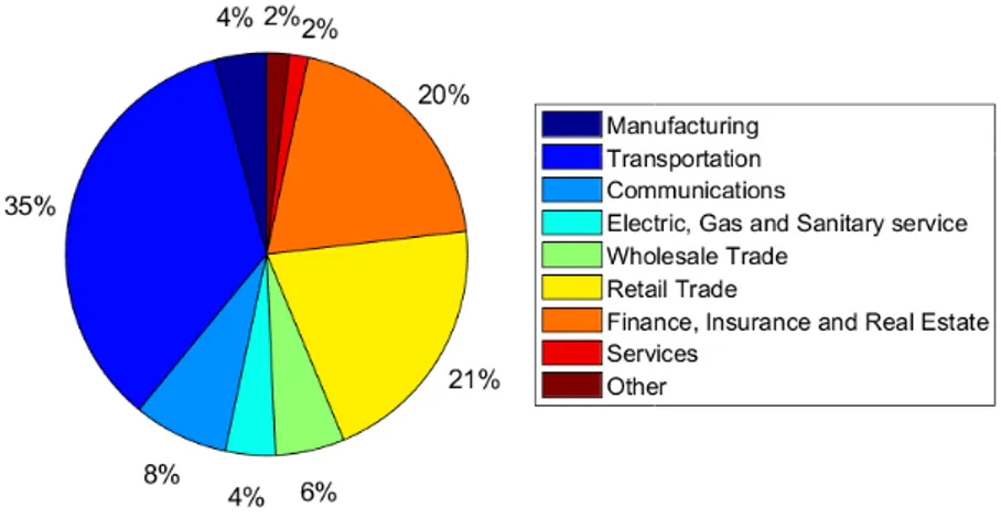
We have 15125 stocks to analyze, as shown in Figure 2.1, the stocks belong to different industry areas and are divided according to the Standard Industrial Clas-sification (SIC) code associated to each stock. The most significant percentage of stocks, 35%, belong to transportation, communications, electric, gas and sanitary service sectors, the 21% belong to retail trade and 20% to finance, insurance and real estate sectors. In the case of the stock by stock analysis we exclude from the data set all the stocks with less of three years of observations, i.e. with less of 765 business days, obtaining 10849 stocks to analyze. We delete these stocks because, as we said previously, the estimator for time-varying beta could give biased results on the tails and for this reason we need to delete the first and last year estimate betas from the analysis.

Figure 2.1:Percentage of CRSP stock, from June 16, 1992 to December 30, 2016 divided by the

Standard Industrial Classification (SIC) code.

In order to evaluate the daily, intraday and overnight returns, we adjust open and closing price for dividends and splits, by the cumulative adjustment factor, provided by the CRSP data set (CFACPR). The total return or daily return (close-to-close) are calculated on the close price of the previous trading day and the close price of the subsequent trading day:

rd_t = p close t

p_t−1close− 1 .

It can be decomposed, in daytime or intraday (open-to-close) and overnight (close-to-open) return: rid_t = p close t popen_t − 1, r ov t = popen_t p_t−1close− 1 .

The intraday returns are calculated over the trading hours, from current day opening to closing. The overnight returns are computed considering the variation

of the price from the previous trading day closure to current trading day opening. Following Bogousslavsky (2016), for the excess returns computation we subtract the daily risk-free rate, representing the daily treasury bill returns and obtained from Kenneth French’s database, from our daily and overnight returns. This must be done because intraday returns transactions are settled at the end of the day thus the risk-free rate should not be earned (Heston et al., 2010).

In order to compare the results and before we compute any beta we adjust our dataset so as to keep for each stock only those days in which we have daily, intraday and overnight returns.

Market Index Correlation

MRFF _MRd _MRid _MRov MRFF 1

MRd 0.9997 1

MRid _{0.8515 0.8517 1} MRov _{0.5468 0.5470 0.0274 1}

Table 2.1: Correlations between the Fama

and French daily market return (MRFF)

with our daily (MRd_{), intraday (MR}id_{) and}

overnight (MRov_{) weighted market index.}

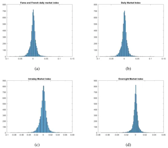
Market Index MRFF _MRd _MRid _MRov Mean 0.0004 0.0004 0.0002 0.0002 Std. dev. 0.0114 0.0115 0.0096 0.0060 Variance 0.0001 0.0001 0.0001 0.0000 Skewness -0.1339 -0.1303 -0.1513 -0.6397 Kurtosis 11.1109 11.1048 11.2023 16.8949

Table 2.2: Some statistics of daily Fama and

French’s market index (MRFF) and the daily

(MRd), intraday (MRid) and overnight (MRov)

weighted market index computed. Index series are from June 16, 1992 to December 30, 2016.

For the purpose of having a more precise comparison, we decide to evaluate betas considering also an intraday and overnight market benchmark. We think that by a dimensionality point of view, it could be more correct to have a market value for each trading period. Unfortunately, we do not have the value of the open price of the market, in addition we are considering stocks belonging to three different markets. Therefore, in order to have a daily, intraday and overnight market index we construct a weighted index for each trading period, considering all the stocks in the series, from June 16, 1992 to December 30, 2016. Our market index is given by the following formulas:

MRd_t =∑iwi, tr d i, t ∑iwi, t , MR_tid =∑iwi, tr id i, t ∑iwi, t , MR_tov= ∑iwi, tr ov i, t ∑iwi, t , wi, t = pclose_{i, t−1}si, t−1 are the weights for each stock i at time t given by the mar-ket capitalization. We take the values of the number of shares outstanding, s, from CRSP database and adjust them considering a cumulative adjustment fac-tor (CFACSHR). We also evaluated the weights for intraday period, considering open price and number of shares outstanding at the time t, but since we did not

find relevant differences, we decide to consider the same weight for each trading period.

We find that the Fama and French index correlates very highly with our daily and intraday indices, also intraday and overnight market indices seem to be corre-lated (Table 2.1). The mean and standard deviation of our daily index is similar to Fama and French (Table 2.2). All the four series have a negative skew, this means that the left tail is longer and the mass of the distribution is concentrated on the right. This behaviour is more evident for overnight market index. Furthermore the series exhibit a positive excess kurtosis, and so a leptokurtic distribution. These results are also shown in the histograms of Figure 2.7 in Appendix A.

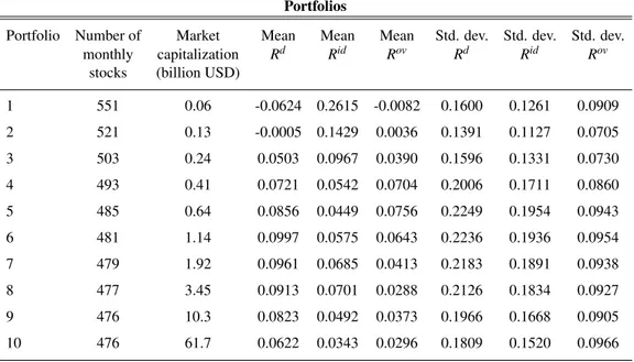
Portfolios

Portfolio Number of Market Mean Mean Mean Std. dev. Std. dev. Std. dev. monthly capitalization Rd _Rid _Rov _Rd _Rid _Rov

stocks (billion USD)

1 551 0.06 -0.0624 0.2615 -0.0082 0.1600 0.1261 0.0909 2 521 0.13 -0.0005 0.1429 0.0036 0.1391 0.1127 0.0705 3 503 0.24 0.0503 0.0967 0.0390 0.1596 0.1331 0.0730 4 493 0.41 0.0721 0.0542 0.0704 0.2006 0.1711 0.0860 5 485 0.64 0.0856 0.0449 0.0756 0.2249 0.1954 0.0943 6 481 1.14 0.0997 0.0575 0.0643 0.2236 0.1936 0.0954 7 479 1.92 0.0961 0.0685 0.0413 0.2183 0.1891 0.0938 8 477 3.45 0.0913 0.0701 0.0288 0.2126 0.1834 0.0927 9 476 10.3 0.0823 0.0492 0.0373 0.1966 0.1668 0.0905 10 476 61.7 0.0622 0.0343 0.0296 0.1809 0.1520 0.0966

Table 2.3: Monthly average of the number of stock and market capitalization of each portfolio.

Annualized mean and standard deviation of the daily intraday and overnight excess returns of our

portfolios, are computed multiplying for 252 and√252, respectively.

For a more complete and simple analysis we aggregate our stocks in portfo-lios. As we said in the first chapter, this could allows a more precise beta es-timation (Blume, 1970; Levy, 1971). In order to do this, on the last day of the month, we evaluate the market capitalization for each stock traded and then we sort our stocks in ascending order and divide them in ten portfolios. Portfolio 1 contains stocks with lower market capitalization, each month on average a total of 60 milliards USD. Instead, portfolio 10 has stocks with higher market capital-ization, each month on average 61 billions USD. The series are from July 1, 1992 to December 30, 2016 and so in each portfolio we have 6170 trading days. As

we show in Table 2.3 in each decile we have on average 500 stocks traded each month. Furthermore evaluating the daily, intraday and overnight returns, in excess of the risk free rate (annualized, i.e. multiplied by 252), we find that almost all portfolios have a greater daily excess return and a lower overnight return. Also evaluating the annualized standard deviation, multiplying for √252, we note an higher volatility for daily returns. Looking at the table and at the cumulative re-turns represented in Figure 2.9 Appendix A, we note an higher value for intraday return in the first and second portfolio.

We start analyzing the values of the constant betas, for all the single stocks, obtained applying the simple OLS model. We observe that, considering the daily Fama and French market index for all the trading periods, on 10 849 stocks, 9 586 have an intraday beta greater than overnight, so, only 1 263 have the opposite rela-tionship. If instead we compute betas with a daily intraday and overnight market index we obtain 6 122 stocks with an intraday beta greater than overnight and so 4 727 with an overnight larger than intraday. This means that to consider or not an equal market index, for all the trading periods, changes significantly the value of intraday and overnight betas. The main statistics, computed considering the values obtained by each stock, are in Table 2.4. With a variable market index, our three betas have the same means, although the distribution is different (Figure 2.8 Appendix A), furthermore we have a greater variation for overnight betas.

Market Index Daily intraday and overnight

Fama and French Market Index

βd _βid _βov _βd _βid _βov

Mean 0.7663 0.5654 0.2013 0.7659 0.7301 0.7217

Std. dev. 0.4663 0.3742 0.1745 0.4655 0.5028 0.4673

Table 2.4:Mean and standard deviation of the betas across all the stocks. Betas are computed, for

each stock, by OLS considering first Fama and French market index and then daily, intraday and overnight market index.

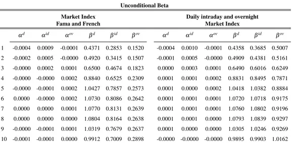
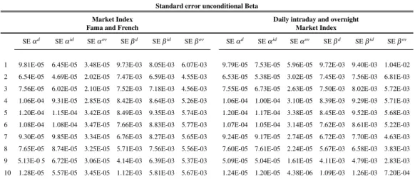
Aggregating our stocks in ten portfolios by market capitalization, we note that the values of betas on all periods are increasing by size (Table 2.5). Furthermore, as in the case of the single stocks, we have higher values for intraday and overnight betas, if we consider the specific trading market benchmark. Using a weighted in-dex the values of daily and intraday betas are very similar, instead the overnight values remain lower. These results are better shown by Figure 2.2, in which we add the 95% confidence interval by the error bars. Looking at these results and to the value of standard error for alphas and betas (Table 2.6) we can say that our estimate is sufficiently precise. Although, as we have seen in the first chapter, to

assume a constant beta is not the best choice, because systematic risk varies with time.

Unconditional Beta

Market Index Daily intraday and overnight

Fama and French Market Index

αd _αid _αov _βd _βid _βov _αd _αid _αov _βd _βid _βov 1 -0.0004 0.0009 -0.0001 0.4371 0.2853 0.1520 -0.0004 0.0010 -0.0001 0.4358 0.3685 0.5007 2 -0.0002 0.0005 -0.0000 0.4920 0.3415 0.1507 -0.0001 0.0005 -0.0000 0.4909 0.4381 0.5161 3 -0.0000 0.0002 0.0001 0.6500 0.4674 0.1823 0.0000 0.0003 0.0001 0.6490 0.6016 0.6249 4 -0.0000 -0.0000 0.0002 0.8840 0.6525 0.2309 0.0001 0.0001 0.0002 0.8831 0.8495 0.7871 5 -0.0000 -0.0001 0.0002 1.0427 0.7857 0.2573 0.0001 0.0000 0.0002 1.0418 1.0382 0.8884 6 0.0000 -0.0000 0.0002 1.0730 0.8086 0.2642 0.0001 0.0001 0.0001 1.0720 1.0718 0.9175 7 0.0000 0.0000 0.0001 1.0770 0.8131 0.2639 0.0001 0.0001 0.0001 1.0760 1.0802 0.9196 8 0.0000 0.0000 0.0000 1.0804 0.8164 0.2638 0.0001 0.0001 0.0000 1.0793 1.0839 0.9297 9 -0.0000 -0.0001 0.0001 1.0319 0.7679 0.2637 0.0001 0.0000 0.0000 1.0305 1.0246 0.9269 10 -0.0001 -0.0001 0.0000 0.9912 0.7009 0.2898 -0.0000 -0.0000 -0.0000 0.9895 0.9903 1.0162

Table 2.5: Unconditional alpha and beta on 10 Portfolios. Portfolios are divided and sorted

con-sidering the market capitalization at the end of each month. Alphas and betas are evaluated in each portfolio considering the same daily Fama and French market index and also with a daily intraday and overnight market index.

(a) (b)

Figure 2.2: Unconditional beta values on the 10 portfolios. Betas are evaluated considering the

Fama and French market index (a) and a daily intraday and overnight market index (b). We plot also the 95% confidence interval by the error bars.

Standard error unconditional Beta

Market Index Daily intraday and overnight

Fama and French Market Index

SEαd _SEαid _SEαov _SEβd _SEβid _SEβov _SEαd _SEαid _SEαov _SEβd _SEβid _SEβov

1 9.81E-05 6.45E-05 3.48E-05 9.73E-03 8.05E-03 6.07E-03 9.79E-05 7.53E-05 5.96E-05 9.72E-03 9.40E-03 1.04E-02 2 6.54E-05 4.69E-05 2.02E-05 7.47E-03 6.59E-03 4.55E-03 6.53E-05 5.38E-05 3.02E-05 7.45E-03 7.56E-03 6.81E-03 3 7.56E-05 6.02E-05 2.10E-05 7.52E-03 7.18E-03 4.56E-03 7.55E-05 6.73E-05 2.63E-05 7.50E-03 8.02E-03 5.72E-03 4 1.06E-04 9.31E-05 2.85E-05 8.42E-03 8.64E-03 5.26E-03 1.06E-04 1.00E-04 3.10E-05 8.39E-03 9.29E-03 5.71E-03 5 1.20E-04 1.15E-04 3.42E-05 8.49E-03 9.35E-03 5.74E-03 1.20E-04 1.17E-04 3.38E-05 8.45E-03 9.52E-03 5.68E-03 6 1.08E-04 1.08E-04 3.47E-05 7.66E-03 8.83E-03 5.77E-03 1.07E-04 1.05E-04 3.14E-05 7.62E-03 8.61E-03 5.22E-03 7 9.30E-05 9.85E-05 3.34E-05 6.76E-03 8.27E-03 5.65E-03 9.24E-05 9.17E-05 2.74E-05 6.72E-03 7.70E-03 4.63E-03 8 7.65E-05 8.74E-05 3.25E-05 5.71E-03 7.56E-03 5.56E-03 7.60E-05 7.61E-05 2.24E-05 5.67E-03 6.58E-03 3.83E-03 9 5.13E-0 5 6.72E-05 3.06E-05 4.14E-03 6.39E-03 5.37E-03 5.09E-05 5.04E-05 1.61E-05 4.11E-03 4.79E-03 2.83E-03 10 1.28E-05 5.57E-05 3.45E-05 1.12E-03 5.81E-03 5.67E-03 1.24E-05 1.20E-05 4.38E-06 1.09E-03 1.26E-03 7.20E-04

Table 2.6: Standard error for the unconditional beta estimate on the 10 Portfolios. Portfolios are

divided and sorted considering the market capitalization at the end of each month. Alpha and beta are evaluate in each portfolio considering the same daily Fama and French market index and also with a daily intraday and overnight market index.

We begin now to analyze the results obtained applying, stock by stock, the conditional CAPM. As for the constant beta analysis we consider the same daily Fama and French market index and our daily, intraday and overnight weighted index. Furthermore, as we said, we use three different bandwidths: Silverman (1986), a modified Ruppert et al. (1995) and Ang and Kristensen (2012). Look-ing at Figure 2.3, in which we represent the daily, intraday and overnight mean of beta across the stocks in the period, it is obvious the time-varying nature of betas and their difference behaviors. In particular we observe that daily, intraday and overnight betas, obtained by considering a daily intraday and overnight mar-ket index, are very similar until the 2000, then overnight is always lower respect the daily and intraday that have very similar values in all the following time pe-riod. Furthermore, we can notice that all three beta values are increasing from November 2004.

(a) (b)

(c) (d)

(e) (f)

Figure 2.3: Mean of conditional betas day by day. We evaluate conditional betas stock by stock

and plot the mean of betas for each day. Beta evaluation are given considering the Silverman

(hS), the modified Ruppert (hR) and the Ang and Kristensen (hAK) bandwidths. On the left betas

computed considering the Fama and French daily market index; on the right betas computed with weighted market index for each trading period.

Using the first two bandwidths we obtain very similar results and there could be a little undershooting in our estimate, so the Ang and Kristensen bandwidth seems to be the better choice. Similar results are evident also analyzing single stocks, in which sometimes we have an overlapping between the Silverman and modified Ruppert bandwidths (Figure 2.10 Appendix A), and looking at the mean of the bandwidths, across all stocks (Table 2.7). The values of these two band-widths are similar and larger respect than of Ang and Kristensen.

Bandwidth

Market Index Daily intraday and overnight

Fama and French Market Index

hS hdR hidR hovR hdAK hidAK hAKov hdR hidR hRov hdAK hidAK hovAK

mean 0.0664 0.0782 0.0797 0.0860 0.0471 0.0479 0.0537 0.0782 0.0792 0.0792 0.0470 0.0475 0.0481

std. dev. 0.0083 0.0277 0.0279 0.0294 0.0203 0.0202 0.0224 0.0279 0.0276 0.0290 0.0202 0.0200 0.0204

Table 2.7:Mean and standard deviation across the bandwidth of all the stocks. We consider three

bandwidths: the constant bandwidth of Silverman (1986) (hs) equal for all the trading periods; the

modified Ruppert et al. (1995) bandwidth (hR) and that of Ang and Kristensen (2012)(hAK). The

last two are different for each portfolio and each trading period, furthermore we evaluate them also with the Fama and French market index and daily, intraday and overnight market index.

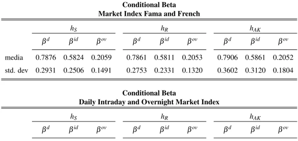
Conditional Beta Market Index Fama and French

hS hR hAK

βd _βid _βov _βd _βid _βov _βd _βid _βov

media 0.7876 0.5824 0.2059 0.7861 0.5811 0.2053 0.7906 0.5861 0.2052 std. dev 0.2931 0.2506 0.1491 0.2753 0.2331 0.1320 0.3602 0.3120 0.1804

Conditional Beta

Daily Intraday and Overnight Market Index

hS hR hAK

βd _βid _βov _βd _βid _βov _βd _βid _βov

media 0.7876 0.7499 0.7322 0.7860 0.7486 0.7316 0.7904 0.7525 0.7324 std. dev 0.2927 0.3105 0.3484 0.2750 0.2914 0.3220 0.3598 0.3814 0.4357

Table 2.8:Mean of conditional beta across the stocks. Time-varying betas are evaluated stock by

stock considering the same daily Fama and French market index and daily intraday and overnight market index.

On average our three time-varying betas have similar values to the uncon-ditional betas (Table 2.8), but different distributions (Figure 2.12 2.11 2.11 Ap-pendix A). Also in this case, we find higher values if we consider a daily, intraday

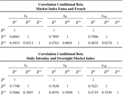
and overnight weighted index as proxy for the market, specially for overnight be-tas. Furthermore, with this approach, we obtain an higher correlation between intraday and overnight betas independently by the bandwidth choice (Table 2.9).

Correlation Conditional Beta Market Index Fama and French

hS hR hAK

βd _βid _βov _βd _βid _βov _βd _βid _βov

βd _{1 1 1}

βid _{0.8062 1 0.7895 1 0.7966 1}

βov _{0.4915 0.0513 1 0.4762 0.0691 1 0.4678 0.0270 1}

Correlation Conditional Beta Daily Intraday and Overnight Market Index

hS hR hAK

βd _βid _βov _βd _βid _βov _βd _βid _βov

βd _{1 1 1}

βid _{0.7790 1 0.7650 1 0.7621 1}

βov _{0.5066 0.3897 1 0.4976 0.3896 1 0.4719 0.3550 1}

Table 2.9: Correlation of conditional beta across the stocks. We evaluate time-varying betas

stock by stock considering the same daily Fama and French market index and daily intraday and overnight market index. Then for each stock we compute the correlation between the three betas, obtained the values for all the stocks we consider the mean across all.

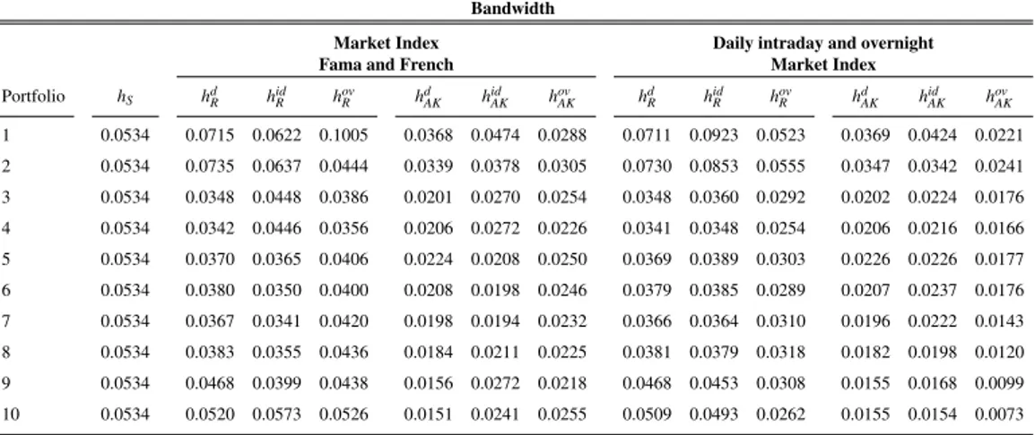
Aggregating our stocks in ten portfolios, sorted by size, and observing the three different bandwidth values, we find that, as for the single stocks case, the bandwidths of Ang and Kristensen (2012) are smaller implying more variability in the betas, instead the Silverman (1986) and the modified Ruppert et al. (1995) bandwidths are very similar (Table 2.10). Considering the same market index or a daily, intraday and overnight give us similar results. As before, the best choice for the bandwidth is the Ang and Kristensen (2012) bandwidth because other two give some under smoothing on betas.

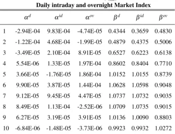
For these reasons, for conditional betas on portfolios, we decide to show just results obtained considering the daily, intraday and overnight market index and the Ang and Kristensen (2012) bandwidth, other cases are in Appendix A. Looking at Table 2.11, displaying for each portfolio the means of alphas and betas across all the period, we note that the values are very similar to the OLS estimates. Indeed, also in this case, beta increases by size and for first and last portfolio overnight beta is greater than intraday. The different trends of our three betas can be

ob-Bandwidth

Market Index Daily intraday and overnight

Fama and French Market Index

Portfolio hS hdR hidR hovR hdAK hidAK hovAK hdR hidR hRov hdAK hidAK hovAK 1 0.0534 0.0715 0.0622 0.1005 0.0368 0.0474 0.0288 0.0711 0.0923 0.0523 0.0369 0.0424 0.0221 2 0.0534 0.0735 0.0637 0.0444 0.0339 0.0378 0.0305 0.0730 0.0853 0.0555 0.0347 0.0342 0.0241 3 0.0534 0.0348 0.0448 0.0386 0.0201 0.0270 0.0254 0.0348 0.0360 0.0292 0.0202 0.0224 0.0176 4 0.0534 0.0342 0.0446 0.0356 0.0206 0.0272 0.0226 0.0341 0.0348 0.0254 0.0206 0.0216 0.0166 5 0.0534 0.0370 0.0365 0.0406 0.0224 0.0208 0.0250 0.0369 0.0389 0.0303 0.0226 0.0226 0.0177 6 0.0534 0.0380 0.0350 0.0400 0.0208 0.0198 0.0246 0.0379 0.0385 0.0289 0.0207 0.0237 0.0176 7 0.0534 0.0367 0.0341 0.0420 0.0198 0.0194 0.0232 0.0366 0.0364 0.0310 0.0196 0.0222 0.0143 8 0.0534 0.0383 0.0355 0.0436 0.0184 0.0211 0.0225 0.0381 0.0379 0.0318 0.0182 0.0198 0.0120 9 0.0534 0.0468 0.0399 0.0438 0.0156 0.0272 0.0218 0.0468 0.0453 0.0308 0.0155 0.0168 0.0099 10 0.0534 0.0520 0.0573 0.0526 0.0151 0.0241 0.0255 0.0509 0.0493 0.0262 0.0155 0.0154 0.0073

Table 2.10:Bandwidth on 10 Portfolios. Portfolios are divided and sorted considering the market

capitalization at the end of each month. We consider three bandwidths: the constant bandwidth

of Silverman (1986) (hs) equal for all the portfolios and for all the trading periods; the modified

Ruppert et al. (1995) bandwidth (hR) and that of Ang and Kristensen (2012)(hAK). The last two

are different for each portfolio and each trading period, furthermore we evaluate them also with the Fama and French market index and daily, intraday and overnight market index.

served in Figure 2.4 (in Figure 2.19, Figure 2.20, Figure 2.21 in Appendix A, we show same results adding, in dashed lines, the 95% confidence bands), from portfolio 3 to portfolio 8 we have a greater variability, furthermore the daily and intraday betas have similar behaviors while overnight remain lower. In particular looking at these portfolios we note an increasing value for beta between August 2002 and September 2006. Looking to lower cap and higher cap portfolios we can see lower variations between betas, but higher values for portfolio 10, in which all the three betas varying around one.

Conditional Beta (hAK)

Daily intraday and overnight Market Index αd _αid _αov _βd _βid _βov

1 -2.94E-04 9.83E-04 -4.74E-05 0.4344 0.3659 0.4830 2 -1.22E-04 4.68E-04 -1.99E-05 0.4879 0.4375 0.5006 3 -3.49E-05 2.10E-04 8.91E-05 0.6527 0.6223 0.6138 4 5.54E-06 1.33E-05 1.97E-04 0.8602 0.8404 0.7710 5 3.66E-05 -1.76E-05 1.86E-04 1.0152 1.0155 0.8739 6 9.90E-05 3.87E-05 1.44E-04 1.0628 1.0598 0.9048 7 9.12E-05 9.45E-05 4.47E-05 1.0737 1.0732 0.9035 8 8.49E-05 1.13E-04 -2.52E-06 1.0709 1.0735 0.9015 9 6.27E-05 3.19E-05 3.91E-05 1.0136 1.0090 0.8803 10 -6.84E-06 -1.48E-05 -3.73E-06 0.9923 0.9932 1.0272

Table 2.11:Mean of conditional alpha and beta on 10 Portfolios. Portfolios are divided and sorted

considering the market capitalization at the end of each month. Time-varying alpha and beta are evaluated in each portfolio considering a daily intraday and overnight market index. Results are from June 30, 1993 to December 31, 2015.

(a) (b)

Figure 2.4: Conditional betas on portfolios 1-2 between June 30, 1993 to December 31, 2015.

Portfolios are divided and sorted considering the market capitalization at the end of each month. Time-varying betas are evaluated in each portfolio considering a daily intraday and overnight market index and the Ang and Kristensen bantwidth.

(a) (b)

(c) (d)

(e) (f)

Figure 2.4: Conditional betas on portfolios 3-8 between June 30, 1993 to December 31, 2015.

Portfolios are divided and sorted considering the market capitalization at the end of each month. Time-varying betas are evaluated in each portfolio considering a daily intraday and overnight market index and the Ang and Kristensen bantwidth.