TABLE OF CONTENTS
1 Introduction ... 5
2 LAMMPS code ... 7
3 Interatomic potentials ... 9
4 Details of calculations ... 13
5 Results ... 14
5.1 Linear thermal expansion ... 14
5.2 Enthalpy and specific heat ... 15
5.3 Thermal conductivity ... 16
5.4 Melting temperature ... 19
6 Conclusions ... 19
1 INTRODUCTION
Nowadays, the nuclear fuels employed in reactors are uranium dioxide and MOX. The planned deployment of a new generation of fast reactors will require the use of MOX fuel. The foreseen concentration of plutonium dioxide ranges up to 30 mol% (Sen09). Plutonium recycling from spent nuclear fuel increases the economic performance while reducing plutonium stockpiles. In the long term, breeding fast reactors will overcome the limitation in uranium resources improving the sustainability of nuclear energy. The use of plutonium dioxide in nuclear fuel must comply with the safety requirements adopted in all the stages of nuclear fuel cycle. With regard to this topic, a sound knowledge of the thermophysical properties of PuO2 is certainly
relevant (Kat15). Toxicity, high radiation level, and behaviour at high temperature are all factors that make the measurement of PuO2 thermophysical properties complex
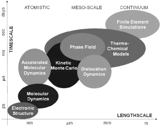
(Bal17). The use of numerical approaches could be helpful in overcoming these obstacles. Beside this aspect, these methodologies give insight into the physical phenomena occurring in the fuel matrix. In this frame, classical molecular dynamics (MD) occupies an important research area between the density functional theory (DFT) and the coarse grained mesoscale models (NEA15). The most important methodologies considered in a Multi-scale approach to the simulation of nuclear fuel behaviour are presented in Fig. 1.1.
Thanks to its capabilities, MD gives the opportunity to study relevant phenomena for the description of thermo-mechanical behaviour in nuclear fuel such as:
thermal-mechanical properties; radiation damage;
fission gas bubbles formation/resolution; dislocation loops formation/motion; grain boundary motion;
fuel densification.
The relevance of this methodology for the development and improvement of existing fuel performance codes is acknowledged. For example, one of the key parameters of fission gas release models is the resolution coefficient. MD methodology could make the determination of this quantity achievable (Uff15).
Interatomic potentials play a central role in MD. These functions describe the force field acting on the elements of the system (atoms/ions). They are analytical functions whose parameters are usually tuned to predict with good accuracy the available experimental data (e.g., lattice parameter and thermal expansion, bulk modulus). The definition of these parameters could also be based on ab initio calculations.
In the course of a Molecular Dynamics simulation the classical equations of motion are solved at each time step. Atoms basically interact with each other through van der Waals attractive forces, short-range repulsive forces, and electrostatic forces. If they are covalently bonded, strong forces hold them together as stable chemical groups. From this microscopic information a series of macroscopic observables like pressure, temperature, heat capacity, stress tensor etc. are determined using statistical mechanics through time averages. The validity of this approach is based on the hypothesis that the system is ergodic. In these systems time averages are equivalent to ensemble averages. MD simulations are performed under specific ensembles. The micro-canonical ensemble is a fundamental ensemble. It is characterized by constant number of particles N, constant volume V, and constant total energy E (NVE). Other ensembles are the canonical or NVT ensemble and the isothermal-isobaric or NPT ensemble (feasible by introducing a coupling to appropriate ‘thermostats’ and ‘barostats’) (Bin04).
Following the activity started in the frame of PAR2016 within the Accordo di Programma between ENEA and the Italian Ministry of Economic Development (MiSE), this report presents the results of Molecular Dynamics (MD) calculations performed using four interatomic potentials for the simulation of PuO2. These
potentials are employed for the calculation of some relevant thermophysical properties: thermal expansion, specific heat, thermal conductivity, and melting temperature. Predictions are compared with the experimental measurements published in the literature. The MD calculations presented in this report were performed by means of the LAMMPS code (Large-Scale Atomic/Molecular Massively Parallel Simulator) (Pli95). This activity was conducted within the frame of project B3-LP1-A.2.2 (PAR2017).
These results were presented at the International Conference Nuclear Energy for New Europe, Portorož, Slovenia, September 10–13, 2018 (paper 705).
In the following sections a brief description of the LAMMPS code and the interatomic potentials applied in simulations is given. The details of calculations and results are presented and discussed in the concluding sections.
2 LAMMPS CODE
The review of MD calculations published in the literature confirmed that LAMMPS (Pli95) is one of the most used codes in the analysis and simulation of MOX fuel (Cal17). This code offers the capabilities required for the simulation of MOX and its constituents: UO2 and PuO2. In addition, the code is freely-available. For these
reasons, it was decided to employ LAMMPS for the activity proposed in the current piano annuale di realizzazione of AdP (PAR2017).
LAMMPS is a classical molecular dynamics code capable of modelling an ensemble of particles in a liquid, solid, or gaseous state. The user can model atomic, polymeric, biological, metallic, granular, and coarse-grained systems. LAMMPS integrates the Newton's equations of motion for collections of atoms, molecules, or macroscopic particles that interact via short- or long-range forces with an ample set of initial and boundary conditions. The code uses lists of neighbors to keep track of nearby particles. This approach improves the efficiency of calculations. These lists are constructed under the condition that the local density of particles never becomes too large when repulsive forces are present.
The code runs on single-processor machines, but it is designed for parallel computing on any parallel machines with a C++ compiler and supporting the message passing interface (MPI). LAMMPS is an open-source code whose distribution is ruled by the GNU General Public License. The code was originally developed within the projects managed by the US Department of Energy (DOE) such as CRADA (Cooperative Research and Development Agreement), LDRD, ASCI, and Genomes-to-Life. The core group of LAMMPS developers is now at the Sandia National Laboratories.
Some features of the code are briefly listed below. Some of these options are discussed in more detail in the following two sections.
Particles and model types
atoms;
coarse-grained particles (e.g. bead-spring polymers); united-atom polymers or organic molecules;
metals;
granular materials;
coarse-grained mesoscale models;
finite-size spherical and ellipsoidal particles;
point dipole particles;
rigid collections of particles; hybrid combinations of these.
Force fields
pairwise potentials: Lennard-Jones, Buckingham, Morse, Born-Mayer- Huggins, Yukawa, soft, class 2 (COMPASS), hydrogen bond, tabulated;
charged pairwise potentials: Coulombic, point-dipole;
many-body potentials: EAM, Finnis/Sinclair EAM, modified EAM (MEAM), embedded ion method (EIM), EDIP, ADP, Stillinger-Weber, Tersoff, REBO, AIREBO, ReaxFF, COMB, SNAP, Streitz-Mintmire, 3-body polymorphic;
long-range interactions for charge, point-dipoles, and LJ dispersion: Ewald, Wolf, PPPM;
polarization models: QEq, core/shell model, Drude dipole model;
charge equilibration: QEq via dynamic, point, shielded, Slater methods; coarse-grained potentials: DPD, GayBerne, REsquared, colloidal, DLVO; mesoscopic potentials: granular, Peridynamics, SPH;
electron force field: eFF, AWPMD;
bond potentials: harmonic, FENE, Morse, nonlinear, class 2, quartic (breakable);
angle potentials: harmonic, CHARMM, cosine, cosine/squared, cosine/periodic, class 2 (COMPASS);
dihedral potentials: harmonic, CHARMM, multi-harmonic, helix, class 2 (COMPASS), OPLS;
improper potentials: harmonic, cvff, umbrella, class 2 (COMPASS); polymer potentials: all-atom, united-atom, bead-spring, breakable; water potentials: TIP3P, TIP4P, SPC;
implicit solvent potentials: hydrodynamic lubrication, Debye;
force-field compatibility with common CHARMM, AMBER, DREIDING, OPLS, GROMACS, COMPASS options;
access to KIM archive of potentials via pair kim;
hybrid potentials: multiple pair, bond, angle, dihedral, improper potentials can be used in one simulation;
overlaid potentials: superposition of multiple pair potentials.
Atom creation
read in atom coordinates from files;
create atoms on one or more lattices (e.g., grain boundaries); delete geometric or logical groups of atoms (e.g. voids); replicate existing atoms multiple times;
Ensembles, constraints, and boundary conditions
2d or 3d systems;
constant NVE, NVT, NPT, NPH, Parinello/Rahman integrators; thermostatting options for groups and geometric regions of atoms; pressure control via Nose/Hoover or Berendsen barostatting in 1 to 3
dimensions;
simulation box deformation (tensile and shear); rigid body constraints;
Monte Carlo bond breaking, formation, swapping; atom/molecule insertion and deletion;
walls of various kinds;
non-equilibrium molecular dynamics (NEMD);
variety of additional boundary conditions and constraints.
3 INTERATOMIC POTENTIALS
The review presented in (Cal17) showed that few types of interatomic potentials are employed in MD research on oxide nuclear fuels. A brief description of the interatomic potentials discussed in the literature is given in this section. The correlations presented here are complete and applicable only when all their coefficients are set. Coefficients are usually determined by fitting the experimental data of specific properties such as the lattice parameter, bulk modulus, elastic properties, etc. Therefore, potentials used in MD are semi-empirical. As presented in (Ari05), the interatomic potential shown in Eq. 1 is the partial ionic model of the Born-Mayer-Huggins pair potential (BMH). The first term accounts for the long-range Coulomb potential, the following two terms correspond to the short-range interactions due to the Pauli’s repulsion principle and the van der Waals forces, respectively. In this correlation the f0 coefficient is an empirical parameter used to adjust the model.
Parameters zi and zj are the effective electronic charges. They are consistent with the
level of ionicity assumed in the atomic bonds. Finally, the term rij is the distance
between atom i and atom j. As aforementioned, the parameters a, b, c are set by fitting the experimental data and are specific of the type of atoms/ions included in the system under consideration. In the case of MOX, the elements to be considered are: oxygen, uranium, and plutonium. If the fuel is non-stoichiometric, the different valence of ions should be properly considered.
6 0 2
exp
)
(
)
(
ij j i j i ij j i j i ij j i ij ijr
c
c
b
b
r
a
a
b
b
f
r
e
z
z
r
U
(1)The Born–Mayer–Huggins potential used in the fully ionic model is presented in Eq. 2. The second term represents the Pauli’s repulsion principle; the third term the short-range van der Waals interactions. In the Coulomb term, full electronic charges should be considered (Ari05). The meaning of symbols is coincident with the
description given above where Aij, ij, and Cij are the empirical coefficients of the
interacting pair of ions.
6 2
exp
)
(
ij ij ij ij ij ij j i ij ijr
C
r
A
r
e
z
z
r
U
(2)The second and third terms in Eq. 2 is also called Buckingham potential. Eq. 1 and Eq. 2 are similar forms of a BMH interatomic potential. Covalent bonds are usually modelled by means of an interatomic potential called Morse potential (Eq. 3). This potential accounts for the covalent interaction between anions and cations. The rij*
parameter is the anion–cation bond length. Dij and ij are the depth and the shape of
the Morse potential.
exp
2
(
)
2
exp
(
)
)
(
* * ij ij ij ij ij ij ij ij ijr
D
r
r
r
r
U
(3)The potential developed by Cooper et al. (Coo14) is presented in Equations 4, 5, 6, and 7. As shown in Eq. 4, this potential is composed of one term expressing the force field acting on the pairs of atoms included in the system. The second term accounts for the presence of many-body interactions. The pair potential is composed of three terms: Coulomb, Buckingham, and Morse and accounts for short- and long-range interactions (Eq. 5). The analytical expression of the first two terms is presented in Eq. 6. An effective ionicity is used for the definition of the ionic charges assumed in calculations. The term expressing the covalent part of atomic bonds (M) is consistent
with the correlation presented in Eq. 3.
2 1
)
(
)
(
2
1
j ij j ij ir
G
r
E
(4))
(
)
(
)
(
)
(
( ) ( ) ( ) ij M ij B ij C ijr
r
r
r
(5) 6 0 ) ( ) (exp
4
)
(
)
(
ij ij ij ij B ij Cr
C
r
A
r
z
z
r
r
(6)The many-body perturbation is proportional to the square root of the sum of terms whose analytical expression is given Eq. 7. G is the constant of proportionality. This
effect is a function of the inverse of the 8-th power of the distance between ions where n is an empirical coefficient. A short range cut-off at 1.5 angstrom is applied
to avoid that these forces could overcome the short-range pair repulsion (Coo14).
8
)
(
ij ijr
n
r
(7)Table 3.1 lists the coefficients of the PuO2 interatomic potentials employed in the
calculations. For the sake of simplicity, these potentials were named: Uchida (Uch14), Yamada (Yam00), Arima (Ari05), and Cooper (Coo14). With regard to the Cooper potential, in addition to the coefficients presented in Tab. 3.1, the values of
G and n applied in calculations were 1.231 eV.Å1.5 and 1456.773 Å5, respectively.
In this case, the results were obtained by means of the numerical file available in (Coo18). The potential by Arima does not consider the covalent term. This potential is entirely modelled by means of the BMH shown in Eq. 2. The Yamada and Arima interatomic potentials were developed in the domain 300-2000 K while the other interatomic potentials were defined in a more ample temperature region up to 3000 K (Cooper) and 3100 K (Uchida).
Potential Uchida Yamada Arima Cooper
Ionicity ζ 0.565 0.6 0.675 0.5552 Aij (eV) O-O 603615.4650 2345.89 978.713 830.283 Pu-Pu 0.0 32606.66 2.80458e+14 18600 Pu-O 5616.1017 5329.81 57424.90 377.395 ij (Å) O-O 0.178285 0.32 0.3320 0.3529 Pu-Pu 0.2 0.16 0.0650 0.2637 Pu-O 0.251699 0.24 0.1985 0.3793 Cij (eV.Å 6) O-O 93.4977 4.1457 17.3500 3.8843 Pu-Pu 0.0 0.0 0.0 0.0 Pu-O 0.01000 0.0 0.0 0.0 Dij (eV) Pu-O 0.187245 0.56411 0.0 0.7019 ij (Å-1) Pu-O 2. 1.56 0.0 1.980 rij* (Å) Pu-O 2.37 2.339 0.0 2.346
Pu-O, Pu-Pu, O-O interatomic potentials are shown in Figs. 3.1-3.3. The values of potentials take into account short-range and long-range interactions. It is worth reminding that the largest contribution comes from the Coulomb potential. With regard to the Cooper potential, the data shown in these figures does not account for the many-body perturbation.
1 3 5 7 9 -30 -20 -10 0 10 20 30 P u -O in te ra to m ic p o te n tia l ( e V ) Distance (Å) Uchida Yamada Arima Cooper
Figure 3.1: Pu-O interactions in applied potentials.
1,0 1,5 2,0 2,5 3,0 0 200 400 600 800 1000 P u-P u in te ra to m ic p ot en tia l ( eV ) Distance (Å) Uchida Yamada Arima Cooper
1,0 1,5 2,0 2,5 3,0 0 200 400 600 800 1000 O -O in te ra to m ic p ot en tia l ( eV ) Distance (Å) Uchida Yamada Arima Cooper
Figure 3.3: O-O interactions in applied potentials.
4 DETAILS OF CALCULATIONS
This report presents the results of MD calculations focused on some relevant PuO2
thermophysical properties: lattice parameter, thermal expansion, enthalpy, specific heat, thermal conductivity, and melting temperature. The temperature of the system lies in the interval 300-3200 K. Values of the lattice parameter and enthalpy were sampled during the measurement period. The results showed here are the averages of these sets of data. The linear thermal expansion was determined from the lattice parameter results. The specific heat was estimated by means of the numerical derivative of enthalpy. The thermal conductivity of PuO2 was evaluated by means of
the Green-Kubo correlation (Gre54). In this approach the thermal conductivity is calculated from the time-integral of the auto-correlation function of heat currents. The Green-Kubo correlation is presented in Eq. 8.
0 2(
)
(
0
)
3
1
J
t
J
dt
V
T
k
k
B (8)In this correlation KB is the Boltzmann’s constant, V is the simulated cell volume, T is
the absolute temperature, and J(t) is the heat flux occurring at the time t. The details of reference calculations are given in Tab. 4.1.
The equilibration period follows an initial calculation to determine the positions of ions that minimize the energy of the system in compliance with the boundary conditions.
Parameter Value
System 768 atoms arranged in a fcc lattice
Pu isotopic vector (Lom99)
Lattice parameter 5.3954 Å
Boundary condition periodic along the orthogonal directions
Ensemble
NPT ensemble by using the Nose/Hoover thermostat and barostat with damping factors of 0.1 and 0.5 ps
External pressure 1 bar
Long-range interactions standard Ewald summation
Cut-off 10 Å
Time step 1 fs
Equilibration period 50 ps
Measurement period 60 ps
Table 4.1: Details of calculations.
5 RESULTS
5.1 Linear thermal expansion
The linear thermal expansion (LTE) results shown in Fig. 5.1 were calculated from the values of lattice parameter determined in the simulations. The results are compared with the curves recommended in (Tou77,Uch14). These curves were defined on an experimental dataset ranging up to 1700 K (Tou77) and 1923 K (Uch14). The results of calculations are in good agreement with the reference curves up to 2000 K. In fact, the linear thermal expansion was employed for the development of the interatomic potentials discussed in this report. For the same reason, the Uchida potential is in good agreement with the recommended correlation across the entire temperature domain that is up to 3100 K. A deviation is noted in the concluding part of results following a phase transition that is predicted in the interval 2800-2900 K.
These results confirm the indications reported in (Bal17) where it is assumed that the Yamada potential could predict a spontaneous transition of the lattice structure not confirmed in the experiments. For this reason, the authors did not consider this potential in their review. However, the scatter of the Yamada potential predictions is lower than reported in (Bal17).
The estimations of the Cooper potential are in satisfactory good agreement up to 2400 K, thereafter the potential overestimates the recommended curve. According to the current determinations of the PuO2 melting temperature (3017 K), a pre-melting
phase transition (Bredig transition) could occur around this temperature (DeB11). The Arima potential showed good agreement with the reference curves. Its results
nearly overlap with the determinations of the Uchida potential. These potentials are in good agreement at temperatures higher than 3000 K.
0 500 1000 1500 2000 2500 3000 3500 0 1 2 3 4 5 LT E ( % ) Temperature (K) Touloukian (1977) Uchida (2014) Uchida Yamada Arima Cooper
Figure 5.1: Linear thermal expansion: comparison with the curves in (Tou77,Uch14).
5.2 Enthalpy and specific heat
The enthalpy increment is presented in Fig. 5.2. This quantity is calculated under the hypothesis that the system enthalpy at 300 K is the reference value. The results are compared with the polynomial curve in (Har89) and the experimental values published in (Oet82). The Harding’s correlation is based on the assumption that the Bredig transition occurs at a temperature that is 85.6% of the melting temperature (2701 K) (Har89). All the potentials applied in this study underestimate the indications of the literature with deviations increasing with increasing temperature. The estimations based on the Yamada potential confirm previous indications showing deviations higher than seen in the other potentials. The results of the Cooper potential are consistent with the occurrence of the pre-melting transition at a higher temperature than assumed in the recommended curve. The Uchida potential confirms the occurrence of melting in the temperature interval 2800-2900 K.
The specific heat at constant pressure (Cp) is presented in Fig. 5.3. This quantity was
estimated by means of the numerical derivative of enthalpy increment. All potentials underestimate the indications of the literature. In the case of MATPRO correlation, the deviations of predictions decrease up to 2500 K, thereafter the potentials’ indications are in good agreement with the curve proposed in (MAT79). The deviations of results increase in comparison with the data in (Tou70,Tou77,Dur00). Based on the approach presented in (Bal17), these calculations may suggest the occurrence of the pre-melting and melting transitions above discussed in the case of
Cooper and Uchida potentials. The estimations of these potentials are in good agreement above 3000 K. 0 500 1000 1500 2000 2500 3000 3500 0 70000 140000 210000 280000 350000 E n th a lp y in cr e m en t ( J/ m o l) Temperature (K) Oetting (1982) Harding (1989) Uchida Arima Cooper Yamada
Figure 5.2: Enthalpy increment vs. data in (Oet82,Har89).
0 500 1000 1500 2000 2500 3000 3500 50 100 150 200 250 S pe ci fic h ea t C p ( J/ m o l* K ) Temperature (K) Touloukian (1977) Oetting (1982) MATPRO (1979) Duriez (2000) Yamada Arima Uchida Cooper
Figure 5.3: Specific heat at constant pressure vs. (Tou70,Tou77,MAT79,Dur00).
5.3 Thermal conductivity
The values of thermal conductivity determined in MD simulations are presented in Fig. 5.4 and Fig. 5.5. For comparison purposes, these results were normalised to
95%TD. The fuel thermal conductivity was corrected by means of the Brand and Neuer formula (Fin00). This formula is presented in Eq. 9, where p is the porosity fraction, λp the thermal conductivity with porosity p, λ0 is the thermal conductivity of
fully dense PuO2 and t=T(K)/1000.
)
1
(
0p
p
2
.
6
0
.
5
t
(9)The thermal conductivity predicted in calculations decreases up to 2000 K, thereafter, the values show a nearly flat behaviour. It is worth recalling that the electronic contribution to thermal conductivity is not accounted for in MD simulations. These results suggest that the Arima predictions are in better agreement with the indications of Fukushima and Gibby (Gib71,Fuk83). The values calculated by means of the Uchida and Cooper potentials are, in general, higher than seen in the Arima potential. This could suggest a better agreement with the data in (Coz11). As shown in Fig 5.5, the Yamada potential underestimates the experimental measurements.
200 700 1200 1700 2200 2700 3200 0 3 6 9 12 15 18 Gibby (1971) Fukushima (1983) Cozzo (2011) Uchida Arima T h e rm a l c o nd u ct iv ity ( W /m *K ) Temperature (K)
Figure 5.4: Thermal conductivity predictions (Uchida, Arima) vs. the experimental
data in (Gib71,Fuk83,Coz11). The thermal conductivity is normalized to 95%TD.
The average values of the Uchida, Arima, and Cooper results are presented in Fig. 5.6. In the low temperature region uncertainties increase with decreasing temperature. Beyond 1000 K mean values are in better agreement with the data published in (Coz11). Beyond 2000 K, the thermal conductivity is rather constant with values close to 2 W/m.K. In this domain the scatter of predictions is constant with increasing temperature (not shown). A decrease in thermal conductivity at 600 K was noted. This aspect needs further investigations.
200 700 1200 1700 2200 2700 3200 0 3 6 9 12 15 18 Gibby (1971) Fukushima (1983) Cozzo (2011) Cooper Yamada T h e rm a l c o nd u ct iv ity ( W /m *K ) Temperature (K)
Figure 5.5: Thermal conductivity predictions (Yamada, Cooper) vs. the experimental
data in (Gib71,Fuk83,Coz11). The thermal conductivity is normalized to 95%TD.
200 500 800 1100 1400 1700 2000 0 3 6 9 12 15 18 Gibby (1971) Fukushima (1983) Cozzo (2011)
average of models' predictions
T he rm a l c o nd u ct iv ity ( W /m *K ) Temperature (K)
Figure 5.6: Average values of the applied potentials vs. the data published in
5.4 Melting temperature
Most recent experimental studies for the determination of the PuO2 melting
temperature indicated a significant increase in comparison with the values assumed in the past (Cal15). A laser heating study provided a value of 3017 K (DeB11). The Arima potential did not confirm the occurrence of melting in the temperature domain studied in this analysis. The potential by Uchida confirmed that melting occurs at a temperature lying in the interval 2800-2900 K. This indication is in agreement with the value of 2843 K published in (Kat08). The Cooper potential showed a phase transition around 2500 K that could be consistent with the Bredig transition. This potential was refined to improve the prediction of melting temperature but this improved version was not applied here (Coo15). The used Cooper potential should predict the occurrence of melting around 3600 K that is outside the studied temperature domain (Coo15), Further investigation is needed for the superionic transition above mentioned. The Arima and Uchida potentials did not confirm the existence of the Bredig transition in the temperature domain studied in this report.
6 CONCLUSIONS
This report presents the results of MD simulations focused on some relevant thermophysical properties of PuO2. Four interatomic potentials were applied and their
predictions compared with the data published in the literature. Preliminary results are in reasonable good agreement with the data of linear thermal expansion and thermal conductivity. Deviations were seen in the estimations of specific heat below 2000 K. The melting temperature of PuO2 predicted by the Uchida potential is close to the
values indicated in most recent experimental findings. The predictions of these potentials showed good agreement in the high temperature region. These preliminary results are consistent with the literature and confirm that the MD methodology has the capabilities of studying the topics debated in the scientific community such as the thermal conductivity, the melting temperature and the superionic transition of PuO2.
7 REFERENCES
[Ari05] Arima T., Yamasaki S., Inagaki Y., Idemitsu K., 2005, Evaluation of thermal properties of UO2 and PuO2 by equilibrium molecular dynamics simulations
from 300 to 2000 K, Journal of Alloys and Compounds 400, 43–50.
[Bal17] Balboa H., Van Brutzel L., Chartier A., Le Bouar Y., 2017, Assessment of empirical potential for MOX nuclear fuels and thermomechanical properties, Journal of Nuclear Materials 495, 67–77.
[Bin04] Binder K., Horbach J., Kob W., Paul W., Varnik F., 2004, Molecular dynamics simulations, Journal of Physics: Condensed Matter 16, S429– S453.
[Cal15] Calabrese R., Manara D., Schubert A., van de Laar J., Van Uffelen P., 2015, Melting temperature of MOX fuel for FBR applications: TRANSURANUS modelling and experimental findings, Nuclear Engineering and Design 283, 148–154.
[Cal17] Calabrese R., Pergreffi R., Rocchi F., 2017, Elementi per la sostenibilità del ciclo del combustibile nucleare – PAR 2016, RdS/PAR2016/118, Accordo di Programma MiSE-ENEA.
[Coo14] Cooper M.W.D., Rushton M.J.D., Grimes R.W., 2014, A many-body potential approach to modelling the thermomechanical properties of actinide oxides, Journal of Physics: Condensed Matter 26, 105401 (10pp.). [Coo15] Cooper M.W.D., Murphy S.T., Rushton M.J.D., Grimes R.W., 2015,
Thermophysical properties and oxygen transport in the (Ux,Pu1-x)O2 lattice,
Journal of Nuclear Materials 461, 206–214. [Coo18] http://abulafia.mt.ic.ac.uk/potentials/actinides.
[Coz11] Cozzo C., Staicu D., Somers J., Fernandez A., Konings R.J.M., 2011, Thermal diffusivity and conductivity of thorium–plutonium mixed oxides, Journal of Nuclear Materials 416, 135–141.
[DeB11] De Bruycker F., Boboridis K., Konings R.J.M., Rini M., Eloirdi R., Guéneau C., Dupin N., Manara D., 2011, On the melting behaviour of uranium/plutonium mixed dioxides with high-Pu content: A laser heating study, Journal of Nuclear Materials 419, 186–193.
[Dur00] Duriez C., Alessandri J.-P., Gervais T., Philipponneau Y., 2000, Thermal conductivity of hypostoichiometric low Pu content (U,Pu)O2-x mixed oxide,
Journal of Nuclear Materials 277, 143–158.
[Fin00] Fink J.K., 2000, Thermophysical properties of uranium dioxide, Journal of Nuclear Materials 279, 1–18.
[Fuk83] Fukushima S., Ohmichi T., Maeda A., Handa M., 1983, Thermal conductivity of stoichiometric (Pu,Nd)O2 and (Pu,Y)O2 solid solutions,
Journal of Nuclear Materials 114, 260–266.
[Gib71] Gibby R.L., 1971, The effect of plutonium content on the thermal conductivity of (U, Pu)O2 solid solutions, Journal of Nuclear Materials 38,
[Gre54] Green M.S., 1954, Random Processes and the Statistical Mechanics of Time-Dependent Phenomena. II. Irreversible Processes in Fluids, The Journal of Chemical Physics 22, 398.
[Har89] Harding J.H., Martin D.G., Potter P.E., 1989, Thermophysical and thermochemical properties of fast reactor materials, EUR 12402 EN, European Commission, Luxenbourg.
[Kat08] Kato M., Morimoto K., Sugata H., Konashi K., Kashimura M., Abe T., 2008, Solidus and liquidus temperatures in the UO2-PuO2 system, Journal of
Nuclear Materials 373, 237–245.
[Kat15] Kato M., Matsumoto T., 2015, Thermal and Mechanical Properties of UO2
and PuO2, NEA/NSC/R(2015)2, OECD/Nuclear Energy Agency, 172–177.
[Lom99] Lombardi C., Mazzola A., Padovani E., Ricotti M.E., 1999, Neutronic analysis of U-free inert matrix and thoria fuels for plutonium disposition in pressurised water reactors, Journal of Nuclear Materials 274, 181–188. [MAT79] MATPRO – version 11, 1979, A handbook of materials properties for use in
the analysis of light water reactor fuel rod behaviour, NUREG/CR-0497 TREE-1280, U.S. NRC.
[NEA15] State-of-the-Art Report on Multi-scale Modelling of Nuclear Fuels, 2015, NEA/NSC/R/(2015)5, OECD/Nuclear Energy Agency, Paris.
[Oet82] Oetting F.L., 1982, The chemical thermodynamics of nuclear materials. VII. The high-temperature enthalpy of plutonium dioxide, Journal of Nuclear Materials 105, 257–261.
[Pli95] Plimpton S., 1995, Fast Parallel Algorithms for Short-Range Molecular Dynamics, Journal of Computational Physics 117, 1–19.
[Sen09] Sengupta A.K., Khan K.B., Panakkal J., Kamath H.S., Banerjee S., 2009, Evaluation of high plutonia (44% PuO2) MOX as a fuel for fast breeder test
reactor, Journal of Nuclear Materials 385, 173–177.
[Sta09] Stan M., 2009, Models and Simulations of Nuclear Fuels, Nuclear Engineering and Technology 41(1), 39–52.
[Tou70] Touloukian Y.S., Buyco E.H., 1970, Specific Heat: Nonmetallic Solids, Thermophysical Properties of Matter vol. 5, IFI/Plenum, New York-Washington.
[Tou77] Touloukian Y.S., Kirby R.K., Taylor R.E., Lee T.Y.R., 1977, Thermal Expansion: Nonmetallic Solids, Thermophysical Properties of Matter vol. 13, IFI/Plenum, New York-Washington.
[Uch14] Uchida T., Sunaoshi T., Konashi K., Kato M., 2014, Thermal expansion of PuO2, Journal of Nuclear Materials 452, 281–284.
[Uff15] Van Uffelen P., 2015, Use of advanced simulations in fuel performance codes, NEA/NSC/R/(2015)5, OECD/Nuclear Energy Agency, 352–358. [Yam00] Yamada K., Kurosaki K., Uno M., Yamanaka S., 2000, Evaluation of
thermal properties of mixed oxide fuel by molecular dynamics, Journal of Alloys and Compounds 307, 1–9.