Root cause analysis and forensics in interdomain routing: models, methodologies and tools

(1)

UNIVERSITÀ DEGLI STUDI

ROMA

TRE

Roma Tre University

Ph.D. in Computer Science and Engineering

Root Cause Analysis and Forensics

in Interdomain Routing:

Models, Methodologies and Tools

Tiziana Refice

(2)

(3)

Root Cause Analysis and Forensics

in Interdomain Routing:

Models, Methodologies and Tools

A thesis presented by Tiziana Refice

in partial fulfillment of the requirements for the degree of Doctor of Philosophy

in Computer Science and Engineering Roma Tre University

Dept. of Informatics and Automation April 2009

(4)

Committee:

Prof. Giuseppe Di Battista

Reviewers:

Dott. Daniel Karrenberg Prof. Giorgio Ventre

(5)

Introduction

The Internet is an interconnection of administrative domains called Autonomous

Systems (ASes). Each AS contains one or multiple destination networks and

each network is identified by an IP prefix. The Border Gateway Protocol (BGP) [RLH06] is the de-facto standard routing protocol used to exchange reachability information among ASes and a BGP session between two distinct ASes is called peering. Each AS learns through BGP its “best” route towards each destination in the Internet, updates it in response to network events (e.g., link failures, router resets, or policy changes) and propagates the change by BGP messages called updates. The propagation of BGP updates can be par-tially controlled via routing policy specifications.

In order to investigate the Internet behavior over time, several repositories provide historical data. Since 1997 and 1999, respectively, the University of Oregon RouteViews Project (RV ) [roua] and the RIPE NCC Routing

Infor-mation Service (RIS) [roub] spread worldwide passive monitors (or vantage points), which continuously gather BGP routing data from the Internet,

per-manently store them and make them publicly available. Currently, there are about 800 such monitors. Also, in 1995 the Internet Routing Registry (IRR) was established and started collecting inter-AS routing policies of many of the networks in the Internet with the main purpose to promote stability, consis-tency, and security of the global interdomain routing.

As the Internet becomes a more and more critical infrastructure, the need for understanding and (at least at some extent) controlling the interdomain routing increases. Internet Service Providers (ISPs) - in order to improve the quality of service offered to their customers - want to monitor the reachability of specific prefixes, check the effectiveness of their own routing policies, and assess the impact of traffic engineering configurations. In this context, it is crucial to be able to detect and debug misconfigurations or faults, in order to possibly fix them. More generally, the problem of identifying Internet events, locating

(10)

their root causes, and understanding their dynamics is attracting increasing attention from both researchers and network operators.

However, despite the large amount of research effort, routing dynamics di-agnosis remains very difficult for several reasons: (i) The system has a sheer size. As of December 2008, there are about 280,000 prefixes and more than 30,000 Autonomous Systems densely connected between each other. (ii) The Internet is highly dynamic. In fact, RIS’ and RV’s monitors currently receive an average of about 1,500 BGP updates per minute, with peaks of more than 50,000 updates per minute. (iii) Due to complex interconnects among ASes and routing policies, the effects of network events are often separated (both in time and space) from their causes and different vantage points record different data in response to the same routing changes. Also, multiple routing events can occur simultaneously. Overall, given such size and dynamics, “naive” ap-proaches to extract relevant information from the Internet routing data are neither effective nor efficient.

Therefore, both researchers and network operators interested in understand-ing the interdomain routunderstand-ing have to cope with several major challenges. First, in order to deal with such a huge and complex network, they need to define what to measure, i.e., they need a model of the Internet routing that captures the main dynamics, filtering out the “noise” (e.g., routing changes that do not provide information relevant to the identification of network events). Based on such model, they need a methodology that, given the currently available data sources, detects network events and infers when and where they hap-pened. Furthermore, they need tools that efficiently handle the huge amount of data, support the analysis of the network behavior over time, and provide real-time information in order to spot and possibly fix outages as soon as they occur. Since the analysis of network events often requires manual work, ef-fective paradigms for the visualization of routing data are also very helpful. Previous works leave most of these problems still open.

The research work described throughout this thesis addresses these prob-lems and proposes approaches to (at least partially) solve them. Namely, this thesis presents the following contributions.

Chapter 2 illustrates a new perspective to drive the analysis of the Inter-net dynamics without getting lost in the huge BGP dataset. Basically, while previous works usually address the root cause analysis from a “global perspec-tive” - i.e., by taking into account the dynamics of the whole Internet and trying to identify major events affecting it - Chapter 2 tackles the same prob-lem with an ISP-oriented approach: it assumes that ISPs are usually more interested in the reachability of their own prefixes, rather than in the status

(11)

of the whole Network; hence, it focuses the analysis on user-specified prefixes and correlates their behaviors to the global Internet dynamics. In particular, Chapter 2 formally models the Internet as a flow-based system, where mon-itors are the sources of the flows and ASes originating BGP updates are the sinks. Chapter 2 also defines a methodology which correlates such flow varia-tions to routing changes in order to spot network events and the root causes that triggered them. Furthermore, BGPath has been developed to support this methodology and Chapter 2 describes its main features. BGPath is a publicly available tool that uses BGP data collected by the RIS and the RV projects and provides the user with routing information from both a single and cross-vantage point views. BGPath also assesses the reliability of the collec-tion system, in order to avoid measurement artifacts. The algorithms BGPath relies on are shown to efficiently process huge streams of BGP data, fulfilling nearly-real time constraints.

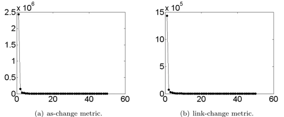
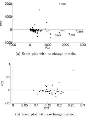
While the ISP-oriented approach presented in Chapter 2 gives a good in-sight on both major and minor events affecting specific portions of the Internet, approaching the root cause analysis problem from a “global perspective” usu-ally does not provide with such fine-grained results. On the other hand, the global approach is critical to identify major interdomain events, without any a-priori knowledge of the prefixes and/or the ASes involved. This thesis explores this perspective too. Specifically, Chapter 3 proposes a novel methodology based on the Principal Component Analysis (PCA), a well-known statistical technique that is commonly used to reduce the number of dimensions of multi-dimensional datasets in order to highlight the most significant trends of the data. Since the interdomain routing dataset is inherently multi-dimensional (in time, space, prefixes, observation points, ...), Chapter 3 suggests to apply the PCA to this dataset in order to identify the most significant contributors to the Internet dynamics.

BGP data collected by RIS’ and RV’s monitors provide a detailed view of the actual status of the interdomain routing. However, it does not report all the inter-AS peering relationships which are not active. For example, in “normal” conditions, backup links do not appear in the routing tables. Still, in order to understand the reasons behind some network events and to pre-dict the evolution of the routing when an event occurs, such information is actually very important. To cope with the intrinsic limitations of the RIS and RV dataset, Chapter 4 analyzes the data stored in the Internet Routing Reg-istry and describes how to extract peering relationships from routing policies collected within. Moreover, the proposed approach specifies how to solve in-consistencies among the distinct databases the IRR consists of. The obtained

(12)

results show that - even though the IRR data is often out-of-date, it still pro-vides a quite unique amount of topological information which usually does not appear in the global routing.

The research work described in the previous chapters relies on the assump-tion that Internet is a graph where ASes are atomic entities in the interdomain routing. However, recent papers [MFM+_{06, MUF}+_{07] show that such a model}

can mislead the understanding of the global routing behavior. Thus, Chapter 5 investigates this problem by measuring the route diversity that can be observed by passive remote vantage points, defining a methodology to compute it from a dynamic BGP dataset and characterizing it in terms of location of ASes in the Internet customer-provider hierarchy and choice of monitors.

The thesis ends with Chapters 6,7, which document forensic analysis of two well-know events that occurred at the beginning of 2007, where models, methodologies and tools described in the previous chapters are exemplified using real case studies.

(13)

Chapter 1

Background

1.1 Internet and Interdomain Routing

The Internet is divided into administrative domains called Autonomous

Sys-tems (AS), each adopting consistent routing policies. An AS is identified by a

number called Autonomous System Number (ASN ). Every AS contains one or multiple destination networks. Each destination network is represented by an IP address prefix. As of December 2008, there are about 30,000 Autonomous Systems and more than 250,000 prefixes.

The Border Gateway Protocol (BGP) [RL95, RLH06] is the routing proto-col used to exchange reachability information between ASes. Two ASes that exchange routing information using BGP are said to have a peering between them. The ASes having a peering with an AS A are termed peers (or

neigh-bors) of A. A BGP router stores in its Routing Information Base (RIB) the prefixes it can reach, and for each of them an AS-path. An AS-path is the

sequence of ASes used to reach the destination prefix. Routes are propagated by BGP messages called updates. BGP is an incremental protocol: once two BGP routers establish a peering, they exchange their whole RIB each other; this process is called table transfer. Further updates are sent only if a route changes, in response to network events (e.g., link failure, router reset, or policy change). Once a BGP router receives from any of its peers an update for a prefix p, it recomputes its best path towards p, possibly changes its own RIB and propagates the update to its peers.

Routing policies can be configured to decide which neighbors to send routes

(14)

customer-provider relationships. Such relationships define a hierarchy of all the ASes.

1.2 Interdomain Routing Data Sources

1.2.1 Actual Routing Data

To obtain information about the evolution of the Internet routing state, projects such as the RIPE NCC’s Routing Information Service (RIS) [roub] and the Uni-versity of Oregon’s RouteViews Project (RV ) [roua], spread around the world several passive collection boxes, called (Remote) Route Collectors (RRCs). Each route collector peers with several BGP routers, called Collector Peers (CPs) or monitors, belonging to various ASes. The routing tables of all RRCs and the updates they receive are periodically dumped, permanently stored, and made publicly available. Some collector peers provide information about all the prefixes on the Internet, while others only provide information about a subset of them. We call the former full collector peers, the latter partial

collector peers.

1.2.2 Internet Routing Registry

The Internet Routing Registry (IRR) [ripc, irra] is a large distributed reposi-tory of information, containing the inter-domain routing policies of many of the networks that compose the Internet. The IRR was established in 1995 with the main purpose to promote stability, consistency, and security of the global Inter-net routing. The IRR can be used by operators to look up peering agreements, to study optimal policies, and to (possibly automatically) configure routers.

The IRR consists of several databases, called (routing) registries. Some routing registries are maintained by Regional Internet Registry (e.g., RIPE [regc], ARIN [rega]) and contain information over wide geographic regions, while oth-ers are maintained by Local Internet Registries (e.g., VERIO [regd], LEVEL3 [regb]) and describe routing policies of the customers of a specific Internet Service Provider.

The registration and maintenance of routing policies are performed on a voluntary basis by network operators, who may register such policies at one or more registries. As a consequence, information in the IRR may be incorrect, incomplete, or outdated. Indeed, some large ISPs and Internet Exchange Points rely on the IRR for route filtering and their customers are required to document their policies in a registry.

(15)

The Routing Policy Specification Language

The routing policies stored in the IRR are described using the Routing Policy

Specification Language (RPSL) [AVG+_{99, MSO}+_{99] or its more recent}

vari-ant RPSLng [BDPR05], which introduces support to both multicast and IPv6. RPSL is an object-oriented language that defines 13 classes of objects. Rout-ing policies are described in the import, export, and default attributes of aut-num objects. In turn, aut-nums may reference other objects that con-tribute to the specification of the policies, such as as-sets and peering-sets. What follows is a portion of an RPSL aut-num object from the RIPE reg-istry which describes the inter-domain policies of AS137 (last updated 06/11/07). The portion of the import (export) attribute following the from (to) keyword is a very simple example of peering specification. The object indicates that AS137 accepts any route sent to it by AS20965 and by AS1299 and propagates to AS1299 all the routes originated by ASes belonging to the as-set named AS-GARR (an as-set is an RPSL object that specifies a set of ASes). This implies that AS137 has a peering with AS20965 and AS1299.

aut-num: AS137

import: from AS20965 action pref=100; from AS1299 action pref=100; accept ANY

[...]

export: to AS1299 announce AS-GARR [...]

changed: vincenzo.puglia@garr.it 20070611 source: RIPE

Peval and IRRd

Peval is a policy evaluation tool conceived to write router configuration

gener-ators and it is part of the Internet Routing Registry Toolset (IRRToolSet) [irrc] suite. Peval takes as input an RPSL expression and evaluates it by applying RPSL set operators (AND, OR, NOT) and by expanding as-sets, route-sets, and AS numbers into the corresponding sets of prefixes. Alternatively, Peval can stop the expansion at the level of ASes. The IRR data can also be accessed through the Internet Routing Registry Daemon (IRRd) [irrb], a freely available stand-alone IRR database server supporting both RPSL and RPSLng.

(16)

1.3 Principal Component Analysis

Principal Components Analysis (PCA) is a well-known statistical technique

used for understanding the variance of a given data set. PCA maps a set of points from a n-dimensional space into a new orthogonal n-dimensional space, where the variance of the original data along each axis is maximized. The axes of the new space are called principal components. The coefficients of the new reference axes are called loadings, and the projections of the original data onto these axes are called scores.

Given a m×n matrix X, where each row represents a point, PCA computes

n principal components vini=1 defined as follows: vk = argmax||v||=1||(XT −

!k−1

i=1 X

T_v

ivTj)v||. The principal components are the n eigenvectors of the

estimated covariance matrix and are ranked according to the amount of vari-ance they capture in the original data. The varivari-ance of each component is described by the corresponding eigenvalue. When the input matrix is zero-mean, the first principal component contains the most variance in the original data, and any other kth_{principal component - with k = 2, ...n - identifies the}

maximum variance in the remaining data, i.e. the original data after removing the contributions of the previous k − 1 components.

Typically, the first few principal components capture almost all the variance in the input dataset. Thus, PCA is usually applied for dimensionality-reduction of datasets to obtain more compact representations in lower dimensional sub-spaces, by keeping lower-order components and ignoring higher-order ones.

(17)

Part I

(18)

(19)

Chapter 2

Detecting and Analyzing

Inter-domain Events

Interdomain routes change over time, and it is impressive to observe up to which extent. Routes, even the most stable, can change many times in the same day and sometimes in the same hour or minute. Such variations can be caused by several types of events, e.g., the change of the routing policies of an ISP, the reboot of a router, or the fault of a link. Some events are physiological to the network, while others are anomalous.

In this chapter we do a step towards the identification of the cause of route changes, a problem that is attracting increasing attention from both researchers and network administrators. Namely, we propose a methodology for analyzing a given BGP route change in order to, at least partially, locate the event that triggered the change. The methodology is supported by an on-line service.

The main results presented in this chapter are also described in [CCD+_08,

CRC+_08].

This chapter is organized as follows. Section 2.1 describes previous work and our contributions to this research area. Sections 2.2 and 2.4 describe, re-spectively, the flow-based model and the methodology we defined. Our dataset is described in Section 2.3. Section 2.5 describes the BGPath´s user interface through a real usage scenario and provides a high level description of how the BGP data is processed. The underline algorithms are detailed in Section 2.6. The effectiveness of the methodology and the tool is discussed in Section 2.7 by means of simulation experiments and real world data analysis. Section 2.8 concludes this chapter.

(20)

2.1 Introduction

We consider the following scenario. A network administrator of an Internet Service Provider observes that one of the prefixes announced by its Autonomous System to the Internet had a BGP path change at a certain time. For example, prefix p announced by AS1 usually reaches AS4 passing through AS2 and AS3, while suddenly it started using a different path through AS5 and AS6. The network administrator would like to know why that change happened.

Previous Work

Recent works (e.g., [WMW+_{06]) underline the impact of routing changes in}

end-to-end performance. Also, this issue becomes much more important as services requiring almost constant delay, limited jitter and packet loss, gain popularity. Hence, many ISPs are interested in understanding what happens to their prefixes in the interdomain routing.

Actually, many research works studied BGP routing dynamics in the last few years. Their contributions can be broadly classified as follows. There are black-box approaches, that apply statistical techniques to group BGP updates into sets that are supposed to be triggered by the same underlying event. Ref. [XCZ05] uses the Principal Components Analysis, [ZYZ+_{04] uses}

statistics-based anomaly detection, and [ZRF05] exploits the wavelet transform. Other authors propose white-box approaches. In [FMM+_{04,CGH03,CSK03] streams}

of BGP updates are analyzed, correlating information across time, topology, collectors, and prefixes. Ref. [LNMZ04] describes an algorithm, that pinpoints the origin of routing changes due to a link failure or a link restoration, assuming shortest path routing. Finally, some authors (see, e.g., [WMRW05]) propose to add an infrastructure to the Internet in order to monitor route changes.

Those contributions generally aim at reporting a full set of events that hap-pened in the network in a given time slice. Roughly, updates are first grouped into clusters, and then events are detected by analyzing multiple clusters. In this modus operandi, the correlation between an update and an event can be biased by the a priori generation of the clusters.

Our Contributions

Taking into account the scenario described at the beginning of this section, we propose to tackle the problem from a different perspective. We assume the perspective of an ISP, that is not interested in what happens to the network in

(21)

general but is rather interested in what happens at a certain time to (some of) its own prefixes. Hence, instead of analyzing a bulk of updates for detecting events in the network, we analyze a specific BGP-update trying to locate its originating event.

In this chapter we present the following contributions. In Section 2.2, we show that BGP updates have a flow-based behavior, where the term “flow” is used with its graph-theoretic meaning. The collectors of updates are sources of flow and the ASes originating prefixes are sinks. Exploiting this property, we propose a flow-based model of BGP updates. As far as we know, this is the first time that BGP updates are modeled in terms of a flow system. As a side effect, we put in a flow-based perspective the concept of link-rank, defined in [LMZ04]. Further, this section introduces the new concept of global-rank. In Section 2.4, we propose a methodology for analyzing a given BGP route change c in order to, at least partially, identify and locate the event that triggered c. The cornerstones of the methodology are: (i) A data quality analysis for discarding unreliable data, extending the approach of [ZKL+_05].

(ii) A macro-events detection analysis, focused on local and global ranks. (iii) A fine-grained analysis that analyzes flow changes in a relevant part of the network. The methodology is illustrated by several examples from a reference week. The effectiveness of the methodology is discussed in Section 2.7 by means of simulation experiments and real world data analysis. Our data sources are described in Section 2.3.

The methodology described in Section 2.4 requires the analysis of huge amount of data, and hence it would be unfeasible if not supported by some automatic facility. We developed an on-line service that offers many tools to support the methodology. A prototype version is available at

http://nerodavola.dia.uniroma3.it/rca/

2.2 Flow-based Model of Inter-domain Routing

Dynamics

Several models have been proposed to study the evolution of interdomain rout-ing. Most of them assume that each AS can be collapsed into a single router, while others [MFM+_{06] represent the internal structure of each AS with}

differ-ent levels of accuracy. The first approach can be too coarse-grained to capture the impact of the internal routing of an AS on the evolution of the Internet. On the other hand, the second approach contrasts with the fact that the cur-rently available methodologies and data are not able to provide a fine-grained

(22)

complete and accurate description of the internal structure of an AS.

In this section, we introduce a model based on the concept of flow. The model is shown to be valid not depending on the internal structures of any AS. The validity of the model has the benefit of allowing correct deductions in Root Cause Analysis of interdomain routing. Of course, it also has the drawback of not capturing dynamics internal to an AS.

Basic Terminology

We consider the following sets. ASes is the set of all the known ASes, ASes =

{1, . . . , 65535}. Since we will consider a graph whose nodes are the elements

of ASes, the ASes will also be called vertices. T is the set of all the considered instants of time when a BGP update is received by a RRC from a collector peer. CP is the set of all the collector peer identifiers.

An AS-path (or simply path) π = (asn, . . . , as0) is a sequence of ASes,

where asi∈ ASes. as0 is called origin. The empty path is denoted by φ. AP is

the set of all known AS-paths. An edge is a pair (asi+1, asi) of ASes that are

adjacent in some AS-path. We consider edges as directed, i.e. (v, w) $= (w, v). We say that a path contains an edge, π ⊇ (asi+1, asi). Each collector peer cp

stores in its RIB the AS-paths it selects to reach all the observed prefixes. An update u is a quadruple (cp, p, π, t) where u.cp ∈ CP is the CP that collected the update, u.p ∈ P is the prefix contained in the update, u.π ∈ AP is the AS-path announced by the update, and u.t ∈ T is the time when the update has been collected. If u.π $= φ then u is an announcement, otherwise it is a

withdrawal. U is the set of all known updates. The last update u that collector

peer cp received for prefix p before time t is denoted #cp(p, t). Formally, #cp(p, t)

is such that #cp(p, t).t < t and !u ∈ U | u.cp = cp ∧ u.p = p ∧ #cp(p, t).t <

u.t < t.

A route change (or simply change) occurs every time a collector peer cp updates its route to a prefix p. Formally, a change c triggered by an update u is a quintuple (cp, p, πold, πnew, t), where πold is the path to prefix c.p that c.cp

uses before c.t (πold= #cp(p, t).π) and πnew is the path that c.cp uses after c.t

(πnew= u.π). If both c.πold$= φ and c.πold$= c.πnew, the route change is also

called path change.

Global, Local and Origin Ranks

We now define three concepts that will be crucial for the methodology described in Section 2.4, called local rank, global rank, and origin rank. While the first

(23)

has been introduced in [LMZ04], the others are, as far as we know, unexplored concepts.

Given a collector peer cp, the local rank of an edge e at time t - denoted by lrank(cp, e, t) - is defined as the number of prefixes whose path at time

t, as observed by cp, contains e. Observe that, since cp’s RIB can change

over time, the local rank depends on time (as well as on cp and e). Formally,

lrank(cp, e, t) = _|Pcp(e, t)|, where Pcp(e, t) = {p ∈ P | e ⊆ #cp(p, t).π ∨ ∃u =

(cp, p, π, t) ∈ U | u.cp = cp, u.t = t, e ⊆ u.π}.

Given a set of collector peers CP, the global rank of edge e at time t - denoted by grank(e, t) - is defined as the number of distinct prefixes p for which there exists at least one cp ∈ CP such that its AS-path towards p at time t contains

e. Also the global rank of an edge changes over time. Formally, grank(e, t) =_{|P (e, t)|, P (e, t) =} "

cp∈CP

Pcp(e, t).

Intuitively, while the local rank measures the number of prefixes that are observed passing through an edge by a single CP, the global rank measures the number of distinct prefixes that are observed passing through an edge by any CP ∈ CP. We stress that, since the global rank takes into account all the collector peers at the same time, it provides a way to analyze interdomain routing from a cross-vantage point perspective.

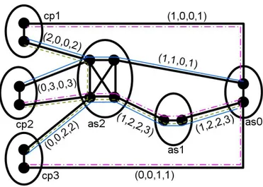
Fig. 2.1 illustrates the values of local and global ranks of the edges of a fragment of Internet at a certain time t. For example, the label (1, 2, 2, 3) on edge (as1, as2) states that lrank(cp1, (as1, as2), t) = 1 since cp1 sees just the

green dashed prefix traversing (as1, as2). Also, grank((as1, as2), t) = 3 since (as1, as2) is traversed by all three prefixes. Note that grank((as1, as2), t) $=_#

i=1,2,3

lrank(cpi, (as1, as2), t). Observe that, even if cp2and as2have multiple

peerings, according to our definitions, we labelled their pair only once. Since the local rank relies on a single vantage point cp, this metric can be biased by malfunctions of cp, while the global rank is more resilient to faults affecting only a small subset of all collector peers. Moreover, network-related issues (such as congestion or large scale attacks), which can impact the monitoring system as shown in [WZP+_{02], are less likely to affect the global}

rank metric, given the wide geographical distribution of the collector peers. Summarizing, the global rank allows us to cope with what can be broadly classified as “noise” within the collection system. On the other hand, the local rank provides fine-grained information which is valuable to analyze a network event which only involves a relatively small portion of the Internet. In this

(24)

Figure 2.1: Big points represent routers, thick solid black lines represent IBGP or EBGP peerings between routers, and ellipses represent ASes. ASes cpi, i∈ {1, 2, 3}, contain

col-lector peers. Each edge e inter-AS is labelled with a quadruple containing lrank(cp1, e, t),

lrank(cp2, e, t), lrank(cp3, e, t), and grank(e, t). AS as0originates three prefixes. Thin blue solid, green dashed, and pink mixed lines represent the routes to such prefixes observed by collector peers.

case, in fact, the evolution of grank could be misled by collector peers which do not observe the event. Overall, local and global ranks provide complementary benefits and partially compensate each other’s weaknesses.

Finally, given a collector peer cp we define the origin rank of AS v at time t as θ(cp, v, t) = |P (cp, v, t)|, where P (cp, v, t) = {p ∈ P | #cp(p, t).π =

(asn, ..., v), n≥ 0 ∨ ∃u ∈ U | u.cp = cp, u.t = t, u.π = (asn, ..., v)}. Notice

that function θ(cp, v, t) represents the number of prefixes that, at time t, are known by cp as originated by AS v. As an example, consider collector peer cp1

in Fig. 2.1. θ(cp1, as0, t) = 3 and θ(cp1, as, t) = 0∀as $= as0.

We denote by lrank (grank) the weighted average of the local (global) rank of an edge over time.

Flows of Prefixes

Whenever a negative (positive) variation of a local rank is observed during a given time interval, it is interesting to further investigate where prefixes “went

(25)

to” (“came from”). Intuitively, prefixes move around on the AS graph, as well as water would move in a pipe network. This analogy introduces the concept of flows of prefixes. Tracking the flow of prefixes along different paths can be done by adapting the well-known concept of flow system to the interdomain routing.

Given a directed graph G = (V, E), a specific vertex asncalled source, and

a mapping between vertices and flow absorption g : V → Z, then a flow system is a function f : E → Z where ∀v ∈ V, v $= asn, # (u,v)∈E f (u, v)₋ # (v,w)∈E f (v, w) = g(v).

Theorem 1 shows that functions lrank(cp, e, t) and θ(cp, v, t) define a flow system at time t. Intuitively, we have that the source of the flow is the AS

asn in which cp is located, and the sinks are all the ASes that originate some

prefixes, as observed by cp. A prefix contributing to one unit of the local rank of some edge e contributes also to one unit of the amount of flow traversing e. As an example, consider collector peer cp1(in asn) of Fig. 2.1. For instance, for

as2, we have that the sum of the local ranks over incoming edges (cp1, as2) is

2, and the sum of the local ranks over outgoing edges (as2, as0) and (as2, as1)

is 2. On the other hand, since as2does not originate any prefix known to cp1,

θ(cp1, as2, t) = 0. Hence, the flow around as2is conserved.

Theorem 1. At a specific time instant, functions lrank and θ define a flow

system.

Proof. Select a specific instant t and a specific collector peer cp. Consider the

value x = θ(cp, v, t) of function θ for any vertex v. Because of the definition of

θ we have that for each unit of flow in x there exists a prefix p such that either p_{∈ P | #}cp(p, t).π = (asn, ..., v), n≥ 0 or ∃u ∈ U | u.cp = cp, u.t = t, u.π =

(asn, ..., v). In both cases we identify an update u that is received from asnand

originates from v. Consider a sequence of two consecutive edges (asi+1, asi)

and (asi, asi−1) contained in u.π, u contributes with one unit of flow both to

lrank(cp, (asi+1, asi), t) and to

lrank(cp, (asi, asi−1), t). Hence, for each AS asi $= v, u does not affect the

balance of asi. This means that for each vertex v, if we consider only paths

not ending with v we have #

w∈V

lrank(cp, (w, v), t) = #

w∈V

(26)

Now, each path ending with v increases both the flow on an incoming edge,

lrank(cp, (w, v), t), and θ(cp, v, t). Then we conclude that,_{∀v ∈ V ,}

#

w∈V

lrank(cp, (w, v), t) = #

w∈V

lrank(cp, (v, w), t) + θ(cp, v, t).

Observe that Theorem 1 holds even if some ASes perform BGP prefix ag-gregation. In fact, in this case a collector peer is unable to track all the prefixes contained in the aggregation and the aggregated prefix counts for just one unit of flow.

We stress that functions grank and θ do not define a flow system. As a counterexample, consider again AS as2in Fig. 2.1. We have that the algebraic

sum of the global ranks of the edges incident on as2is not zero.

Theorem 1 is useful to depict a snapshot of the network at a given instant, while in Theorem 2 we relate the flows of two different instants of time. We define the functions

∆lrankt+τ

t (cp, e) = lrank(cp, e, t + τ) − lrank(cp, e, t)

that captures local rank variations (flow variations) between t and t + τ, and the function

∆θt+τ

t (cp, v) = θ(cp, v, t + τ) − θ(cp, v, t).

that accounts for the variation in the number of prefixes that are known by cp as originated by v.

Theorem 2. Functions ∆lrankt+τ

t (cp, (v, w)) and

∆θt+τ

t (cp, v) define a flow system.

Proof. For the sake of simplicity, we use l((v, w), t) in substitution of lrank(cp, (v, w), t). _{∀v ∈ V :} # w∈V ∆lrankt+τ t (cp, (w, v)) − # w∈V ∆lrankt+τ t (cp, (v, w)) = # w∈V l((w, v), t + τ )−# w∈V l((v, w), t + τ )+ − # w∈V l((w, v), t) + # w∈V l((v, w), t) = θ(cp, v, t + τ )− θ(cp, v, t) = ∆θt+τ t (cp, v).

(27)

Observe that, because of the high connectivity of the Internet, a collector peer is likely to be able to reach a constant number of prefixes over time. Also, each of such prefixes is typically announced always by the same origin. Hence, we expect that function ∆θt+τ

t (cp, v) is zero in most cases. That is, we expect

that the flow is overall conserved over time.

2.3 Our Dataset

Our work (and BGPath) relies on BGP data obtained from both RIS [roub] and RV [roua]. Overall, these projects (as of February 2007) provide 526 col-lector peers, 30% of which are full colcol-lector peers.

Examples and statistics presented in this chapter refer to the data collected from 12/26/2006 to 01/02/2007. We chose this time interval, referred to as

reference week, because it featured massive BGP activity due to Taiwan

earth-quakes and it preceded the fix of a bug affecting RIS collectors. The reference week contains 320, 678, 893 updates (∼ 46M updates/day on average) with 7, 537, 378 distinct paths on 70, 078 distinct peerings and 24, 493 distinct ASes. The number of observed prefixes is 235, 725.

2.3.1 Reliability Screening

In order to discard data coming from faulty or misconfigured collector peers, we periodically perform a data cleaning step, called Reliability Screening. The unreliability of a collector peer can be due to several reasons, including bugs in routing or collection software (see [Kon03] for details), major asynchronies be-tween the collector peer and its route collector, and poor standard compliance (e.g., some vendors do not implement highly recommended optional timers).

The screening of a collector peer cp over a time interval [tstart, tend] is

executed as follows: (i) we make a local copy of the RIB of cp at tstart, (ii) we

modify the copy according to the updates collected by cp during [tstart, tend],

(iii) we compare the modified copy to the RIB dumped by cp at tend, (iv) we

decide if cp is reliable evaluating the ratio between number of mismatches and its average RIB size.

Reliability Screenings performed during several experiments led to the de-tection of a major problem that affected RIS route collectors since May 2005. Overall, the problem affected 44 collector peers, 12 of which were full collec-tor peers. Contacting the RIS maintainers resulted in fixing this problem by January 2nd_{, 2007.}

(28)

2.4 Methodology to Detect and Analyze Inter-domain

Events

We present a methodology for analyzing a given route change c within the model of Section 2.2. The goal is to identify the portion of the Internet where the event that caused c happened. The methodology consists of three steps.

Collector Peer Check and Selection: We check the availability of collector peers,

and we select a set of collector peers that will be considered in the following analysis. Macro-Events Detection: We look for patterns of macro-events, by exploiting the global and local ranks of some edges. This step relies on Theo-rems 1 and 2. Fine-Grained Analysis: If no macro-event has been detected in the previous step, we perform a fine-grained analysis based on several patterns that are consequences of Theorem 2.

Before starting the description of the steps, we underline an issue related to the timing of network events. In several points of the methodology, we analyze what happens in a time interval including the time c.t of the input route change. According to [LWVA01], we consider the time interval [c.t − ∆, c.t + ∆], with ∆ =180 seconds, as a reasonable compromise between accuracy and feasibility and we refer to it as Tc.t. However, the methodology does not depend on this

choice.

2.4.1 Collector Peer Check and Selection

Before starting the analysis of the route change c, the methodology requires to execute the Reliability Screening (Section 2.3.1) in order to discard all the unreliable CPs.

Also, collector peers may reboot. If the collector peer c.cp that receives

c has a reboot in Tc.t, we interrupt the analysis because the data collected

through c.cp may be too noisy. Moreover, in the analysis of c, we will rely not only on c.cp, but also on other collector peers. Hence, in this step we look for all the collector peers that had a reboot in Tc.t. Information extracted from

those collector peers is not further considered. We detect a reboot by either analyzing BGP session state messages, when available, or by seeking for table transfers using the algorithm described in Section 2.6.1.

Among all reliable collector peers without any reboot in Tc.t, we select

those that belong to the ASes of the paths c.πoldand c.πnew, because they are

the most relevant for the subsequent analysis since they provide the closest perspective to analyze c.

(29)

2.4.2 Macro-Events Detection

In this step we try to relate c to a macro-event by performing first a global rank analysis and then a local rank analysis. We regard as macro-events those which affect either the physical or the logical network topology (e.g. an interdo-main link fault/restoration, a BGP router fault/restoration, or a BGP session shutdown/setup).

The evolution of the global rank grank(e, t#_{) with t}#_{∈ T}

c.t is considered for

each edge e in c.πold and c.πnew. Namely, we check if some edge e in c.πold

or in c.πnew has a relevant global rank variation and has a value near to zero

in Tc.t. This occurs when no collector peers see any prefix passing through

e, and it is a reasonable evidence that e is involved in some way in the event

that caused c. We identified three patterns of global rank evolution: (p1) a sudden loss of all prefixes, (p2) a sudden gain of new prefixes starting from 0 prefixes, or (p3) a sudden loss (gain) followed by the resume of the previous situation. Each patter possibly refers to different types of macro-events. E.g. (p1) describes an interdomain link e that fails and loses connectivity to all the prefixes. Once fixed, prefixes might be routed through e again (p2). According to our experience, both gains and losses usually occur within short time periods, due to BGP convergence time (see [LWVA01]). We relate macro-events to the evolution of the global rank of an edge e because it provides a global perspective given by the simultaneous views of e from several collector peers. As the number of collector peers that can see e decreases, this global perspective is more biased. In order to cope with this behavior, we define the rank diversity. The rank diversity of e is a pair .n, σx/x/, where n is the number of collector

peers cp having lrank(cp, e) > 0, σx and x are the standard deviation and the

average, respectively, of such lrank(cp, e). We say that the rank diversity is

high if n is large and σx/x is small. In fact, if n is large we have many collector

peers that can see e, and when σx/x is small we have that the collector peers

see a similar number of prefixes through e. The global rank analysis provides more valuable information on edges having higher rank diversity.

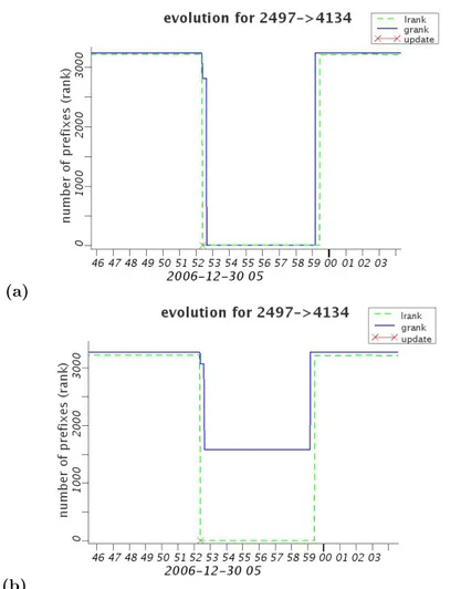
As an example, we analyze the path change c affecting the prefix c.p = 202.41.242.0/24, with c.πold= (2497, 4134, 4847, 37942) and c.πnew= (2497,

2914, 4134, 4847, 37942), observed by c.cp = 198.32.176.24 at time c.t = UTC 30/12/06 05:52:24. First, we check collector peers availability. We identify

∼ 20 collector peer resets in Tc.t and discard data coming from these CPs.

Then, we evaluate the global rank of the edges in c.πold and c.πnew. We have

that grank(e) = 0 in Tc.t, with e = (2497, 4134). Since grank(e) = 3, 166,

(30)

(a)

(b)

Figure 2.2: Functions grank (solid black) and lrank (dashed gray) of (2497, 4134). (a) With Reliability Screening. (b) Without Reliability Screening.

.7, 8.2%/. Hence, there are many (namely, 7) collector peers that can see e,

with a similar number of prefixes. So we consider its global rank trustworthy. This analysis suggests with reasonable confidence that the path change c has been triggered by a macro-event on edge e.

(31)

This example also shows the importance of the Reliability Screening. In fact, performing the same analysis skipping such a step, we obtain the evolution of grank(e) shown in Fig. 2.2.b. In this case, because of the noise generated by the unreliable RRCs, grank(e) never decreases below 1, 580, making the macro-event less visible.

Theorem 1 suggests that whenever there are multiple edges with grank = 0 in either c.πoldor c.πnew the most likely responsible for the macro event is the

edge closest to c.cp.

If the global rank analysis ends up with no candidates, we analyze each selected collector peer separately, by looking at the evolution of the local rank in Tc.t. On edges in c.πoldand c.πnew, we search for the same patterns as above.

Generally, we trust grank(as1, as2) more than lrank(cp, (as1, as2)), unless

cp belongs to as1 and provides its full routing table. In fact, we consider a

collector peer an authoritative source of information on the AS it belongs to. Otherwise, any inference supported only by local rank analysis requires further investigation.

Section 2.6.2 describes how we compute global and local ranks.

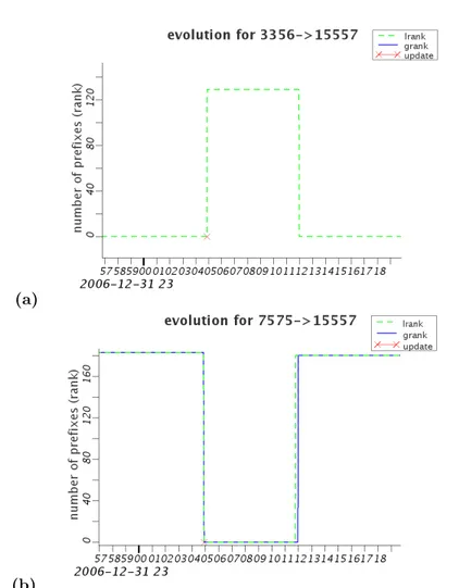
As an example, we analyze the path change c, where c.p = 80.124.192.0/19,

πold = (7575, 15557, 8228), πnew = (7575, 2914, 3356, 15557, 8228), c.cp =

198.32.176.177, and c.t = UTC 01/01/07 00:04:53. According to the Collector Peer Check, all the collector peers are available in Tc.t. We evaluate the global

rank of all edges belonging to c.πoldand c.πnew, and we have that grank(e) = 0

in Tc.t, where e = (7575, 15557). Note that grank(e) = 148. Unlike the

previous example, the rank diversity of e is low (.2, 0.1%/), as the edge is seen by only two collector peers, both belonging to 7575. So its global rank is not worthy. As a consequence, we analyze lrank for c.cp. Being c.cp in the left node of e, it is in the best position to observe routing events affecting e. Fig. 2.3 illustrates the evolution of lrank(c.cp, e), and grank(e) for e = (7575, 15557) and e# _{= (3356, 15557). It is interesting to notice that a relevant number of}

prefixes moves from an edge to the other (Theorem 2). From the information extracted, we can deduce with reasonable confidence that the path change c has been triggered by some macro-event affecting edge e.

2.4.3 Fine-Grained Analysis

If the Macro-Event Analysis doesn’t identify any cause for the route change

c, we examine flow changes in order to capture routing events which don’t

affect the interdomain topology. Namely, we look for events (e.g., BGP policy changes) that in general do not impact all the prefixes passing through an

(32)

(a)

(b)

Figure 2.3: Functions grank (solid black) and lrank (dashed gray) of (3356, 15557) (a), and (7575, 15557) (b).

interdomain link, but only a subset of them.

In the Fine-Grained Analysis we investigate flow changes on the whole Internet. However, in our experience, a flow change can spread over a very large portion of the Internet, making the analysis unfeasible. Thus, we focus on a fraction of a flow change, introducing the concepts of path compatibility

(33)

and restricted flow.

Two paths π1 and π2 are compatible (π1'( π2) when they share a common

left subsequence of at least two ASes (i.e. they share the first edge). A restricted

flow ∆t+τ

t fˆP(cp, (u, w)) is a flow defined on a subset P ⊆ P of the prefixes. We

consider especially interesting the restricted flow on prefixes that experienced, in Tc.t = [t, t + τ], a change whose either the old or the new path is compatible

with a given path π. In fact, such a restricted flow can be used to study routes coming from (moving to) π. Formally, we evaluate ∆t+τ

t fˆP(cp, (u, w)), with

P ={p | #cp(p, t).π $= #cp(p, t + τ).π ∧ (#cp(p, t + τ).π '( π ∨ #cp(p, t).π '( π)}.

For example, we analyze the path change c, where c.p = 202.59.174.0/24,

c.πold = (16215, 3549, 5511, 4761, 17727), c.πnew = (16215, 3549, 3320, 4761,

17727), c.cp = 80.81.192.143, and c.t = UTC 12/27/06 10:06:17. After an unsuccessful Macro-Events Detection, we proceed with the present step.

We try to track the rearrangement of the prefixes routed away from c.πold

(onto c.πnew). Thus, we compute the previously defined flow ∆t+τt fˆP where π =

c.πold(c.πnew). In our example we have that prefix 202.57.0.0/24 has, in Tc.t, a

path change from (16215, 3549, 5511, 4761, 17658) to (16215, 3549, 7473, 4761, 17658). The old path is compatible with c.πold((16215, 3549, 5511, 4761, 17658)

'( c.πold). Hence, it is part of the set P (also containing 740 other prefixes) that

we use to compute the restricted flow. Observe that, in any restricted flow, edges with a positive flow value describe where prefixes leaving paths compat-ible with π are re-routed to. Thus, we focus on these edges to analyze prefixes that left c.πold (π = c.πold). On the other hand, negative flow values indicate

where prefixes moving on paths compatible with π come from. Therefore, we focus on these ones to study prefixes that move onto c.πnew(π = c.πnew).

We build a restricted flow graph consisting of edges having ∆t+τ

t fˆP > 0

(∆t+τ

t fˆP < 0). Fig. 2.4 outlines a sketch of the restricted flow graph computed

on c.πoldfrom our example. The graph visualizes how prefixes in P moved from

edges in c.πold (red-colored, within the box) to the other edges (green-colored,

outside the box). For the sake of clarity, Fig. 2.4 omits edges with negligible flow values. Notice that most prefixes move away from the first two edges of

c.πold. This is mainly a consequence of flow systems behavior: the flow is more

likely to be high on edges closer to the source (collector peer).

Observe that a lot of prefixes move from (3549, 5511) to edges (3549, 3320), (3549, 3491), and (3549, 7473). Also, those prefixes are still routed through AS 4761 (edges (3320, 4761), (7473, 4761), and (3491, 4761)). We argue that this happens due to some event on (3549, 5511, 4761), since multiple events on (3549, 3320, 4761), (3549, 3491, 4761), and (3549, 7473, 4761) are much less

(34)

3320 16215 3549 4761 17727 7473 3320 3491 5511 6775 13285 2914 174

Figure 2.4: Green edges and their end-vertices are a portion of the restricted flow graph. Path π = c.πold is also displayed (highlighted in the box) for convenience. Thicker lines

represent edges with higher value of ∆t+τ_t fˆP

likely to occur concurrently. However, we cannot further distinguish if c hap-pens because of a routing event on either (3549, 5511) or (5511, 4761). We generalize the above discussion by considering the nodes mo and mi in π

hav-ing, respectively, maximum outgoing flow and maximum incoming flow in the restricted flow graph. The output set of candidates is the subpath (mo, . . . , mi)

of π.

There are some border-line cases to consider. For example, in case two vertices have maximum outgoing (incoming) flow, we can break the tie con-sidering the largest possible candidate set. As another example, there can be many vertices that have similar values of outgoing (incoming) flow. In this case our approach allows to deepen the analysis picking one of the path changes that involve maximum flow vertices and applying the same methodology iteratively on that change. This shift of focus makes our methodology inherently iterative, and allows to cope with the “induced instabilities” problem (see [FMM+_04]),

overcoming a common limitation of inference systems, which are usually able to locate causes of a route change only on the new or the old path.

(35)

2.5 BGPath: Online Tool to Support the Analysis of

Network Events

In order to automatically compute the metrics our methodology relies on, we developed a BGPath, a publicly available system that combines data collected by multiple distributed monitors, checks the reliability of available data sources, and estimates the usage of interdomain links. BGPath also graphically dis-plays detailed and aggregated information about a user-specified route change. This section describes the architecture of the service and how it supports the analysis of a route change.

2.5.1 Analyze a Route Change Using BGPath

Through the following scenario, we show how BGPath effectively supports the analysis of a route change in order to (at least partially) identify its root cause. For a complete description of the approach, see Section 2.4.

Assume that a network operator is interested in monitoring the prefix

p = 159.14.0.0/16. In particular, he knows that, on t =Jan 1st _{2007, p}

under-went the route change c displayed in Figure 2.5, where the old path c.πold =

(15837, 8881, 2914, 10910, 7328) and the new path c.πnew=(15837, 8881, 3356,

12178, 7328). Note that some exiting tools (e.g., BGPlay [bgpb, bgpc]) can be used to graphically browse through and select specific route changes.

In order to provide a network operator with a familiar representation of the portion of the Internet topology involved in the change c, BGPath draws c.πold

and c.πnew according to the customer-provider hierarchy (see e.g., [Gao01]).

Namely, tier-1 ISPs are represented by the top nodes in the graph, and cus-tomers are placed just below according to their position in the hierarchy. In Fig-ure 2.5, for example, the two top ASes are tier-1 providers (NTT and Level3). Besides being natural for an operator, this representation is also helpful to understand the relevance of network events related to the route change. In fact, [ZZM+_{05] shows that events located in different levels of the hierarchy}

usually have significantly different impact on the network. Section 2.6.3 de-scribes the visualization algorithm.

According to our approach, we first check the reliability of the collector peers which observed the route change c at the time t (CPc,t). Namely, we

are interested in whether the CPs ∈ CPc,t were involved, at any time close

to t, in events (e.g., a reboot) that could affect the quality of the BGP data collected. The reliability information is displayed for convenience in the left panel of BGPath’s main window, so the user can easily check it at a glance.

(36)

Figure 2.5: A route change c displayed by BGPath. Edges in the old path are represented by dashed lines, while edges in the new path are drawn with solid lines. Data about c are reported in the top of the window. The left panel contains a list of collector peers which observed c and the ASes they belong to, grouped by the route collectors they peer with. These collector peers are also marked by eye-shaped icons.

The ability to spot potentially unreliable data sources gives the user a high level of trust on the analysis of the change c. Thus, we believe it is a key step of our approach and a very important feature of BGPath. As far as we know, no other tools provide such an information. Note that BGPath only identifies possibly unreliable data sources, but it does not filter out the data they provide. Section 2.3 explains how we check the reliability of a collector peer by evaluating the consistency of the data it provides, while Section 2.6.1 details how to identify BGP table transfers associated with BGP session resets. To assess the scope of the route change c, the network operator can visualize the history of all routes chosen by c.cp to reach p within a fixed time window around t. Figure 2.6(a) shows the transition from c.πold =(15837, 8881, 2914,

(37)

(a)

(b)

Figure 2.6: Two examples of the path evolution plotted by BGPath. Time on the x axis, a set of distinct paths on the y axis. The label “---” denotes the empty path. (a) A prefix experiencing a short-lived path change. (b) A prefix whose path changed many times within a short time interval.

10910, 7328) to c.πnew(15837, 8881, 3356, 12178, 7328) at time t. Note that c.cp

switches path to the prefix p only twice (from c.πoldto c.πnewand back) within a

short time interval. Instead, Figure 2.6(b) shows an unstable prefix which keeps flapping between path (6067, 3549, 137) and (6067, 174, 137). Hence, looking at the path evolution, it is possible to verify whether the analyzed route change is part of any specific pattern of changes, e.g. if it is just a temporary oscillation, or if it belongs to a persistent dynamics. The visualization of path evolutions is also extremely useful to detect sequences of routing changes due to BGP path exploration. This way the user can verify whether the route change c in input was induced by path exploration. Finally, the interface of the tool also allows the operator to select other prefixes announced by the same origin AS, and to plot their path evolution within the same chart. Thus an ISP can monitor the

(38)

behaviors of different prefixes it announces on the network, and the impact of per-prefix routing policies (e.g., interdomain traffic engineering configurations). Once assessed the reliability of data sources and the scope of the route change c, the network operator can analyze the evolution of the number of prefixes routed through every edge e affected by c (i.e. belonging to either

c.πold or c.πnew) in order to have a rough estimate of the traffic load born by

e. BGPath plots both grank and lrank evolutions for all visualized edges.

For example, Figure 2.7(a) shows that, according to both lrank and grank,

e = (10910, 7328) carries a steady quantity of prefixes over time, but exhibits a

discontinuity right at time c.t. For a couple of minutes, in fact, all the prefixes that passed through e moved somewhere else. Since more than 20 collector peers contribute to the global rank, this discontinuity is an evidence of some problem affecting e. Zooming in the lrank(e) plot, Figure 2.7(b) exhibits lack of synchronization between lrank and grank. Note that, in general, grank experiences a delay in recording a “negative” variation, while it is much more reactive in recording a “positive” variation, with respect to lrank. This is a consequence of the aggregated nature of grank: since it is defined to be a set-theoretical union, grank(e) does not drop to a lower value until all collec-tor peers stop using e to reach at least one prefix. Since worldwide spread collector peers are not perfectly synchronized, the grank is bounded to the slowest-reacting collector peer. Symmetric considerations apply to “positive” variations. Figure 2.7(c) exemplifies grank and lrank of a link probably expe-riencing some faults.

At this point, the network operator has an evidence of some event happened on e. This event caused, for a very short time interval, all the prefixes passing through e to change their routes. Prefix c.p is among them. The user can further deepen his analysis by exploring different time intervals, in order to check if the shortage occurred again.

2.5.2 A Stream-Based Approach to Process Inter-domain

Data

The approach described in Section 2.5.1 relies on the availability of informa-tion such as local and global ranks of all the interdomain links in Internet and reliability of all the available collector peers. This information is not explicit in BGP raw data (i.e., RIB dumps, updates, and session logs), and efficiently computing it is critical for a near real-time analysis of route changes. This sec-tion provides a high level descripsec-tion of how BGPath processes the input data within reasonably strict time constraints. Section 2.6 details the algorithms we

(39)

(a)

(b)

(c)

Figure 2.7: Local and Global ranks. (a) A link with a short service discontinuity. (b) Zoom of the discontinuity. (c) A link with some malfunction.

(40)

Figure 2.8: Information flow of the computation process.

devised and their performance evaluation.

The key idea to speed up the computation is treating input and output data as streams: this way, the current value of the metrics is incrementally updated and pushed into the output stream at a little cost, in terms of both time and memory requirements. As a drawback, this approach requires to scan the output stream in order to access a specific part (e.g., when searching for the grank of an edge at a specific time), potentially decreasing response time. We deal with this issue by partitioning and indexing the output stream.

Figure 2.8 outlines the building blocks of the computation process. Namely, the input data stream is handled as follows: (i) Retrieving: RIB dumps, up-dates, and session logs (if available) are collected from several data sources. (ii) Reliability Screening: collector peers are periodically checked for consis-tency. Those found inconsistent are temporarily disregarded (see Section 2.3). (iii) Computing Ranks: taking consistent BGP routing data (RIB dumps and updates) as input, the algorithms described in Section 2.6.2 compute local and global ranks for all the collector peers and for all the edges in the Internet. (iv) Finding Table Transfers: in parallel, table transfers and their alleged du-ration are identified by applying the algorithm in Section 2.6.1 to consistent BGP data. Then, identified table transfers are combined with session logs (if available).

Note that, since the available data sources currently provide BGP updates grouped into chunks, BGPath has to fully process a chunk before another one

(41)

comes out of the input stream, in order to satisfy the strictest time constraint. Given the average per-chunk performance reported in Section 2.6, BGPath is able to process a 15-minute chunk in less than 3 minutes, including the time to retrieve the input data.

Also, the space to store both raw and computed data is an important con-straint. A week of data costs approximately 65GB. Observe that data com-pression would sacrifice CPU time for space, delaying data processing and slowing down query responses. To limit storage requirements, BGPath cur-rently manages data within a fixed-length sliding window spanning back up to

n days. Currently, we keep one month of data (i.e., n = 30) available for user

queries.

We evaluated the performance of our tool using a Linux testbed with the following hardware: 2x Intel Xeon 2.80GHz CPUs, 512KB cache, and 4GB RAM. Note that this is an average platform, thus any common machine can effectively run BGPath.

2.6 Algorithms

This section describes the algorithms we devised to identify table transfers and compute local and global ranks, that fulfill the time constraints outlined in Section 2.5.2. Performance analyses illustrated in this section will show that both the algorithms have reasonable time and memory requirements to be executed on an average machine. We also describe how to visualize AS-path changes in order to support the analysis of network events.

2.6.1 Identification of Table Transfers

[WZP+_{02] shows that BGP sessions between route collectors and collector}

peers can undergo frequent resets. Observe that, after the fault of a session between a collector peer cp and its route collector rc, the data collected by rc are out of sync with cp, until the session is restored and cp sends its whole BGP table to rc. Hence, rank values can be misleading in the time interval between the fault and the end of the subsequent table transfer. Note that this issue especially affects local ranks, while global ranks are less sensitive to the contribute of a single collector peer.

When available, BGP state messages provide an evidence of session resets by recording transitions from/to the BGP state 6=Established [RLH06]. Un-fortunately, only RIS collector peers supply state messages. Thus, we devised Algorithm 1 in order to identify, with a reasonable accuracy, all the BGP table

(42)

transfers occurred between collector peers and route collectors in a given set of route changes. We stress that our algorithm is valuable even when state mes-sages are available, because it also estimates the duration of a table transfer. This information cannot be extracted from state messages and it is necessary for pinpointing updates caused by resets to disregard them during the analysis. Although [ZKL+_{05] has already described an approach to identify table}

transfers, we found out that it does not scale over a large set of collector peers. Namely, even if [ZKL+_{05] does not formalize the computational complexity}

analysis of the proposed algorithm, it is easy to find that it requires O(nωσ) time and Ω(ωσ) space, where n is the number of processed changes, σ is the maximum number of changes per second, and ω is the width of a time window that is used to scan the changes (whose maximum size is two hours). Although time complexity is feasible if ωσ is o(n), processing a huge set of data requires a lot of memory. Algorithm 1 was designed to tackle this space complexity problem.

Given a stream of route changes, Algorithm 1 pinpoints a table transfer from any collector peer, with an approximation of the start time of the transfer and its duration.

The main intuition is that, within a reasonably short time interval, a col-lector peer usually sends updates for a set of prefixes that is relatively small compared to its full BGP table. When most of the full RIB is announced within a short time, we guess the occurrence of a table transfer. Algorithm 1 slides a fixed-width time window over the BGP update stream and compares the number of distinct prefixes sent by a collector peer in the window to its full RIB size.

Since the RIB size varies over time, we define a function ρ(cp, t), ρ : (CP ×

T ) → R that accounts for the evolution of the RIB size of cp, and a threshold

ratio δ. Every time that the window contains more than δρ(cp, t) distinct prefixes, the algorithm alerts an alleged table transfer. We define ρ as the weighted average of the RIB size of cp until time t, where the weights are the amounts of time within which the RIB had a certain size. This choice has at least two advantages. First, it is computable in O(1) time, without memory penalties (only one value per collector peer needs to be retained in memory). Second, it is low-sensitive to short-lived hijacking, even when they involve many prefixes. Namely, let tibe the time of the i-th change of the RIB size of cp, let

Root cause analysis and forensics in interdomain routing: models, methodologies and tools

ROMA

TRE

Roma Tre University

Ph.D. in Computer Science and Engineering

Root Cause Analysis and Forensics

in Interdomain Routing:

Models, Methodologies and Tools

Tiziana Refice

Root Cause Analysis and Forensics

in Interdomain Routing:

Models, Methodologies and Tools

Contents

I

Models, Methodologies and Tools

5

II Case Studies

99

Appendices

137

Introduction

Chapter 1

Background

1.1

Internet and Interdomain Routing

1.2

Interdomain Routing Data Sources

1.2.1 Actual Routing Data

1.2.2 Internet Routing Registry

1.3

Principal Component Analysis

Part I

Chapter 2

Detecting and Analyzing

Inter-domain Events

2.1

Introduction

Previous Work

Our Contributions

2.2

Flow-based Model of Inter-domain Routing

Dynamics

Basic Terminology

Global, Local and Origin Ranks

Flows of Prefixes

2.3

Our Dataset

2.3.1 Reliability Screening

2.4

Methodology to Detect and Analyze Inter-domain

Events

2.4.1 Collector Peer Check and Selection

2.4.2 Macro-Events Detection

2.4.3 Fine-Grained Analysis

2.5

BGPath: Online Tool to Support the Analysis of

Network Events

2.5.1 Analyze a Route Change Using BGPath

2.5.2 A Stream-Based Approach to Process Inter-domain

Data

2.6

Algorithms

2.6.1 Identification of Table Transfers