Analysing technical analysis

(1)

Economics Department

Analysing Technical Analysis

S

pyros

S

kouras

ECO No. 97/36

EUI WORKING PAPERS

(2)

European University Institute 3 0001 0036 6990 2 © The Author(s). European University Institute. version produced by the EUI Library in 2020. Available Open Access on Cadmus, European University Institute Research Repository.

(3)

EUROPEAN UNIVERSITY INSTITUTE, FLORENCE

ECONOMICS DEPARTMENT

EUI Working Paper ECO No. 97/36

Analysing Technical Analysis

Spyros Skouras

UP 3 3 0 EUR

BADIA FIESOLANA, SAN DOMENICO (FI)

(4)

No part of this paper may be reproduced in any form without permission of the author.

© Spyros Skouras Printed in Italy in December 1997

European University Institute Badia Fiesolana I - 50016 San Domenico (FI)

Italy © The Author(s). European University Institute. version produced by the EUI Library in 2020. Available Open Access on Cadmus, European University Institute Research Repository.

(5)

Analysing Technical Analysis

Spyros Skouras*

email: skouras@datacomm.iue.it

This version, November 1997

A b stra ct

This paper proposes an expected utility framework for the treatment of theoretical and empirical issues in technical analysis. Circumstances are found in which a technical analysts’ behaviour is ’rationalisable’ and schemes for learning such rational behav iour are considered. The decision theoretic perspective developed is shown to be useful in formalising a measure of trading rule optimality, in creating improved rules and in using these rules to create powerful model specification tests. The framework is shown to be useful in relating the efficacy of technical analysis to the efficiency of financial markets and an empirical analysis of this relationship is provided.

'T his paper was previously circulated with the title ’An (Abridged) Theory of Technical Analysis’. The research leading to this paper was supported by a grant from I.K.Y.. Thanks are due to Dave Cass, Alex Gumbel, Mark Salmon and particularly Ramon Marimon for useful comments and suggestions on previous versions of this paper. © The Author(s). European University Institute. version produced by the EUI Library in 2020. Available Open Access on Cadmus, European University Institute Research Repository.

(6)

1 In trod u ctio n and M otivation

Economists, until recently, have viewed technical analysis (or chartism) with a great degree of skepticism. Indeed, typically technical analysis was treated as an irrational mode of behaviour th at can be approximated suf ficiently well by the conceptual construct of a ’noise trader’ (Black, 1986). This is somewhat paradoxical given the size and importance of the insti tutions utilising technical analysis: there are investment, consultants who sell exclusively technical services and all m ajor investment banks employ technical analysts. There are also private institutions which collect and sell data for analysts; and there is a huge range of expensive computer software as well as dozens of magazines and books on the subject.

The paradox is particularly striking when we reflect that in most other applications of economic modelling, purely irrational agents are anathema. Furthermore, it is surprising th a t technical analysis lacks a behavioural foundation given th at technical analysts are driven by clearly economic motives to make decisions which are inherently quantifiable.

Part of the reason why teclmical analysis was dismissed as an irra tional mode of behaviour was because it was inconsistent with a naive bu t popular reading of the efficient market hypothesis according to which prices followed a random walk (see for example Malkiel, 1996). However, it is now clear th at the random walk is not a satisfactory model for prices and is neither a necessary nor a sufficient condition for market efficiency (see Fama, 1991 inter alia).

Apart from being inconsistent with the vogue in financial eco nomics, a further offence committed by technical analysis was th at the rules constituting it were fuzzy and subjective. As put by Tewels, Harley and Stone: ’’Chart patterns are almost completely subjective. No study has yet succeeded in mathematically quantifying any of them. They are literally in the mind of the beholder...” 1. Thus a divide grew be tween financial theorists and analysts: in the words of a famous analyst,

1Quoted in Murphy (1986), p.17 © The Author(s). European University Institute. version produced by the EUI Library in 2020. Available Open Access on Cadmus, European University Institute Research Repository.

(7)

they believed that ” Chart reading is an art” 2 whereas theorists saw this activity as the latest branch of astrology3. Recently, however, Neftci (1991) has developed a methodology which has allowed economists to clearly distinguish which rules are well-defined in the sense of generating Markov-times. This has given economists a criterion according to which they can judge the formalisability of a rule and has therefore made it pos sible to study those aspects of technical analysis which are not artistic (i.e. are formalisable).

In conjunction with the provision of increasing evidence that tech nical trading rules are able to detect nonlinearities in financial time series (see e.g. Brock, Lakonishok and LeBaron, 1992 (henceforth Brock et al.), LeBaron (1992a,b), Levich et al.(1993) and the references therein), these recent developments have generated a significant interest in technical analysis. In particular, the recent literature has focused on applying and extending Brock et al.’s innovatory use of trading rules to characterise the distributions of financial time series.

This paper is primarily concerned with determining what the em pirical observation of the use of a trading rule implies for the rationality and preferences of its user. In particular, in Section 2, we seek to find conditions under which technical analysis is a ’rationalisable’ activity, in the sense of being consistent with expected utility maximisation.

In Section 3, we examine what becomes of technical analysts when they have limited information about the environment. If this is the case, analysts must learn their optimal actions, and we show how a decision theoretic approach to learning can be used to model this type of behav iour. This leads to the concept of an ’artificial technical analyst’, which formalises the loose notion of what it means for a rule to be good or ’optimal’ (see Allen F. and Karjalainen 1996, Neely et al. 1996, Pictet et

al. 1996, Taylor 1994, Allen P. and Phang 1994, Chiang 1992, Pau 1991).

2This is taken from Murphy (1986), which is considered a ’classic’ book on technical analysis.

in vestm en t analysts, who offer predictions based on the movement, of the stars are becoming quite popular in the last few years, e.g. Weingarten H., 1996, Investing by the Stars: Using Astrology in the Financial Markets, McGraw-Hill.

(8)

Tliis formalisation is important because it indicates th a t an explicit mea sure of rule optimality can and should be derived from a specific utility maximisation problem and th at a rule which is optimal for all agents will not usually exist.

In the next two sections, we turn to empirical applications of our framework. Section 4 investigates the importance of using an optimal rule when trading rule returns are applied to characterise financial serias. We find that it is ’easy’, for any specific rule to lead to misleading results when it is chosen in an ad hoc manner, but that tliis problem can be mitigated by using an optimal rule in such applications.

Section 5 constitutes an investigation of the (hitherto ignored) rela tionship between market efficiency and technical trading at both a theo retical and an empirical level. Concepts are introduced which are helpful in calculating the level of transaction costs necessary for past prices to be, in a specified sense, ’useless’ to risk-averse investors.

Section 6 closes this paper with a synopsis of its conclusions.

2 Technical an alysis form alised

At a certain level of abstraction, technical analysis is the selection of rules determining (conditional on certain events) whether a position in a financial asset will be taken and whether tliis position should be positive or negative. One important difference between an analyst and a utility maximising investor is th at the rules the analyst follows do not specify the magnitude of the positions he should take.

This leads us to the following definition of technical analysis: D f.l: T echnical A nalysis is the selection of a mapping d which maps the information set I t at t to a space of investment decisions f2.

Ass. 1: The space of investment decisions f l consists of three events {Long, Short, Neutral}— fl. We will use a more convenient integer representation of these events, so ft = {1, —1,0}.

(9)

The event space on which those conditions are written are usually some quantifiable variables such as the time series of prices, volatility, or the volume of trading (e.g. Bliune et al. 1994) of an asset. Here, we focus our attention on rules which are based solely on the realisation of a finite history of past prices. Restricting the information set of technical traders to past prices rather than, say, past volume is justified by the fact th at in order to judge the effectiveness of any rule, prices at which trade occurs must necessarily be known. Hence, the restriction we will make allows an examination of technical analysis when the minimum information set consistent with its feasibility is available. This is made explicit in the assumption below.

A ss. 2: I f= P( = {PLl Pt-i, Pt-2, ••}•

We use the standard notation £}(•) to refer to E ( - / l t).

T echnical T ra d in g R ules and R u le C lasses.

Observing the practice of technical analysis, we arc able to offer a sharper characterisation of the form th at mappings P t —> {1 ,—1,0} actually take. It is the case that rules actually used differ over time and amongst analysts, but are often very similar and seem to belong to certain ’families’ of closely related rules, such as the ’moving aver age’ or ’range-break’ family (see Brock et al). These families belong to even larger families, such as those of ’trend-following’ or ’contrarian’ rules (see for example Lakonishok et al. 1993). W hilst it is difficult to observe widespread use of any particular rule, certain ’families’ are certainly very widely used. When we choose to analyze the observed be haviour of technical analysts, we will therefore need to utilise the concept of a rule family, because empirical observation of a commonly used type of mapping occurs at the level of the family rather than that of the indi vidual rule. We formalise the distinction between a rule and a family by defining and distinguishing technical trading rules and technical trading rule classes.

Df. 2: A T echnical T ra d in g R u le C lass is a single valued function D : P £ x x —> Cl where x is a vector of parameters.

(10)

Df. 3: A T echnical T ra d in g R u le is a single valued function:

dt - D (P t,x = x) : P t—> O

which determines a unique investment position for each history of prices4.

2.1 T h e r e v e a le d p r e fe r e n c e s o f T ec h n ic a l A n a ly s ts

Having defined the main concepts required to describe technical analysis, we now attem pt to identify investors who would choose to undertake this activity. In particular, we find restrictions on a rational (in the von Neumann-Morgenstern sense) agents’ preferences th a t guarantee he will behave (i.e. will be) a technical analyst.

For this purpose, consider the following simple but classic invest ment problem. An investor i has an investment opportunity set consist ing of two assets: A risky asset paying interest R t+1 (random a t t) and a riskless asset (cash) which pays no interest. He owns wealth Wt and his objective is to maximise his next period expected utility of wealth by choosing the proportion of wealth 0 invested in the risky asset. We will assume 6 € [—1,1] reflecting the assumption th at borrowing is not allowed but th at shortselling of the risky asset is possible to a value de termined by current wealth. His expectations E t are formed on the basis of past prices P t, as dictated by A2.

Formally, the problem solved is:

max E tU'{Wt+1) ee|-i,i]

s.t.

wM

=

ew

t(i +

Ri+i)

+ (i -

o)wt

Or equivalently,

4Notice that any set of rule classes (1A }/=1 can be seen as a meta-class itself, where the parameter vector x = (i,X j) determines a specific technical trading rule.

(11)

(1)

max E,Ui{Wt(\+ G R M ) «€[-1,11

The solution to (1) is obtained at:

0* = arg max E tU \W t{l + 9Rt+1) (2) oe[—i,i]

and assuming th at expectations are conditional on past prices only, this implies:

0* : P t -* [-1,1]

So we see that an investor will not in general use trading rules as defined above, since he is interested not only in whether he should take a long or a short position but also what the size of this position is. An exception to this is the risk-neutral investor, whose maximisation problem is:

max Ei.(Wt( l + 9 R t+1) (3) ee[-u]

Which simplifies to:

max 9Et(Rl+i) (4)

ee[-i,ii

And in this case, 0 will optimally take bang-bang solutions. Let ting 0* be the risk-neutral investor’s optimal choice, and assuming that

Ei{Rt+1) — 0 results in 0* = 0 (so that 0* is a single-valued function),

then:

0; : P t - n

Hence, we see th at a risk-neutral investor conditioning on past prices, will choose technical trading rules. This result is summarised in the following proposition:

(12)

P ro p o s itio n I: T h e ris k -n e u tra l in v esto r solv ing (1) is an e x p e c te d u tility m ax im isin g a g en t w ho alw ays uses tec h n ica l tra d in g ru les. T h u s, e x p e c te d u tility m a x im isa tio n a n d tec h n i cal an aly sis a re c o m p a tib le .

On the basis of proposition I, we can define a technical analyst as a risk-neutral investor:

Df. 4. A T echnical A n a ly st, is a ris k -n e u tra l in v e sto r who solves:

max dEt(R l+1) (5)

d(P,)€D

W h e re D is a fu n ctio n space in clu d in g all fu n c tio n s w ith d o m ain R d'm(p‘) a n d im age {—1,0,1}.

The returns accruing to an analyst when he uses a rule d are

dR t+i and will be denoted Rf+1.

Obviously, different trading rules will be associated with different returns.

3 Technical A n aly sts an d learning.

Let us assume henceforth that the technical analyst does not know E,,(Rt,+i) but has a history of observations of Pt on the basis of which he must de cide his optimal action. This decision is a standard problem in learning theory where an agent must learn his optimal response in a game played against the (market) environment. Whilst these learning problems are conceptually simple, the key in solving them is inferring the correct con ditioning of the data and this may often prove difficult. As a practical m atter, any solution method can only be expected to give an approxi mation to the true solution. There are two approaches to modelling the analysts’ learning problem given a learning sample of past prices, and they each give approximations which are valuable in different contexts.

(13)

They are chosen according to different, metrics on the basis of which potential solutions may be judged, which are derived from:

i) ’Statistical’ loss functions : In this case, the objective is to learn Et{Rt+1), typically involving the selection of an estimator R l+ y for Rt+i

through the choice of parameters from a set of models, (e.g. GARCH models) according to some goodness of fit criterion, such as least squares or maximum likelihood. It is then straightforward for the analyst replace

E t(Rt+1) with R l+ ], and hence determine d*. We will refer to this method

as the ’Econometric approach’ to learning, as this techniques involved are of an econometric nature.

li) Context dependent loss functions: In this case, the objective is

to learn d’ directly. This is achieved by choosing d*, an estimate for d* which has been found to give in-sample optimal solutions to (5) from a specified function space D. This method may be termed the ’Decision theoretic approach’, since in decision theory learning is not focused on determining the underlying stochastic environment, but in determining an action which is an optimal decision for a specified agent.

The two approaches differ in their focus, since the latter does not even involve the formation of an explicit expectation for Rt+j . The use of

different loss functions for learning implies th at we do not expect the two methods to yield the same solutions unless the ’true’ solution is contained in both postulated models. Even then, the two approaches give the same solution only asymptotically and under certain regularity conditions. The advantage of the decision theoretic approach in the context of this paper is that it leads to rules which are optimal with respect to the technical analysts’ loss function rather than with respect to a statistical criterion5 the properties of which may be irrelevant for the objective at hand.

Empirical studies tend to confirm th a t this distinction is important. For example, Leitch and Tanner (1991) show th at standard measures of predictor performance are bad guides for the ability of a predictor to dis

5An effort to develop a methodology for constructing econometric models based on general loss functions is under way (see e.g. CliristolTerson and Dicbold (1995) and the references therein). A fully operational methodology of this form should bridge the gap between the econometric and decision theoretic approach to learning.

(14)

cern sign changes of the underlying variable6. Also, Taylor (1994) finds th a t trading based on a channel trading rule outperforms a trading rule based on ARIMA forecasts because the former is able to predict sign changes more effectively than the latter. This is likely to be due to the fact that the ARIMA forecast is chosen according to the ’wrong’ criterion, (i.e. to minimise least squares)7. Finally, Kandel and Stambaugh (1996) show that statistical fitness criteria arc not necessarily good guides for whether a regression model is useful to a rational (Bayesian) investor. These theoretical and empirical considerations suggest th at any reason able model of analysts’ learning must be based on a decision theoretic perspective. Thus, this paper gives a decision theoretic treatm ent of the analysts’ learning problem.

A crucial ingredient in forming a decision theoretic approach to technical analysis is an appropriate functional space from which to choose trading rules d . Just as the econometrician has a set of models for the distribution F (R t+i / P t), (e.g. GAR.CH, random walk models, etc.) from which he chooses a member, the analyst needs a set of rrrles from which

6The technical analyst is clearly interested in the sign of R t+ \ , not its magnitude. In particular, the magnitude of Rt+t is irrelevant for his decision problem if sign (R t+ ]) is known. Hence, he seeks a predictor Ei (R i+ j) which takes account of his loss function by being accurate in terms of a sign-based metric. Satchcll and Timmerman (1995) show that, in general, standard least square error predictors do not have this property. Their proof derives from the fact that unless the distribution of F (R t ) is restricted, there is a non-monotonic relationship between a predictor’s squared errors and the probability of it correctly predicting sig n (R t+1).

7A number of studies of technical trading implicitly or explicitly assume away

the possibility that there exists a nonmonotonic relationship between the accuracy of a prediction in terms of a metric based on Euclidean proximity and a metric based on the probability of predicting a sign change correctly. Examples are Taylor 1989a,b,c, Allen and Taylor 1989, Curcio and Goodhart 1991 and Arthur et al. 1996, who reward agents in an artificial stockmarket according to traditional measures of predictive accuracy. When the assumption is made explicit its significance is usually relegated to a footnote, as in Allen and Taylor 1989, fn. p.58, 'our analysis has been

conducted entirely in term s of the accuracy of chartist forecasts and not in terms of their profitability or 'economic value ’ although one would expect a close correlation between the two As we have argued however, the preceding statement is unfounded

and the results of the above studies must be treated with extreme caution.

(15)

to choose his optimal rule. Ideally, we would like to have a procedure for checking whether a family of rules or a set of families contain the universally optimal rule, but it is doubtful if such a process exists. Hence we instead choose families which are empirically observed, reflecting the belief th at they have been developed by analysts of the real world to serve them (according to their loss function) in a way analogous to that in which econometric models serve econometricians. The next section illustrates with an example how an analyst learns an optimal rule from a rule class.

3 .1 L ea rn in g t h e O p tim a l M o v in g A v e r a g e T ra d in g R u le

The moving average rule class is one of the most popular rule classes used by technical analysts and has appeared in most studies of technical analysis published in economics journals. For these reasons, we will use it to illustrate how a technical analyst would learn the optimal rule within the moving average class. Let us begin with a definition8 of this class:

D f 6: T h e M oving A verage ru le class M A ( P (,x f) is a t r a d ing ru le class s.t.: M A{ P t,x ) = where P t = x = X = N = A = 1 if Pt > (1 + o if (1 _ < Pi < (1 + - l i f P t < ( l - A ) a $ = i [F), P t-1, •••, Pl-n\, {n, A}, {N ,A },

{1,2, ...A}, this is the ’memory’ of the MA {A : A > 0} this is the ’filter’ of the MA

(6)

8 As defined, the moving average class is a slightly restricted version of what Brock

et al. (1991, 1992) refer to as the ’variable length moving average class’ (in particular,

the restriction arises from the fact that the short moving average is restricted to have length 1). © The Author(s). European University Institute. version produced by the EUI Library in 2020. Available Open Access on Cadmus, European University Institute Research Repository.

(16)

Suppose a technical analyst postulates this as a set of models from which to choose his trading rule at time t. Then he effectively substitutes his objective function (5) with

m a x M A {P t,n ,X )E l(Rt+l)

_n,A

(7)

Since in any practical application E t(Rt+i) is unknown, the optimal solution (n*, A*) needs to be learned on the basis of rn past prices. When there is little information about the distribution of P t, a natural estimate (n*,A*) for the optimal solution is9:

(n*, Â*) = arg max £££_mA M (P i,n, A)P,+1 (8)

Let us fix ideas with an example. Suppose an analyst solving (8) wanted to invest on the Dow Jones Industrial Average and had ac cess to m = 250 daily observations of tins index at t, so th at I t = {Pt,P t_ i , ..., Pt_24fl}. W hat rule would he choose? Figure I plots the an swer to tins question10 repeated 6157 times from 1=1/6/1962 till 31/12/198611.

Insert Figure I Here

The above figure plots a sequence of rules, denoted {d{n\, A})}j}lr}7 , which arc optimal in a recursive sample of 250 periods. Such rules d* which are optimised in the period before 1, yield out of sample returns which shall be denoted P .//j. It may be interesting to note th at these rules

9If X)Ri+i converges uniformly to E ( M A ( P t , n , \ ) R t+ i) as m —» oo, then (n*,A*) —> (n*,A*).

10The moving average parameters were restricted so that N = { 1 ,2 ,..., 200} and A was discretiscd to A = {0,0.005,0.01,0.015,0.02} . This discretisation allowed us to solve (8) by trying all dim (N ) • dim(A) = 1000 points composing the solution space.

u This data corresponds to the third subperiod used by Brock el al. and to most of the data used by Gen cay (1996).

(17)

correspond to what Arthur (1992) terms ’temporarily fulfilled expecta tions’ of optimal rules. It is difficult to interpret the sharp discontinuities observed in these expectations.

These optimal rules are important in investigations of any aspect of empirically observed rule classes in the same way th a t an estimated GARCH model is necessary for the evaluation of the usefulness of GARCH models in describing financial scries. The reason for tliis will be illus trated in the next section.

4 T h e ad v an tages o f b asin g in v estigatio n s

o f Technical A n alysis on o p tim ally learn ed

rules.

Much of the economic literature on technical trading rules has asked whether popular types of rules such as the moving average class, will yield returns in excess of what would be expected under some hypothe sized distribution of stock returns (e.g. Brock et, ai, Levich and Thomas (1993), Ncftci (1991), etc.). A serious criticism levied against this type of analysis arises from the fact that it involves a testing methodology which is not closed. The methodology is not closed in the sense th a t the choice of rules to be tested is ad hoc since it is made according to non rigorous and often implicit criteria. Whilst this is clearly unappealing from a theoretical viewpoint, one might argue th at at a practical level, a closed methodology in which optimally learned rules are used would yield very similar results. If so, the ad hoc approach to rule choice might seem justified (at least as a basis for empirical tests) because of its simplicity.

The objective of this section is to empirically refute this argument by showing th at the results drawn from empirical investigations of rule returns depend crucially on the choice of rules and th a t therefore the received ad hoc approach to testing trading rule returns entertains two grave lacunae. These are:

(18)

i. ’Striking’ or ’anomalous’ results may be coincidental. The likeli hood of such coincidences appearing in the literature is augmented by the fact th at published research is biased in favour of reporting ’anomalies’ over ’regularities’. In Section 4.1, we show th at analysis based on a small sample of ad hoc rules is subject to the possibil ity of leading to spurious conclusions since the distribution of rule returns in a class is very diverse and hence small samples of rules are unrepresentative.

ii. Results may be less striking than they ought to be, because ad hoc. selection is by definition suboptimal. Hence, analysis based on ad

hoc rules is likely to be weaker than th at based on optimally chosen

rules. This is shown in Section 4.2.

While the effect of the two problems on the content of the reported conclusions work in opposite directions, they by no means cancel out; rather, the two effects compound the overall uncertainty regarding the va lidity of conclusions drawn when they arc present12. However, by apply ing the decision theoretic approach to technical analysis proposed above, we can overcome the problem of arbitrariness and close the methodol ogy for testing hypotheses on return distributions of rule classes; this is achieved by restricting the economists’ choice of rules to be the same as the rationalisable rules which are learned by a technical analyst13. This not only eliminates the arbitrariness, but also makes the hypothesis we are testing more precise, since we can characterise the rule the returns of which we are testing as an optimal action of a specific agent.

12The seriousness of these pitfalls should be expected to increase with the size of the rule classes from which a rule is arbitrarily chosen.

130 f course, a degree of arbitrariness remains in the economists’ selection of the rule class to be tested. However, we have already mentioned that there exists much stronger empirical evidence on the basis of which to choose a rule class than for any specific rule. © The Author(s). European University Institute. version produced by the EUI Library in 2020. Available Open Access on Cadmus, European University Institute Research Repository.

(19)

4 .1 T h e d is tr ib u tio n a l d iv e r sity o f a d h o c T ech n ica l T ra d in g R u le s

As has been remarked, the specific rules chosen for analysis by econo mists examining trading rule returns belong to classes which are known to be used widely; the same is not true for the specific rules and it has proved difficult to argue on any a priori grounds th at these rules were representative of the rule classes to which they belong. This could how ever be supported on empirical gr ounds if the distributions of rule returns belonging to the same class were sufficiently similar14, fn this case, any rule could be used as a proxy for the class as a whole15.

Unfortunately, as we shall illustrate below, these distributions typ ically do differ significantly. Figure 2 shows the returns accruing to each rule belonging to the moving average class if it were consistently applied during the period 1/6/1962-31/12/1986 on the DJIA.

Insert Figure II here

The figure above is meant to illustrate the problem with the ad hoc approach whereby specific rules are used as proxies for the distribution of expected returns of a whole class. The highest mean return from a rule in this class is much higher than the lowest mean return. To be more

14Most. of the literature has focused only on the distribution of the first moments of rule returns. Notice that an analysts’ optimal choice of rule is likely to produce rule returns which are most ’striking’ in terms of first moment, because it is only in terms of this moment that his choice is optimised.

15That. this is the case is suggested by Brock et al, who say that ’Recent results in

Leliaron (1990) Jor foreign exchange markets suggest that the results are not sensitive to the actual lengths of the rules used. We have replicated som e of those results for the Dow index’, pl734, fn. The ’recent results’ to which Brock et al refer are a plot

of a certain statistic of 10 rules. Apart, from the fact that 10 rules constitute a small sample, the minimum statistic is almost half the size of the maximum statistic - so it is not entirely clear that these results support the claim made.

On the other hand, the conclusions Brock et al. draw are valid because it so happens that the rules they chose did not display extreme behaviour and in fact are valid a

fortiori since they generated sub-average returns.

(20)

precise, the mean return of the best rule is 1270 times larger than that of the worst rule. Since the means are taken from samples with more than 6000 observations, the conclusion is very strong. This difference indicates a very large variance in returns accruing to rules within the same class. Furthermore, the morphology of the best and worst rules is very similar: The best rule is the three period moving average with no filter M A (3,0) and the worst is the four period moving average with a 2 percent filter M A (4,0.02).

The conclusions wc draw from these results are the following:

i. It is easy to ex post find a rule that will have; ’unusual’ expected returns. Rule returns have large variance.

ii. The expected returns of rules display significant variance even within small areas of the classes’ parameter space. This is important because some authors choose to calculate returns for a few rules sampled evenly from the space of all rules, reflecting the implicit assumption th a t rules are ’locally’ representative. However, this assumption is unfounded.

4 .2 O p tim a l v s . R e p r e s e n ta tiv e r e tu r n s d istr ib u  tio n s

Having illustrated th a t a small sample of rules from a class is insufficient for an analysis of the class as a whole, wc now turn to a different issue. The purpose of this section is to show that even when a sufficiently large sample of rules are used for inferences about the mean performance of a class, this is still a bad way of judging the returns accruing to a user of. a trading ride class. The reason for tins, is that a technical analyst who at t chooses d* from D, should be expected to have learned to make a better-than-average choice of d. Imposing the use of an ’average’ rule is like estimating a GARCH model for a time series by choosing the GARCH specification which has average rather than ’minimum’ least squared errors. We therefore conclude th at ’representative’ choices of

(21)

rules cannot be expected to be as good as the rules chosen by an agent who bases his decision on past experience. W hat this implies is th a t the trading rule returns obtained from following optimally learned trading rules /Jjf+j should be expected to be greater than Itf+] for any d which is fixed with at the beginning of time.

The following table which utilises some of the information in Brock

et a/.16 (1991, Table V) is intended to show th at indeed, the results

reported there on the basis of various fixed rules d are much weaker than those which can be drawn by using the time-varying optimal rule d* derived in section 3.

Insert Table I here

The table indicates that all t-ratios are much higher for the opti mal rule we have developed. Hence, this table allows us to reject the hypothesis th at the returns of the DJIA are normally, identically and in dependently distributed17 with much greater confidence than th a t offered by Brock et aids analysis18. Taken together, the results of this section constitute a strong case for the selection of trading rules according to an explicit criterion, such as the one we obtain in Section 3 by teaching analysts to choose rules which have performed well in the past.

5 M arket efficiency and tech n ical trad in g

It is often heard that ’If markets arc efficient, then (technical) analysis of past price patterns to predict the future will be useless’, (Malkiel, 1992).

16Notc that Brock et al. (1992) reproduce only a part of this table

17The table also cont ains information which is sufficient to show that the Cumby- Modest (1987) test for market timing would, if the riskless interest rate were zero, confirm the ability of a technical analyst learning optimal rules to conduct market timing.

18lt is expected that the optimal rule will be equally powerful as a specification test for other hypothesised distributions including those considered by BLL (AR, GARCH- M, EGAItCH). However, we must leave confirmation of this for future research.

(22)

In tliis section, we attem pt to develop a way of analysing the relationship between the efficiency of markets and the efficacy of technical analysis. However, at present there seems to be little consensus as to what an efficient market is (see LeRoy 1989 and Fama 1991) consequentially to the lack of an accepted model of financial markets. Most of the non- tautological definitions that have been proposed seek in their weak forms to incorporate the idea that profitable intertemporal arbitrage is not possible19 (Ross, 1987). In its very weakest forms, this is interpreted as meaning that once transaction costs are included, no risk-averse agent can increase his utility by attempting to ’time’ the market. This statem ent is so weak th a t some authors (for example LeR.oy, 1989, pl613 fn.) consider this notion of market efficiency to be intestable.. However we shall show below how this test can be conducted if we assume th at the time series of prices is the market clearing equilibrium of an economy with a single risky asset.

We will refer to the version of the efficient market hypothesis that we have described as the Lack of Intertemporal Arbitrage (LIA) Hypoth esis and discuss its implications for technical trading rules. We assume there exist agents in the market who are involved in solving (1), which we repeat here for convenience:

max E t& iW A l+ O R m ) (1)

0 € ]-l,l 1

We will say that LIA is confirmed if knowledge of past prices does not affect the optimal actions of any market participant solving (1).

D f 4.1. T h e Lack of In te rte m p o ra l A rb itra g e (L IA ) H y p o th e sis h o lds in a m a rk e t in w hich th e re e x ist a g e n ts w ho solve (1) a n d have u tility fu n ctio n s u, 6 U if V i

arg max EU*(Wt{ 1 + 0Rl+l) / P t) = 0* V P L (9) 0€[—1.1]

19A notable exception is Olsen ct. al. 1992, who propose a definition according to which ’efficient markets...are a requirement for relativistic effects and thus for developing successful forecasting and trading models’.

(23)

where:

6* = arg^miut EUl{Wt{ 1 + 0/Vm)) (10) W h e re E (-/P t) is th e tr u e e x p e c ta tio n c o n d itio n a l o n P ( a n d E(-) is th e e x p e c ta tio n o f th e tr u e m a rg in a l d is trib u tio n .

W hat this definition implies is that the true joint distribution F (R t+i, P t) is such th at knowledge of P, in no way affects the actions of any market participant; it does not mean th at F (R l+i) = F (R t+i/ P t). For example, suppose P , is only useful for predicting third and higher order moments of the distribution. Then in a market with mean-variance agents, actions will not be affected by knowledge of P ( although in a market populated with other types of agents this may be the case. Hence, according to our definition, a market is efficient with respect to a class of agents and the efficiency of a market can be viewed as a function of the wideness of this class. Formally, efficiency is determined by the wideness of the space of utility functions V for which we accept the null hypothesis th a t LIA holds when we test:

f/o(LIA) : arg max EU1(Wl( 1 + 0Rt+\)/P t) = 9* for some P ( (11) 0€[—l,lj

versus

(N ot LIA ) : arg max E U l(Wt(l + 9R,t+\ ) / P t) ^ 6* for some P (

0Ç[—l,lj

(12)

5 .1 T ech n ica l T ra d in g R u le s a n d L IA

5.1.1 A sufficient c o n d itio n on ru le re tu r n s for th e re je c tio n of LIA

If the distributions F(R/,+i) and F (R l+i/ P t) are known, then testing LIA is straightforward. When this is not the case, the usual approach for this

(24)

type of test is to use an estimated model for the unknown distributions. Here we take an alternative testing approach based on technical trading rule returns.

In particular, noticing th at H j necessarily holds if there exists a trading rule d(P t) s.t.:

E lP (W t (l + 0'd{P f) / W ) > E lP iW A 1 + 0*Rt+1)) (13)

We conclude th at a test for LIA based on trading rules, can be obtained by replacing Hi with:

: 3 d s.t. E l T W i l + O 'R i + J ) > E U i(Wt( l + P R t+1)) (14)

Whilst this alternative hypothesis is weaker than (12), we shall see th at it is still powerful. We show this below where we in turn test Ho vs. H :> under risk-neutral, mean-variance and risk-averse specifications

o f U \

5.1.2 T h e R is k -N e u tra l C ase

In this case, by the linear structure of U’, H t> becomes (assuming 0* is positive, i.e. E (R l+l) > 0):

H ? : 3 d ,s.t.E(Rt+l) > E (R L+l) (15)

Suppose we use the optimal moving average rules {d(n*, AJ1)}®^7 derived in section 3 and the corresponding returns R%‘ j to test H™. Then referring to the table below, we conclude that the probability that

Ho (LIA) is accepted is extremely low.

(25)

Mean Return St. Dev. Pr(/2f+j < Rt 11) 0.0002334 0.008459

-0.000801 0.008335 8,887e-5

T able I I Note that the last column was calculated by

assuming normality of both. Rt+j and Rf+]

Hence we can conclude with great confidence th a t there exist in tertemporal arbitrage opportunities (LIA is rejected) for risk-neutral agents investing in the market for the DJIA index.

Rules R-i+i Rd' " t+ l

5.1.3 T h e M ean-V ariance Case

Suppose now that U' is not linear, but instead is such that i has mean- variance utility. Is it still the case that LIA is violated? The reason this might not be the case is th at although there exists a rule satisfying (16) it involves greater variance than R L+i and hence is not preferred by mean-variance agents. For example, LeRoy (1989) argues that:

...e v e n though the existence o f seria l dependence in c o n d itio n a l expected retu rn s im p lies that different form u las f o r trading bonds a n d stock w ill generate differen t expected retu rn s, because o f risk, th ese a lte rn a tiv e trading rules are utility-decreasin g relative to the o ptim al buy-and-hold stra teg ies.

In order to take account of this possibility when testing for LIA,

H™ is the relevant alternative hypothesis where H™v is exactly as in

(15), only \J' is a quadratic utility function and hence i is interested only in the mean and variance of Rt \ \ and i?f+].

However, the following proposition shows that if there exists a rule th at mean-dominates a long position, then it will also variance dominate it and hence the case LeR.oy describes can never occur.

P ro p o s itio n II: If m a rk e t re tu rn s R t f] Eire m e a n d o m in a te d by th e d is trib u tio n of a ru le s’ re tu rn s R f ( l b u t a r e p o sitiv e , th e n th e m eirket r e tu r n s will also b e V Eiriance-dom inated.

P ro o f: © The Author(s). European University Institute. version produced by the EUI Library in 2020. Available Open Access on Cadmus, European University Institute Research Repository.

(26)

Notice th at we are interested in unconditional distributions20, i.e. in the case when It is unknown and hence <2(P*) is a random variable. This is implied by the notation since E (R l+l) = E {E t{Rl+l) / I t).

Ex hypothesi, E ( j ) > E (R M ) > 0

=> E(dt ■ Ri+i) > E{Rt-yi) > 0

=> [E(dt ■ R l+1 )]2 > [E(RM ) f (16) And clearly,

[dt]2 • < R*+1 =► E([dt]2 ■ R*+1) < E ( R 2l+1) (17)

Together the two above inequalities imply (using the fact that

V a r(X ) = E ( X 2) - E ( X ) 2):

V ar(dt ■ Rt+i) < V a r(R l+i) (18) Or equivalently,

Var(R%+1) < V ar(R t+i) ■

★

C o ro lla ry II. 1: H™ is a sufficient c o n d itio n for H™v w hen

E(R/,+i) > 0, where H™~v is the mean-variance version of (14), i.e.:

H™v : 3 d s.t. E U l(Wt + VTtr / ? f +1)) > E U \W t + Wt8*Rt+l))

for every E U l(x) which is increasing w.r.t E (x), decreasing w.r.t V a r(x)

20The result holds a fortiori (and also much more trivially) if I t is known.

(27)

This follows almost trivially from Prop. II. To show it, notice that ex hypot.hesi:

E (R dl+1) > E (R t+i) > 0

So by Prop. II:

V ar(R t+1) < V a r(R t+1)

These two inequalities imply also that:

E(Wt + Wte'Rl_n )) > E(W, + W ^ R l+1)) Var{W t + Wte'R!l+l)) < V ar(W t + W l8 'R t+ a))

Since ELJi(x) is a mean-variance function, it directly follows that:

H ? v : 3 d s.t. E U \W t + W te'R?+1)) > E U ^W t + Wt0*Rl+l))

and hence a weaker form o f H™v is:

: £ « , ) > E (R l+1) > OB

Hence it follows th at the risk-neutral case implies the mean-variance case and th at there existed arbitrage opportunities for mean-variance agents in the market for the DJIA. Indeed, note th at Proposition II is confirmed in Table II.

5.1.4 T h e R isk-A v erse C ase

In this case, Ho is a great deal more complicated to test. An exception arises when Rt+\ and / ^ +1 are normally distributed. Then:

P ro p o s itio n III: If R M a n d R!1l+1 a re n o rm a lly d is tr ib u te d

a n d E(R$+1) > E (Rt ^i) > 0, th e n R$+i sto c h a stic a lly d o m in a te s f?t+i (an d h ence all risk -av erse a g en ts will p re fe r

(28)

P ro o f:

In normal environments mean-variance domination and stochastic domination are equivalent (Hanoch and Levy, 1969). This together with Proposition II yield the desired conclusion. ■

If the assumptions of Proposition III are not known to be satisfied, we can reformulate (14) in terms of a stochastic domination criterion of

R f n over This is shown in Proposition IV below:

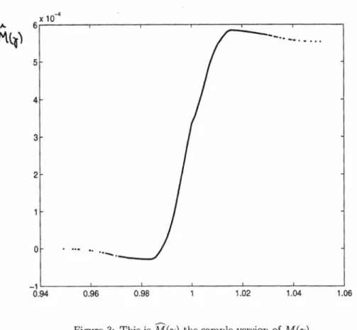
P ro p o s itio n IV : A sufficient c o n d itio n for (14) is t h a t E (R l+\) > 0 a n d 3 d s.t M(pi) > 0 V 7 a n d M (7) > 0 for a t le a s t one 7,w here:

M ( 7 ) =

P

Rt+idF(Rt+1) -

f

^ +1d G « , )

P ro o f

As is well known, the condition of Proposition IV is a sufficient condition for:

E lF (R t+1) > E U \R m ) V concave IP

Notice now th at when E (R l+1) > 0 then O' > 0 and so +

Q*x)) is also concave in x, since: & lP (W t(l +6»*x)) = W fi'U ' > 0

£ iU '( W t(l + P x ) ) = (Wt0*)2U" < 0 Therefore it must also be that

ElP(W t(l + r < , ) ) > ElP{Wt{l + 99R l+l))m

Hence, (14) can replaced with:

: 3 d s.t. f R t+1dF (R t+1) - f R^+,dG(R^+1) > 0 V7 (19) J —OO J —OO © The Author(s). European University Institute. version produced by the EUI Library in 2020. Available Open Access on Cadmus, European University Institute Research Repository.

(29)

and the inequality is strict for at least one 7

Whilst a formal statistical test of (16) is feasible, it is incredi bly cumbersome computationally (sec Tolley and Pope, 1988) especially when, as here, there are many observations on R t+i and R$+1. Here, we offer a casual evaluation of whether Ho can be rejected by inspecting a plot of the sample version of M (7) for the optimal moving average returns iZf+j.

Insert Figure 3 Here

Observing figure 3, we notice th at for small 7, M (7) < 0 . This in dicates th a t the minimum returns from the optimal trading rule resulted in smaller returns than the long position. Hence, for example, an agent with a minimax utility function would prefer n o t to u se the trading rule. Therefore, it is unlikely that can be rejected and thus we are unable to show that the use of trading rules or conditioning on past prices is utility increasing for all risk-averse agents.

5 .2 E fficien cy w ith T ra n sa c tio n C o sts

So far we have shown that without transaction costs, there existed an ar bitrage opportunity for agents in the DJIA index who had mean-variance utility. We now turn to see how the inclusion of transaction costs affect these results. First of all, transaction costs will alter the analysts’ learn ing problem; hence, we replace (8) with:

(n*,Â*) = arg max {EttJ _ TOM A (P (,n,A )H £+1

n € N,ACA

- c \ M A ( P u n , \ ) - M A (P i- 1,n,X )\} (20) c are proportional transaction costs

r - 1 BI57

And derive jd ( n £, A£) j and R£v,for various levels of c. Our

ob-© The Author(s). European University Institute. version produced by the EUI Library in 2020. Available Open Access on Cadmus, European University Institute Research Repository.

(30)

jective will be to determine the level of transaction costs21 c for which

Hq can be rejected in favour of / / ” “ at the 95% confidence level22.

In Table III below we have, amongst other tilings, tabulated the returns from a rule used by the analyst who solves (17). The level of costs at which Ho can be rejected under the assumption th a t R l+},B f+i ~ N

i.i.d. is represented by the line dividing Table III. Notice that this table

incorporates the special case c = 0, as described in Table II.

Rules Mean Return St. Dev. P r{R't < B t) n ? I f ( i + Rl) Market B,t 0.0002334 0.008459 - 2.378 Opt. TTR 1!

o

0.000801 0.008335 8.887e-05 110.7 c=0.0001 0.0007304 0.008328 0.0005109 71.41 c=0.0002 0.0006911 0.008321 0.001238 55.88 c=0.0003 0.0006196 0.008318 0.00533 35.63 c=0.0004 0.0005508 0.008311 0.01788 22.99 c=0.0005 0.0004893 0.008305 0.0452 15.44 c=0.0006 0.0004707 0.00829 0.058 13.67 c=0.0007 0.0003741 0.00828 0.1755 7.101 c—0.0008 0.0003099 0.008273 0.3061 4.456 c—0.0009 0.0002763 0.008205 0.3876 3.453

r—1

o o

o

IIo _0.0002191 _0.008215 _0.5379 _2.13

21Note that as defined, the cost of switching from a long to a short position and vice versa is 2c.

"It is important, to note that Proposition II can be extended to the case of trans action costs if these are small enough. The same is not true for Proposition I if trans action costs are proportional. For a more extensive discussion of technical analysis with transaction costs see Skouras, 1997.

(31)

T ab le III: The first column indicates which level of costs is

under consideration. The next two columns indicate the empirical mean and the standard deviation of the rules’ returns (note that Prop. II is confirmed). The fourth, column shows the probability (under the assumption of normal distributions) that the m.ean returns from a specific rule were smaller or equal to those of a non market timer. The final column shows the cumulative returns from each strategy during the whole time period.

The table indicates that at the 5% level of significance, LIA will be accepted for c > 0.06%. The mean return of the optimal rule remains larger for c < 0.09% (but not for the usual margin of confidence). Whilst these levels of c are probably high enough to guarantee that in today’s cost conditions LIA might be violated23, costs were certainly larger at the beginning of the sample we have considered. How large the decrease in transaction costs has been and how it has affected different types of investors is a question which is beyond the scope of this paper, so we do not attem pt to answer it. We must add the warning th a t the time-series used is not adjusted for dividends- and hence our results are likely to be biased against LIA.

6 C on clusion s

This paper has been organised around the objective of developing de finitions and assumptions which would allow technical analysis to be approached in a utility maximisation framework. Its starting point is the illustration th at technical analysis is consistent with expected util ity maximisation in a typical investment problem when preferences are risk-neutral.

Viewing technical analysis as the decision problem of an agent learn ing to maximise his expected utility, formalises the notion of ’optimal

23 An investor with access to a discount broker, c.g. via email, can purchase 1000 shares of a company listed on the NYSE for SM.95.

(32)

technical analysis’ hitherto loosely alluded to in various papers. The for malisation is revealing because it clearly illustrates th a t a rule can only be optimal with respect to a specific decision problem and hence a spe cific class of rules, a level of transaction costs, a position in the market and most importantly a utility function. This indicates th at a generally optimal technical analysis is a chimera and that when rules are chosen, it is useful to base this choice on an explicit criterion based on a decision problem.

In a more empirical vein, we show that using learned rules can lead to inferences winch are more powerful than those based on arbitrary rules as well as subject to fewer data-mining problems. Consequently, we suggest th a t model specification tests based on rule returns as pioneered by Brock et al. (1992) should be augmented by use of ’artificial’ technical analysts in the spirit of Sargent (1993).

Finally, we have tried to investigate the relationship between trad ing rule returns and market efficiency. This investigation has limited itself to developing and applying a way of empirically rejecting LI A, the hypothesis th a t past prices do not affect investment decisions. The con clusion drawn from our empirical test is th at if the DJIA is the only risky asset in an economy, the hypothesis can be rejected for agents with mean-variance utility facing low enough transaction costs; however, the same is not true for all risk-averse agents. We interpret the magnitude of transaction costs for which this hypothesis is rejected as a measure of market inefficiency.

Natural extensions of this work lie mainly in empirical applications of the developed framework. Firstly, further development of the idea that technical analysis is an effective form of prediction for certain types of loss functions is warranted, since it is likely th at this could lead to the development of useful classes of trading rules. Secondly, a more detailed application of the ’optimal’ rule to model specification tests could yield significant insights as to the nature of financial time-series. Finally, it is quite easy to extend the framework so as to allow the technical analyst to choose rules conditional on variables other than past prices. This indicates that, in principle, even fundamental analysis is not beyond the

(33)

scope of this ’theory of technical analysis’.

R eferen ces

[1] Allen F., Karjalainen It., 1996, ’Using Genetic Algorithms to find Tech nical Trading Rules’, working paper, University of Pennsylvania. [2] Allen P. M., Phang II. K., 1994, Managing Uncertainty in Complex Sys

tems: Financial Markets, in Evolutionary Economics and Chaos theory, in L. Leyesdorff, P. Van den Bessclaar,(eds) 1994, Evolutionary Economics and Chaos Theory, Pinter, London.

[3] Allen P. M., Phang K., 1993, Evolution, Creativity and Intelligence in Complex Systems, in II. Ilakcn and A. Mikhailov (eds.), Interdis ciplinary approaches to Nonlinear Complex Systems, Springer-Verlang, Berlin, 1993.

[4] Allen II, Taylor M. P.,(1990), ’’Charts, Noise and Fundamentals in the London Foreign Exchange Market”, Economic Journal, 100, pp.49-59 [5] Allen II.,Taylor M. P.(1989), The Use of Technical Analysis in the Foreign

Exchange market., Journal of International Money and Finance 11: 304- 314.

[0] Arthur W. B., 1992, ’On learning and adaptation in the economy’, Santa Fe Institute wp 92-07-038.

[7] Arthur W. B., Holland J. II., LeBaron 13., Palmer R., Tayler P., 1996, As set Pricing Under Endogenous expectations in an Artificial Stock Market, Santa Fe Institute working paper.

[8] Black, F., 1986, ’Noise’, Journal of Finance 41, 529-43.

[9] Blume L., Easley D., O’Hara M., 1994, Market Statistics and Technical Analysis: The role of Volume, Journal of Finance, Vol. XIIX, No. 1. [10] Brock W., Lakonishok .1., LeBaron B., 1991, Simple Technical Trading

Rules and the Stochastic properties of Stock Returns, Santa Fe Institute working paper. © The Author(s). European University Institute. version produced by the EUI Library in 2020. Available Open Access on Cadmus, European University Institute Research Repository.

(34)

[11] Brock W., Lakonishok J., LeBaron B., Simple Technical IVading Rules and the stochastic properties of Stock Returns, Journal of Finance, 47(5): 1731-1764.

[12] Chiang T. F., 1962, technical Trading Rules Based on Classifier Systems: A New Approach ro Learn from Experience, Unpublished Dissertation UCLA.

[13] Conroy R., Harris R., 1987, Consensus Forecasts of Corporate Earnings: Analysts’ Forecasts and Time Series Methods.” Management Science 33 (June 1987) :725-738.

[14] Christofferson F. F., Diebold F. X., (1995), ’Further results on Forecasting and Model Selection Under Asymmetric Loss’, Working Paper.

[15] Cumby R. E., D. M. Modest, 1987, ’Testing for Market Timing Ability: A framework for forecast evaluation’, Journal of Financial Economics 19, ppl69-189.

<

[16] Curcio R., Goodhart C., 1991, Chartism: A Controlled Experiment., Discussion Paper #124, Financial Markets Discussion Group Series, LSE. ,V [17] Faina E., 1991, Efficient Capital Markets: II, Journal of Finance, XLVL,

5, pp.1575-1617.

[18] Goldberg M. I)., Schulmeister S., (1989), ’’Technical Analysis and Stock Market Efficiency” , Discussion Papers...

[19] Hanoch G., Levy II., 1969, "The efficiency analysis of choices involving risk”, Review of Economic Studies, 36, 335-346.

[20] Jensen M., 1978., ’Some anomalous evidence regarding market efficiency’, Journal of Financial Economics 6(2-3), 107-147.

[21] Kandel S., Stambaugh R. F., 1996, ’On the predictability of stock returns: An asset-allocation perspective’, Journal of Finance, LI, 2.

[22] Kaufman, 1978, Commodity Trading Systems and Methods, John Wiley & Sons.

[23] Lakonishok J, Visliny R. W., Shleifer A, 1993, ’Contrarian Investment, Extrapolation and Risk’, NBER, wp 4360.

(35)

[2d] LeBaron B, 1991, ’Technical Trading rules and Regime shifts in Foreign Exchange’, SFI WP 91-10-044.

[25] LcBaron B, 1992, ’Do Moving Average 'Trading Rule Results Imply Non- linearities in the Foreign Exchange Markets?’, U. Wisconsin w.p.. [26] Leitch G. and J.E. Tanner, 1991, ’Economic Forecast Evaluation: Profits

Versus the Conventional Error Measures’, AER 81(3), pp. 580-590. [27] Levich R., and L. Thomas, 1993, ’The significance of technical-trading

rulles profits in the foreign exchange market: A bootstrap approach’, Journal of International Money and Finance, 56, 269-290.

[28] Markowitz, 1987, Mean Variance Analysis in Portfolio Choice and Capital Markets, McMillan.

[29] Malkicl B. G., 1992, ’Efficient Market Hypothesis’, in Eatwell J., Milgate M. and P. Newman (cds.), The New Palgrave Dictionary of Banking and Finance, McMillan.

[30] Malkiel B. G., 1996, A Random Walk Down Wall Street, , W. W. Norton & Company. Inc.

[31] Murphy J. J., 1986, Technical Analysis of the Futures Markets, New York: New York Institute of Finance.

[32] Neely C., Weller P., Dittmar R., 1996, ’Is Technical Analysis in the Foreign Exchange Market Profitable? A Genetic Programming Ap proach’,CEPR d.p. #1480.

[33] Neftci S. N., 1991, ’Naive Trading Rules in Financial Markets and Wicner- Kolmogorov Prediction Theory: A Study of ’Technical Analysis’ ’, Jour nal of Business, 64(4).

[34] Olsen R. B., M. M. Dacorogna, U. A. Muller, 0 . V. Pictet, 1992, ’Going Back to the Basics -Rethinking Market Efficiency’, O&A Research Group discussion paper.

[35] Pau L. F., 1991, Technical analysis for portfolio trading by symmetric pattern recognition, Journal of Economics Dynamics and Control, Journal of Economic Dynamics and Control 15, 715-730.

(36)

[36] Pictet, O. V., Dacorogna M. M., Dave 11. 1)., Ghopard IB., Schirru R., Tomassiiii M., 1996, ’Genetic Algorithms with collective sharing for ro bust optimization in financial applications’, Neural Network World, 5(4), pp.573-587.

[37] Ross, S.A., 1987, ’the Interrelations of Finance and Economics; Theoret ical Perspectives’, AER, 77(2), 29-34.

[38] Sargent T. J., 1993, Bounded Rationality in Macroeconics, Oxford: Clarc- don, Oxford University Press.

[39] Satchell S., Timmerman A., 1995, ” An Assesment of the Economic Value of Nonlinear Exchange Rate Forecasts” , WP UCSD, March 1995. [40] Skouras S., 1997, A Theory of Technical Analysis (Unabridged), Mimeo.,

European University Institute.

[41] Taylor S. J., 1994, ’Trading Futures using a channel rule: A study of the predictive power of technical analysis with currency examples’, Journal of Futures Markets, 14(2), pp.215-235.

[42] Teweles R.J., Harlow C.V., Stone II.L., 1977, The Commodity Futures Game, McGraw-Hill.

[43] Treynor J. L., Ferguson R., 1985, In Defence of Technical Analysis, Jour nal of Finance, XL, 3.

[44] Tolley H. D., Pope R. D., 1988, Testing for Stochastic Dominance, Journal of Agricultural Economics.

[45] White H, 1992, Artificial Neural Networks: Approximation and Learning Theory, Blackwell. © The Author(s). European University Institute. version produced by the EUI Library in 2020. Available Open Access on Cadmus, European University Institute Research Repository.