A new approach for the quantification of qualitative measures of economic expectations

1

A new approach for the quantification of qualitative measures of

economic expectations

Oscar Claveria¹*_{, Enric Monte², Salvador Torra³}

¹ AQR-IREA, University of Barcelona (UB)

² Department of Signal Theory and Communications, Polytechnic University of Catalunya (UPC) ³ Riskcenter-IREA, Department of Econometrics and Statistics, University of Barcelona (UB)

Abstract

In this study a new approach to quantify qualitative survey data about the direction of change is presented. We propose a data-driven procedure based on evolutionary computation that avoids making any assumption about agents’ expectations. The research focuses on experts’ expectations about the state of the economy from the World Economic Survey in twenty eight countries of the Organisation for Economic Co-operation and Development. The proposed method is used to transform qualitative responses into estimates of economic growth. In a first experiment, we combine agents’ expectations about the future to construct a leading indicator of economic activity. In a second experiment, agents’ judgements about the present are combined to generate a coincident indicator. Then, we use index tracking to derive the optimal combination of weights for both indicators that best replicates the evolution of economic activity in each country. Finally, we compute several accuracy measures to assess the performance of these estimates in tracking economic growth. The different results across countries have led us to use multidimensional scaling analysis in order to group all economies in four clusters according to their performance. We obtain the best results for Belgium, Norway, Austria, Lithuania, Japan and the United Kingdom.

Keywords

Economic growth; Qualitative survey data; Expectations; Symbolic regression; Evolutionary algorithms; Genetic programming

JEL Classification: C51; C55; C63; C83; C93

* _{Corresponding author. Tel.: +34-934021825; Fax.: +34-934021821. Department of Econometrics,} University of Barcelona, Diagonal 690, 08034 Barcelona, Spain. E-mail address: oclaveria@ub.edu

1 Introduction

Economic expectations about future economic conditions are a key feature in macroeconomic models. Qualitative survey data on the direction of change are one of the main sources of agents’ expectations. Tendency surveys ask respondents whether they expect a wide range of variables to rise, to fall, or to remain unchanged. Survey-based expectations present two main advantages over experimental expectations. Apart from being based on the knowledge of the respondents operating in the market, they are available ahead of the publication of quantitative official data, which makes them very useful for prediction. Additionally, survey data provide detailed information about different economic variables, ranging from capital expenditures and private consumption to exports and imports. This feature makes survey expectations especially indicated for the design of synthetic indicators.

One of the main drawbacks of survey-based expectations is their qualitative nature. With the aim of overcoming this limitation, numerous quantification methods have been proposed in the literature (Nardo, 2003; Driver and Urga, 2004; Pesaran and Weale, 2006; Vermeulen, 2014). This line of research centered in the conversion of qualitative responses about the expected direction of change into a quantitative measures has evolved in parallel with the application of new econometric techniques.

Recent developments in empirical modelling allow to generate mathematical models from a given dataset. Empirical modelling has two main advantages over conventional approaches. On the one hand, it is especially suitable for finding patterns in large data sets, where little or no information is known about the system. On the other hand, empirical modelling allows to simultaneously evolve both the structure and the parameters of the model.

In a recent study, Lahiri and Zhao (2015) examine the quality of quantified expectations by comparing them to quantitative realizations at the firm-level, obtaining significant improvements when relaxing the assumptions of quantification methods of qualitative survey data, particularly during periods of uncertainty, with high levels of disagreement between respondents.

These findings have led us to look for a data-driven assumption-free approach to transform survey measures of agents’ expectations into quantitative estimates. We aim to break new ground in the quantification of survey responses on the direction of change by

3 presenting a new method based on the implementation of recent developments in evolutionary computation to qualitative survey data.

The CESIfo Institute for Economic Research elaborates World Economic Survey (WES), which polls experts in 123 countries about economic trends (Kudymowa et al., 2013). We use twelve survey variables from the WES in twenty eight countries of the Organisation for Economic Co-operation and Development (OECD) to generate quantitative estimates of economic growth. In a first step, we combine and transform agents’ expectations about the future state of the economy. We repeat the experiment for agents’ judgements about the present state of the economy. As a result, we derive a leading indicator and a coincident indicator of economic activity. In a second step, we apply index tracking, which is a procedure used for portfolio management, to calculate the optimal relative weights of both indicators that best replicates the evolution of the Gross Domestic Product (GDP) in each country.

With the aim of examining the leading properties of these estimates of economic growth, we compute several accuracy measures to assess their predictive content and to evaluate their cyclical properties in terms of the level of synchronization with the quantitative variable of reference. Finally, by means of a dimensionality reduction technique, we synthesize all the information provided by these performance measures and the characteristics of the data into two factors that allow us to cluster all economies into four groups.

The structure of the paper is as follows. The next section reviews the existing literature. In Section 3 we present the methodological approach and describe the experiment. Empirical results are provided in Section 4. Finally, conclusions are given in Section 5.

2 Literature review

2.1 Quantification of qualitative survey data

The first attempt to quantify survey expectations is that of Anderson (1951, 1952), who proposed the balance statistic as a measure of the evolution of the quantitative variable it refers to. Aggregating individual replies as percentages of the respondents in each category, and assuming that the expected percentage change in a variable remains constant over time for all agents, the balance statistic is obtained as the subtraction between the percentage of agents reporting an increase and the percentage reporting a

decrease. Based on these premises, Pesaran (1984, 1985) developed this framework to allow for an asymmetrical relationship between individual changes and the evolution of the quantitative variable of reference. Using the relationship between actual values and respondents’ perceptions of the past as yardstick for the quantification of expectations about the future, the author proposed the regression approach.

By making positive and negative individual changes dependent on past values of the quantitative variable of reference, Smith and McAleer (1995) proposed a non-linear dynamic regression model to quantify survey responses that can be regarded as an extension of the regression approach. A drawback of the regression approach to quantify survey responses is that there is no empirical evidence that agents judge past values in the same way as they formulate expectations about the future (Nardo, 2003). As a result, the regression approach is restricted to expectations of variables over which agents have direct control, be it prices or production. The development of this approach has also been conditioned by the procurement of a rationale for the application, which can only be obtained by means of the analysis of individual data. For an an appraisal of individual firm data on expectations see Zimmermann (1997).

Theil (1952) designed a theoretical framework to generate quantitative estimates from the balance statistic proposed by Anderson (1951). Based on the assumption that respondents report a variable to go up (or down) if the mean of their subjective probability distribution lies above (or below) a certain level, the author defined the indifference threshold, also known as the difference limen. This threshold was conceived as an interval around zero within which respondents perceive there are no significant changes in the variable, and respond that the variable remains unchanged. Let yit indicate the percentage change of variable Yit for agent i from time t1 to time t, and Rt and Ft, denote the aggregate percentage of respondents at time t1 expecting a variable to rise or fall at time t respectively. If e

it

y is the unobservable expectation that agent i has over the change of variable Yit, the indifference interval can be defined as





it

b are the lower and upper limits of the indifference threshold for agent i regarding time

t. Assuming that response bounds are symmetric and fixed both across respondents and over time (ait bit  , i,t ), and that agents base their answer according to an independent subjective probability distribution that has the same form across respondents, the author generated quantitative estimates of yˆt.

5 Knöbl (1974) and Carlson and Parkin (1975) further developed the probability approach proposed by Theil (1952). As estimates of yˆt are conditional on a particular value for the imperceptibility parameter , and a specific form for the aggregate density function, Carlson and Parkin (1975) assumed that the individual density functions were normally distributed, and estimated  by assuming that over the sample-period yˆt is an unbiased estimate of yt . Consequently, the role of  is to scale the aggregate expectations e

t

y such that the average value of yt equals e t

y . Thus, using the evolution of the observed variable as a yardstick qualitative responses can be transformed into quantitative estimates.

Fishe and Lahiri (1981), Batchelor (1982), Visco (1984), and Foster and Gregory (1987) used alternative distributions. There is inconclusive evidence on the type of probability distribution aggregate average expectations come from. While Carlson (1975), Batchelor (1981), Batchelor and Dua (1987), Foster and Gregory (1987) and Lahiri and Teigland (1987) reject the hypothesis of normality, Dasgupta and Lahiri (1992), Balcombe (1996), Berk (1999) and Mitchell (2002) find evidence that normal distributions provide as accurate expectations as other non-normal distributions.

Another line of research has focused on refining the probability approach by relaxing the assumptions symmetry and constancy of the indifference bounds. Several strategies have been proposed in the literature in order to introduce dynamic imperceptibility parameters in the probability approach. Bennet (1984), Batchelor (1986), Kariya (1990), and Berk (1999) made the threshold dependent on time-varying quantitative variables. Batchelor and Orr (1988) imposed the unbiasedness condition over predefined subperiods. Mitchell et al. (2007) generalized the Carlson-Parkin procedure to generate cross-sectional and time-varying proxies of the variance.

Using a time-varying parameter model (Cooley and Prescott, 1976) together with the Kalman filter (Kalman, 1960) for parameter estimation, Seitz (1988) was able to simultaneously introduce asymmetric and time-varying indifference thresholds. The author assumed that the imperceptibility parameters were subject to permanent and temporary shocks. Claveria et al. (2007) extended this framework by using a state-space representation that allowed for asymmetric and dynamic response thresholds generated by a first-order Markov process.

Further improvements of quantification procedures have been developed at the micro level, either by means of experimental expectations generated by Monte Carlo simulations, or by comparing the individual responses with firm-by-firm realisations.

Regarding the former option, Common (1985) generated simulated expectations to test the rational expectations hypothesis. Nardo and Cabeza-Gutés (1999) designed a simulation experiment to assess the performance of the different quantification methods. By means of simulation-based expectations, Löffler (1999) and Terai (2009) estimated the measurement error introduced by the probabilistic method. Additionally, Löffler (1999) proposed a refinement of the Carlson-Parkin method. Claveria (2010) used computer-generated expectations to assess the forecasting performance of different quantification methods, and presented a variation of the balance statistic that took into account the proportion of respondents reporting that the variable remains unchanged.

Using firm-level survey responses, Mitchell et al. (2002) developed a procedure to quantify individual categorical expectations based on the assumption that responses are triggered by a latent continuous random variable as it crosses time-varying thresholds, and found evidence against time invariant thresholds. By introducing the “conditional absolute null” property, based on the empirical finding that the median of realized quantitative values corresponding to the “no change” category is zero, Müller (2010) proposed a variant of the Carlson-Parkin method with asymmetric and time invariant thresholds, which allows to solve the zero response problem that occurs when all respondents fall into one of the extreme responses (an increase or a decrease).

The variation of the indifference thresholds across individuals can only be tested by means of the analysis of individual expectations. Using a matched sample of qualitative and quantitative individual stock market forecasts, Breitung and Schmeling (2013) corroborated the importance of introducing asymmetric and dynamic indifference parameters, but found that individual heterogeneity across respondents plays a minor role in forecast accuracy. On the other hand, Lahiri and Zhao (2015) have recently found strong evidence against the threshold constancy, symmetry, homogeneity, and overall unbiasedness assumptions of the probability method. The authors have generalized the Carlson-Parkin framework by means of a hierarchical ordered probit model. Based on a matched sample of households, they have found that when the unbiasedness assumption is replaced by a time-varying calibration, the resulting quantified series is found to better track the quantitative benchmark.

2.2 Evolutionary computation

Evolutionary computation is a subfield of artificial intelligence that is increasingly being applied in economics in the context of expensive optimization. Evolutionary computation

7 is based on the implementation of algorithms that adopt Darwinian principles of the theory of natural selection to automated problem solving. These algorithms are known as evolutionary algorithms (EAs). Evolutionary programming was introduced by Fogel et al. (1966). The most popular type of EA is the genetic algorithm (GA), which was initially proposed by Holland (1975). Cramer (1985) developed a generalization of GAs known as genetic programming (GP). GP is a soft-computing search technique that allows the model structure to vary during the evolution, which makes it particularly indicated for non-linear and empirical modelling. See Poli et al. (2010) for a review of the state of the art in GP.

Chen and Kuo (2002) classified the literature on the application of evolutionary computation to economics and finance. Most evolutionary computing in economics has been implemented in finance (Goldberg, 1989). On the one hand, with respect to GAs, Acosta-González and Fernández (2014) used a GA to predict the financial failure of firms, and Acosta-González et al. (2012) to explain the 2008 financial crisis. Lawrenz and Westerhoff (2003) modelled exchange rates with a GA. Maschek (2010) evaluated the performance of the self-adaptation mechanism in GAs for the convergence to the rational expectations equilibrium. Thinyane and Millin (2011) applied GAs to optimize the signals generated by technical trading tools. Vasilakis et al. (2013) presented a GP-based technique to predict returns in the trading of the euro/dollar exchange rate. Wei (2013) used an adaptive expectation GA to optimize a fuzzy model to forecast stock price trends in Taiwan. For a review of the applications of GAs for financial forecasting see Drake and Marks (2002).

On the other hand, regarding GP, Álvarez-Díaz and Álvarez (2005) applied GP to predict exchange rates. Chen et al. (2008) analysed the performance of GP to financial trading. Kaboudan (2000), Larkin and Ryan (2008), and Wilson and Banzhaf (2009) used GP for stock price forecasting. Yu et al. (2004) implemented a GP approach to model short-term capital flows.

Applications of GP in macroeconomics have been very limited. The first application of GP is that of Koza (1992), who used GP to reassess the exchange equation relating the price level, gross national product, money supply, and the velocity of money. Chen et al. (2010) applied GP in a vector error correction model for macroeconomic forecasting. Duda and Szydło (2011) developed economic forecasting models by means of gene expression programming (GEP), which can be regarded as a version of GP (Ferreria, 2011).

Koza (1992) developed GP to find the best single computer program to implement symbolic regression (SR). SR can be regarded as a new approach to empirical modelling. Given a predetermined set of operations and functions, SR searches appropriate models from the space of all possible mathematical expressions that best fit the data. Zelinka (2005) introduced analytical programming in order to synthesize suitable solutions in SR. Due to its versatility, SR is being increasingly used in different areas: from industrial data analysis (Vladislavleva et al., 2010) and the experimental design of manufacturing systems (Can and Heavey, 2011), to signal processing (Yao and Lin, 2009) and other various applications (Barmpalexis et al., 2011; Cai et al., 2006; Ceperic et al., 2014; Sarradj and Geyer, 2014; Wu et al., 2008).

There have been very few applications in macroeconomics. Claveria et al. (2016) implemented SR via GP to derive a set of building blocks used with forecasting purposes. Kľúčik (2012) applied SR to estimate total exports and imports to Slovakia. Kotanchek et al. (2010) used SR via GP for GDP forecasting. By means of SR, Kronberger et al. (2011) identified interactions between economic indicators in order to estimate the evolution of prices in the US. Yang et al. (2015) used SR for production forecasting of crude oil. Recently, Peng et al. (2014) have proposed an improved GEP algorithm especially suitable for dealing with SR problems.

3 Data and methods

3.1 Data

This study matches two sources of information for twenty eight countries of the OECD: Austria, Belgium, Bulgaria, Croatia, the Czech Republic, Denmark, Estonia, Finland, France, Germany, Greece, Hungary, Ireland, Italy, Japan, Latvia, Lithuania, the Netherlands, Norway, Poland, Portugal, Romania, the Slovak Republic, Slovenia, Spain, Sweden, the United Kingdom (UK), and the United States (US). On the one hand, we use quantitative official statistics about the evolution of economic activity. Specifically, the year-on-year growth rates of quarterly GDP data from the OECD

(https://data.oecd.org/gdp/quarterly-gdp.htm#indicator-chart). The sample period goes

from the third quarter of 2000 to the first quarter of 2014. On the other hand, we use qualitative survey data reflecting agents’ expectations about the future, and their judgements about the present economic situation.

9 We focus on the main survey variables from the the WES, which assesses worldwide economic trends by polling professionals and experts on current economic developments in their respective countries (Kudymowa et al., 2013). Białowolski (2016) notes that professional respondents are characterized by significantly lower biases in responding to survey questions than consumers. Franses et al. (2011) also find evidence in favor of experts’ forecasts when compared with pure model forecasts. See Henzel and Wollmershäuser (2005), Stangl (2007), and Hutson et al. (2014) for an appraisal of the WES.

Respondents are asked about the economic situation in three different forms: their expectation by the end of the next six months (variables X7 to X12), their present judgement (variables X1 to X3), and their assessment compared to the same time last year (variables X4 to X6). The economic situation is assessed with respect of three items: the overall economy (variables X1, X4 and X7), capital expenditures (variables

2

X , X5 and X8), and private consumption (variables X3, X6 and X9). Respondents are also asked about their expectations about the volume of exports (X10), of imports (X11), and the balance of trade (X12). All twelve variables are presented in Table 1.

Table 1 World Economic Survey (WES) – Survey indicators

Present Compared to last year For the next six months Economic situation Economic situation Economic situation and

foreign trade volume 1

X overall economy X4 overall economy X7 overall economy 2

X capital expenditures X5 capital expenditures X8 capital expenditures

3

X private consumption X6 private consumption X9 private consumption 10 X volume of exports 11 X volume of imports 12 X balance of trade

In order to present the survey results, the Ifo uses a grading procedure which is conceptually equal to calculating balances: positive replies are assigned a grade of nine; indifferent replies, of five; and negative replies, of one. Country results are weighted according its share of exports and imports in total world trade (CESifo World Economic Survey, 2016). The Ifo also constructs an aggregate indicator obtained as the arithmetic mean of assessments of the general economic situation and the expectations for the economic situation in the next six months: the Economic Climate Indicator (ECI). The ECI tends to correlate closely with the actual business-cycle trend measured in annual growth rates of real GDP (Claveria et al., 2016; Garnitz et al., 2015).

3.2 Methods

SR is based the search of relationships between a given set of variables. The major difference in relation to conventional regression analysis resides in the fact that while the former is based on a certain model specification, SR does not rely on a specific a priori determined model structure. The only assumption made in SR is that the response surface can be described by an algebraic expression.

GP can be regarded as an extension of GAs in which the solutions are expressed in the form of computer programs. The main difference between them is in the representation of the structure: while GP codes potential solutions by means tree-structured, variable length representations, GAs use fixed length binary string representations. GP’s more general representation scheme allows the model structure to vary during the evolution. This feature is particularly suitable in the current study, where the functional relationship between the set of survey variables is arbitrary and unknown. Consequently, we use GP to solve the SR experiment, and to transform qualitative survey data into quantitative estimates of economic activity, formalizing the interactions between a wide range of survey-based indicators. The implementation of GP for SR was based on the following sequence of steps:

First – The creation of an initial population. We determined a population size of 3 million individuals.

Second – Determination of a fitness function. In order to evaluate the fitness of each member of the population we use the Root Mean Square Error (RMSE).

Third – Determination of a strategy for the selection of parents for replacement. In order to guarantee the diversity in the population we use the tournament method.

Fourth – Determination of the probability of a new generation and application of genetic operators to the parents. The main genetic operations are reproduction (copy), crossover (recombination of randomly chosen parts of parents), and mutation (random alteration of a part of a parent). We select a 0.1 mutation probability to prevent trapping into local optima.

Fifth – Determination of constants. With the aim of avoiding the search path to deviate from the optimum we include the automatic generation of constants provided by the algorithm, which are optimized after a number of generations according to their correlation relative to the functional form.

11 Sixth – Determination of a stopping criterion. We set a maximum number of 150 generations as the termination criterion. Steps three and four are repeated until a new generation is created. If no individual in the population has a required minimal fitness, or the stopping criterion is fulfilled, everything is repeated using the new generation as the population. As a result, the fitness of the population is ever increasing.

The search process is characterized by a trade-off between accuracy and simplicity. To limit the complexity of the resulting expressions, the set of functions is restricted to some elementary functions. We use the Distributed Evolutionary Algorithms Package (DEAP) framework implemented in Python (Fortin et al., 2012; Gong et al., 2015).

By matching qualitative survey indicators from the WES to quantitative official data in two successive SR experiments, we are able to derive two analytical expressions: one linking agents’ expectations about the future (variables X7 to X12) to economic growth, and another one combining agents’ judgements about the present (variables X1 to X6).

4 Results

First, we present the output of the two SR experiments undertaken. On the one hand, expression (1), which combines agents’ expectations about the future, and can therefore be regarded as a leading indicator of economic activity ( yˆ1,it). On the other hand, expression (2), which combines agents’ judgements about the present state of the economy, and can be seen as a coincident indicator (yˆ_2,it):

              it it it it it it t i it X X X X X X X y 9 10 4 10 7 12 3 log 12 10 22 12 ˆ1, , (1)









Where the sub index i refers to each specific country at time t . In Fig. 1 we graphically compare the evolution of the two SR-generated indicators to that of the GDP. We can observe that while yˆ2,it is closely correlated to the oscillations of GDP in all countries, yˆ1,it shows a worse performance, especially since the 2008 financial crisis. Łyziak and Mackiewicz-Łyziak (2014) found that the 2008 financial crisis period had led to a decrease in expectational errors in transition economies. Claveria et al. (2016) obtained a similar result for ten Eastern European countries.

Fig. 1 Evolution of year-on-year GDP growth rates vs. survey-based economic indicators

Austria Belgium

Bulgaria Croatia

Czech Republic Denmark

Estonia Finland

France Germany

Note: The black dotted line represents the year-on-year growth rate of GDP in each country. The grey line represents the evolution of the proposed leading indicator. The black line represents the evolution of the proposed coincident indicator.

13

Fig. 1 (cont. 1) Evolution of year-on-year GDP growth rates vs. survey-based indicators

Greece Hungary

Ireland Italy

Japan Latvia

Lithuania Netherlands

Norway Poland

Note: The black dotted line represents the year-on-year growth rate of GDP in each country. The grey line represents the evolution of the proposed leading indicator. The black line represents the evolution of the proposed coincident indicator.

Fig. 1 (cont. 2) Evolution of year-on-year GDP growth rates vs. survey-based indicators

Portugal Romania

Slovak Republic Slovenia

Spain Sweden

United Kingdom United States

Note: The black dotted line represents the year-on-year growth rate of GDP in each country. The grey line represents the evolution of the proposed leading indicator. The black line represents the evolution of the proposed coincident indicator.

In a second step, we derive estimates of economic growth by combining the information of both indicators. We use a procedure of constrained optimization known as index tracking, which is used in finance in order to replicate the performance of stock indexes (Karlow, 2012; Kwiatkowski, 1992; Rudd, 1980). Index tracking consists on the minimization of a tracking error, defined as the expected squared deviation of return from

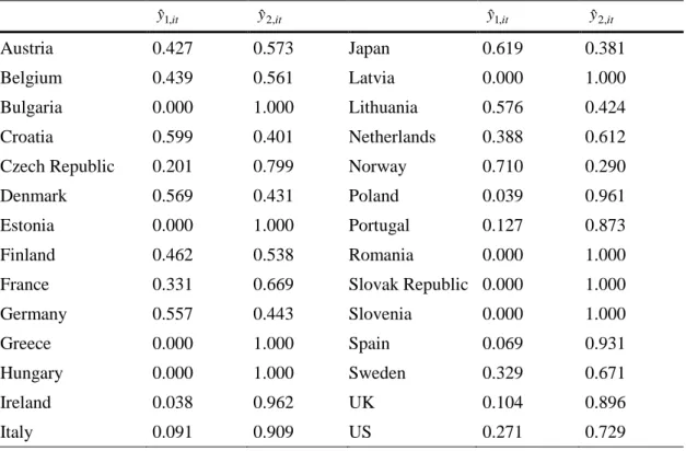
15 that of the index, with the aim of obtaining the proportion of capital to be invested in each asset. Based on this premise, we use a generalized reduced gradient algorithm to minimize the summation of squared forecast errors. We impose two restrictions in the optimization process with respect to the value of the weights. First, the sum of both weights must equal one. Second, the non-negativity restriction, so that the weights must be equal or larger than zero. As a result, we obtain the optimal weights of both the leading and the coincident indicator for each country (Table 2).

Table 2 Relative weights indicators – 28 OECD countries it yˆ1, yˆ2,it yˆ1,it yˆ2,it Austria 0.427 0.573 Japan 0.619 0.381 Belgium 0.439 0.561 Latvia 0.000 1.000 Bulgaria 0.000 1.000 Lithuania 0.576 0.424 Croatia 0.599 0.401 Netherlands 0.388 0.612

Czech Republic 0.201 0.799 Norway 0.710 0.290

Denmark 0.569 0.431 Poland 0.039 0.961

Estonia 0.000 1.000 Portugal 0.127 0.873

Finland 0.462 0.538 Romania 0.000 1.000

France 0.331 0.669 Slovak Republic 0.000 1.000

Germany 0.557 0.443 Slovenia 0.000 1.000

Greece 0.000 1.000 Spain 0.069 0.931

Hungary 0.000 1.000 Sweden 0.329 0.671

Ireland 0.038 0.962 UK 0.104 0.896

Italy 0.091 0.909 US 0.271 0.729

While the obtained relative weight of the coincident indicator is higher than that of the leading indicator, we observe numerous differences across countries. In Greece, Hungary, Latvia, Romania, the Slovak Republic, and Slovenia, the algorithm yields a null weight to the leading indicator constructed with agents’ expectations about the future. This result contrasts with that of Lacová and Král (2015), who found that in Slovakia companies are slightly more forward-looking than backward-looking. On the other extreme, in countries such as Norway and Japan, future expectations outweigh judgements about the present. This result brings up the question of whether survey-based indicators shall equally weight the information regarding the expectations about the future and the judgements about the present in all countries.

In the literature there is no consensus on the information content of survey expectations. Breitung and Schmeling (2013) compared quantified stock market

expectations with quantitative forecasts, and found that there was a weak correlation between them. Lacová and Král (2015) found that quantified survey expectations in Slovakia systematically failed to capture changes in consumer price index. Jonsson and Österholm (2011, 2012), Lui et al. (2011a,b) and Maag (2009) reached similar conclusions. On the other hand, there is ample evidence that survey expectations provide useful information for economic modelling (Altug and Çakmakli, 2016; Batchelor and Dua, 1992, 1998; Dees and Brinca, 2013; Girardi, 2014; Hansson et al., 2005; Jean-Baptiste, 2012; Klein and Özmucur, 2010; Leduc and Sill, 2013; Lemmens et al., 2005; Müller, 2009; Qiao et al., 2009; Schmeling and Schrimpf, 2011).

In order to evaluate the performance of the resulting estimates in monitoring economic activity, we compute several measures of forecast accuracy: the the mean absolute error (MAE) and the RMSE to assess the predictive content in terms of forecast accuracy, the mean absolute scaled error (MASE) to compare the forecasting performance to a benchmark model, and the Concordance Index (CI) proposed by Harding and Pagan (2002) to evaluate the cyclical properties in terms of the level of synchronization with the quantitative benchmark variable.

In Table 3 we present the MAE and the RMSE. We observe differences across countries. Austria, Belgium, Bulgaria, Estonia, and Lithuania present the lowest MAE and RMSE values. On the other extreme, Croatia, Hungary, Ireland, Italy and Poland are the economies where we obtain the least accurate predictions.

Table 3 Forecast accuracy – MAE and RMSE

MAE RMSE MAE RMSE

Austria 0.926 1.266 Japan 1.506 2.169

Belgium 0.978 1.187 Latvia 1.105 1.384

Bulgaria 0.889 1.190 Lithuania 0.824 1.012

Croatia 3.076 3.729 Netherlands 1.469 1.753

Czech Republic 1.816 2.324 Norway 1.290 1.770

Denmark 2.628 3.073 Poland 4.333 5.789

Estonia 0.910 1.154 Portugal 2.284 2.850

Finland 2.849 3.427 Romania 2.725 3.281

France 1.499 1.794 Slovak Republic 1.536 1.934

Germany 2.365 2.806 Slovenia 2.651 3.401

Greece 1.678 2.047 Spain 1.899 2.411

Hungary 5.546 6.631 Sweden 2.727 3.038

Ireland 3.075 4.379 UK 1.090 1.450

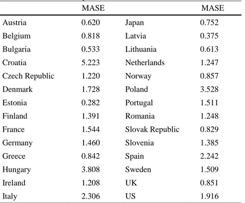
17 Next, we complement the assessment of the estimates by comparing them to those obtained with a benchmark model. With this aim, we compute the mean absolute scaled error (MASE) proposed by Hyndman and Koehler (2006). The idea behind the MASE is to scale the errors by the mean absolute errors obtained with a benchmark model. The MASE statistic presents several advantages over other forecast accuracy measures, as it is independent of the scale of the data, and it does not suffer from some of the problems presented by other relative measures of forecast accuracy (Hyndman and Koehler, 2006). An additional advantage is its easy interpretation, as values less than one indicate that the average prediction computed with the benchmark model is worse than the estimates obtained with the proposed method. If we denote e_t as the forecast error, the MASE can

be obtained as the mean of the absolute value of the scaled error q_t:

 

Given that official data are published with a delay of more than a quarter with respect to survey data, we use two-step ahead naïve forecasts as a benchmark. In Table 4 we present the MASE results. In Austria, Belgium, Bulgaria, Estonia, Greece, Japan, Latvia, Lithuania, Norway, the Slovak Republic and the UK, the estimates of GDP obtained with the proposed method outperform those of the benchmark model.

Table 4 Forecast accuracy – MASE

MASE MASE

Austria 0.620 Japan 0.752

Belgium 0.818 Latvia 0.375

Bulgaria 0.533 Lithuania 0.613

Croatia 5.223 Netherlands 1.247

Czech Republic 1.220 Norway 0.857

Denmark 1.728 Poland 3.528

Estonia 0.282 Portugal 1.511

Finland 1.391 Romania 1.248

France 1.544 Slovak Republic 0.829

Germany 1.460 Slovenia 1.385

Greece 0.842 Spain 2.242

Hungary 3.808 Sweden 1.509

Ireland 1.208 UK 0.851

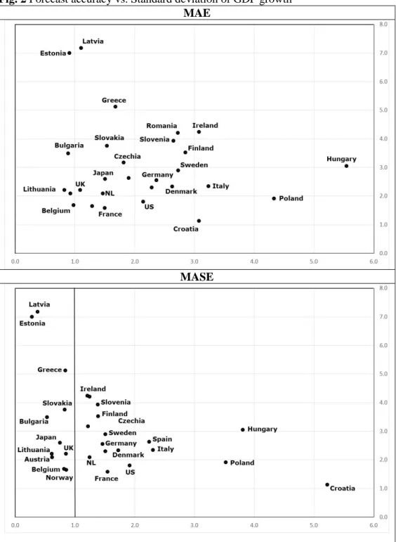
In Fig. 2 we compare the obtained forecast results to the standard deviation of the year-on-year growth rates of GDP. There seems to be no relation between neither the MAE or the MASE results and the the variability of economic activity. While Estonia and Latvia are the countries that present the highest levels of dispersion, the forecast errors are low, and the opposite holds for Croatia and Poland.

Fig. 2 Forecast accuracy vs. Standard deviation of GDP growth MAE

MASE

19 As there is evidence that the trend in the Ifo’s ECI correlates closely with the actual business-cycle trend measured in annual growth rates of real GDP (CESifo World Economic Survey, 2016), next we evaluate the cyclical properties of the proposed SR-generated estimates. We compare it with the ECI in terms of the level of synchronization. To that end, we use the Concordance Index (CI) proposed by Harding and Pagan (2002):







Where T is the number of observations, yt refers to the percentage growth rate of GDP and x_t to the variable under analysis. S is a binary variable that takes value one if the series is in expansion, and zero otherwise. As the C index developed by Harrell et al. (1996), the CI is expressed as the proportion of sample periods in which the two series are in the same phase of the cycle. Thus, the CI allows us to assess the proposed indicator in terms of regime shifts.

Table 5 Concordance Index – SR estimates vs. ECI

CI SR estimates ECI SR estimates ECI Austria 0.611 0.630 Japan 0.685 0.759 Belgium 0.741 0.667 Latvia 0.537 0.500 Bulgaria 0.500 0.537 Lithuania 0.407 0.426 Croatia 0.444 0.556 Netherlands 0.722 0.630

Czech Republic 0.593 0.574 Norway 0.556 0.667

Denmark 0.667 0.630 Poland 0.593 0.556

Estonia 0.630 0.611 Portugal 0.685 0.648

Finland 0.648 0.593 Romania 0.611 0.574

France 0.630 0.667 Slovak Republic 0.556 0.537

Germany 0.685 0.685 Slovenia 0.667 0.667

Greece 0.556 0.519 Spain 0.722 0.593

Hungary 0.574 0.463 Sweden 0.611 0.685

Ireland 0.630 0.611 UK 0.463 0.500

Italy 0.630 0.611 US 0.667 0.630

Notes: CI stands for concordance index (Harding and Pagan, 2002). A one value indicates that the cycles of the variables under comparison are in the same phase one hundred percent of times.

Results in Table 5 show that in most cases there are no major differences in CI values between both proxies. While in countries like Belgium, Finland, Hungary, the Netherlands, and Spain, the ECI shows a lower level of synchronization, the opposite holds for Japan and Norway.

To synthesize all the information provided by the above performance measures and the characteristics of the data, we finally compute two factors that allow us to cluster all economies into four groups. By transforming the original set of correlated performance measures into a smaller and more understandable set of uncorrelated factors, we aim to summarize the results of the present study. We make use of multidimensional scaling (MDS) analysis to generate a two-dimensional perceptual map in which we position all twenty eight economies according to their coordinates regarding the two factors. MDS is a multivariate analytical procedure also known as Principal Coordinates Analysis (Torgerson, 1952, 1958). For a detailed description of this technique see Hair et al. (2009) and Jolliffe (2002). MDS allows to visualize the level of similarity of individual cases of a dataset. In our case, the proximity between the different countries in the perceptual map indicates how similar they are in terms of the performance of survey-based measures of economic expectations.

First, we rank all twenty-eight countries in decreasing order according to their performance experienced over the sample period for each of the following measures: the weight of the leading indicator (yˆ1,_it ), the summation of squared forecast errors (SSE),

the MAE, the RMSE, the MASE, the CI, and the standard deviation of GDP growth (y_t )

in each country. Second, we assign a numerical value to each country corresponding to its position. We use the eigenvalues of the correlation matrix to generate a screeplot (Fig. 3) in order to identify the last component that accounts for a considerable amount of variance in the data, and therefore determine the number of dimensions. As we can see, the elbow is located at the third component, where there is a noticeable difference in slopes, indicating that the optimal number of dimensions is two.

21 After deciding on the number of components, we reduce the information of all rankings into two dimensions, which can be regarded as two synthetic indicators that maintain the original ordinal structures. We obtain a Kruskal stress value of 0.012, which indicates the amount of distortion in distances to tolerate. Stress values range from zero to one, where zero denotes a perfect representation of the input data in two dimensions. The two-dimensional scatterplot that represent the coordinates of the first two dimensions for each country is presented in Fig. 4.

Fig. 4 MDS Perceptual Map

The perceptual map is divided in four quadrants. In the top right quadrant, we find the countries with the highest scores in the two dimensions: Belgium, Norway, Austria, Lithuania, Japan and the UK. In this group of economies, the evolution of GDP displays a stable pattern, and expectations show a good forecasting performance. On the other extreme, in the lower left quadrant, we find the economies with the lowest scores in both dimensions: Ireland, Hungary, Slovenia, Poland, Italy, Finland, Sweden and Denmark, which is very close to Spain, Portugal and Germany in top left quadrant. Croatia is grouped apart, obtaining the lowest score in the first dimension, as opposed to Bulgaria, Estonia and Latvia, which are the economies with the highest scores in the first dimension.

According to Lee (1994), the differences between the actual values of a variable and quantified expectations may arise from three different sources: the measurement or conversion error due to the use of quantification methods to approximate unobservable expectations; the expectational error due to the agents’ limited ability to predict the movements of the actual variable; and the sampling errors. The groupings in Fig. 4 are indicative of different values regarding these three sources of error.

Finally, by means of an analysis of the variance (ANOVA) we test whether significant differences exist between the mean of each item across the four groups (Table 6). With the exception of the ranking regarding the CI, we find significant differences across clusters with respect to the mean of each of the performance measures used in the MDS analysis. These results suggest that the quantification of survey measures of expectations could be improved by adapting quantification procedures for countries with similar characteristics.

Table 6 ANOVA – Clusters MDS analysis

it

yˆ1,

 _{SSE MAE RMSE MASE CI}

t y  Cluster I Mean 6.667 11.833 5.833 6.333 7.167 16.167 8.000 Std. Dev. 5.574 6.113 3.430 4.320 2.787 11.197 4.382 Cluster II Mean 10.86 5.43 15.71 15.57 21.14 9.00 8.14 Std. Dev. 5.146 4.117 5.345 5.563 4.488 8.679 5.815 Cluster III Mean 16.50 16.38 23.63 23.63 20.50 13.50 16.88 Std. Dev. 8.018 5.097 3.249 3.249 5.372 4.928 6.312 Cluster IV Mean 22.57 23.71 10.29 10.00 7.29 19.71 23.71 Std. Dev. 4.353 4.386 6.726 6.557 5.499 5.024 3.498 ANOVA F statistic 8.649 16.948 17.394 15.924 18.911 2.438 14.446

p-value 0.000 0.000 0.000 0.000 0.000 0.089 0.000 Notes: ANOVA stands for analysis of variance to test whether a significant relation exists between the mean of each item across the four groups.

5 Conclusion

This paper proposes an empirical approach to transform qualitative survey responses on the direction of change into quantitative estimates of economic activity by means of symbolic regression via genetic programming. We used survey-based agents’ expectations about the economic situation from the World Economic Survey in twenty-eight countries of the OECD to derive a leading indicator, which consists of an optimal

23 combination of survey variables that best tracks the evolution of the economic activity. We repeated the experiment using agents’ perceptions about the present economic situation to obtain a coincident indicator.

We then combined the information from the leading and the coincident indicator by means of index tracking, which is a procedure to find the optimal relative weights of both indicators. By doing so, we generated quantitative proxies of economic activity. To assess the forecasting performance of the generated estimates, we computed several stylized facts and compared them to a benchmark model and to the Economic Climate Index constructed by the IFO. The heterogeneity of the results across countries led us to synthesize the information provided by all the forecast accuracy measures by means of a dimensionality reduction technique that allows us to cluster all economies according to their performance.

We obtained significant differences between mean values of each cluster, which indicates that the forecasting performance of survey-based expectations could be improved by designing ad-hoc quantification procedures for countries with similar characteristics.

Due to the novelty of the proposed approach, there are still several limitations to be addressed. Given that we used a data-driven method, the obtained quantitative estimates lack any theoretical background. Extending the analysis to other questionnaires would allow us to examine to what extent the obtained functional forms are extensive to different survey data. Another issue left for further research is assessing the effect of GDP updates on the results. Finally, there is the question of whether the implementation of alternative evolutionary algorithms could improve the forecast accuracy of empirically-generated quantitative estimates of expectations.

Acknowledgements

This paper has been partially supported by the Spanish Ministry of Economy and Competitiveness (TEC2015-69266-P). We also wish to thank Johanna Garnitz and Klaus Wohlrabe at the Ifo Institute for Economic Research in Munich for providing us the data used in the study.

References

Altug, S. and Çakmakli, C. (2016). Forecasting inflation using survey expectations and target inflation: Evidence from Brazil and Turkey. International Journal of Forecasting 32(1): 138–153.

Acosta-González, E., and Fernández, F. (2014). Forecasting financial failure of firms via genetic algorithms. Computational Economics 43(2): 133–157.

Acosta-González, E., Fernández, F., and Sosvilla, S. (2012). On factors explaining the 2008 financial crisis. Economics Letters 115(2): 215–217.

Álvarez-Díaz, M., and Álvarez, A. (2005). Genetic multi-model composite forecast for non-linear prediction of exchange rates. Empirical Economics 30(3): 643–663.

Anderson, O. (1951). Konjunkturtest und Statistik. Allgemeines Statistical Archives 35: 209–20. Anderson, O. (1952). The Business Test of the IFO-Institute for Economic Research, Munich,

and its theoretical model. Revue de l’Institut International de Statistique 20: 1–17. Balcombe, K. (1996). The Carlson-Parkin method applied to NZ price expectations using

QSBO survey data. Economics Letters 51(1): 51–57.

Barmpalexis, P., Kachrimanis, K., Tsakonas, A., and Georgarakis, E. (2011). Symbolic regression via genetic programming in the optimization of a controlled release

pharmaceutical formulation. Chemometrics and Intelligent Laboratory Systems 107(1): 75–82.

Batchelor, R. A. (1981). Aggregate expectations under the stable laws. Journal of Econometrics 16(2): 199–210.

Batchelor, R. A. (1982). Expectations, output and inflation: The European experience. European Economic Review 17(1): 1–25.

Batchelor, R. A. (1986). Quantitative v. qualitative measures of inflation expectations. Oxford Bulletin of Economics and Statistics 48(2): 99–120.

Batchelor, R. and Dua, P. (1987). The accuracy and rationality of UK inflation expectations. Applied Economics 19(6): 819–828.

Batchelor, R. and Dua, P. (1992). Survey expectations in the time series consumption function. The Review of Economics and Statistics 74(4): 598–606.

Batchelor, R. and Dua, P. (1998). Improving macro-economic forecasts. International Journal of Forecasting 14(1): 71–81.

Batchelor, R. and Orr, A. B. (1988). Inflation expectations revisited. Economica 55(2019): 317– 331.

Bennett, A. (1984). Output expectations of manufacturing industry. Applied Economics 16(6): 869–879.

Bergström, R. (1995). The relationship between manufacturing production and different business survey series in Sweden 1968-1992. International Journal of Forecasting 11(3): 379–393. Berk, J. M. (1999). Measuring inflation expectations: A survey data approach. Applied

Economics 31(11): 1467–1480.

Białowolski, P. (2016). The influence of negative response style on survey-based household inflation expectations. Quality & Quantity 50(2): 509–528.

Breitung, J. and Schmeling, M. (2013). Quantifying survey expectations: What’s wrong with the probability approach? International Journal of Forecasting 29(1): 142–154.

Cai, W., Pacheco-Vega, A., Sen, M. and Yang, K. T. (2006). Heat transfer correlations by symbolic regression. International Journal of Heat and Mass Transfer 49(23-24): 4352– 4359.

Can, B. and Heavey, C. (2011). Comparison of Experimental Designs for Simulation-based Symbolic Regression of Manufacturing Systems. Computers & Industrial Engineering 61(3): 447–462.

Carlson, J.A. (1975). Are price expectations normally distributed? Journal of the American Statistical Association 70(352): 749–754.

Carlson, J. A. and Parkin, M. (1975). Inflation expectations. Economica 42(166): 123–138. Ceperic, V., Bako, N. and Baric, A. (2014). A symbolic regression-based modelling strategy of

AC/DC rectifiers for RFID applications. Expert Systems with Applications 41(16): 7061– 7067.

CESifo World Economic Survey (2016). Vol. 15(2), May 2016.

Chen, X., Pang, Y. and Zheng, G. (2010). Macroeconomic forecasting using GP based vector error correction model. In J. Wang (Ed.), Business Intelligence in Economic Forecasting: Technologies and Techniques (pp. 1–15). Hershey, PA: IGI Global.

25 Chen, S. H. and Kuo, T. W. (2002). Evolutionary computation in economics and finance: A bibliography. In S. H. Chen (Ed.), Evolutionary Computation in Economics and Finance (pp. 419–455). Heidelberg: Physica-Verlag.

Chen, S. H., Kuo, T. W. and Hoi, K. M. (2008). Genetic programming and financial trading: How much about “what we know”. In C. Zopounidis et al. (Eds.), Handbook of financial engineering (pp. 99–154). New York: Springer.

Claveria, O. (2010). Qualitative survey data on expectations. Is there an alternative to the balance statistic? In A. T. Molnar (Ed.), Economic Forecasting (pp. 181–190). Hauppauge, NY: Nova Science Publishers.

Claveria, O., Monte, E. and Torra, S. (2016). Quantification of survey expectations by means of symbolic regression via genetic programming to estimate economic growth in Central and Eastern European economies. Eastern European Economics 54(2): 177–189.

Claveria, O., Pons, E. and Ramos, R. (2007). Business and consumer expectations and macroeconomic forecasts. International Journal of Forecasting 23(1): 47–69.

Common, M. (1985). Testing for rational expectations with qualitative survey data. Manchester School of Economic and Social Statistics 53(2): 138–148.

Cooley, T. F. and Prescott, E. C. (1976). Estimation in the presence of stochastic parameter variation. Econometrica 44(1): 167–84.

Cramer, N. (1985). A representation for the adaptive generation of simple sequential programs. Proceedings of the International Conference on Genetic Algorithms and their Applications, 24-26 June. Pittsburgh, PA.

Dabhi, V. K. and Chaudhary, S. (2015). Empirical modeling using genetic programming: A survey of issues and approaches. Natural Computing 14(2): 303–330.

Dees, S. and Brinca, P. S. (2013). Consumer confidence as a predictor of consumption spending: Evidence for the United States and the Euro area. International Economics 134: 1–14. Drake, A. E. and Marks, R. E. (2002). Genetic algorithms in economics and finance: Forecasting

stock market prices and foreign exchange –A review. In S. H. Chen (Ed.), Genetic Algorithms and Genetic Programming in Computational Finance (pp. 29–54). New York: Springer.

Duda, J. and Szydło, S. (2011). Collective intelligence of genetic programming for macroeconomic forecasting. In P. Jędrzejowicz et al. (Eds.), Computational Collective Intelligence. Technologies and Applications (pp. 445–454). Berlin: Springer.

Ferreira, C. (2001). Gene expression programming: A new adaptive algorithm for solving problems. Complex Systems 13(2): 87–129.

Fishe, R. P. H. and Lahiri, K. (1981). On the estimation of inflationary expectations from qualitative responses. Journal of Econometrics 16(1): 89–102.

Fogel, L. J., Owens, A. J. and Walsh, M. J. (1966). Artificial intelligence through simulated evolution. New York: John Wiley.

Fortin, F. A., De Rainville, F. M., Gardner, M. A., Parizeau, M. and Gagné, C. (2012). DEAP: Evolutionary algorithms made easy. Journal of Machine Learning Research 13(1): 2171– 2175.

Foster, J. and Gregory, M. (1977). Inflation expectations: The use of qualitative survey data. Applied Economics 9(4): 319–329.

Franses, P. H., Kranendonk, H. C. and Lanser, D. (2011). One model and various experts: Evaluating Dutch macroeconomic forecasts. International Journal of Forecasting 27(2): 482–495.

Garnitz, J., Nerb, G. and Wohlrabe, K. (2015). CESifo World Economic Survey – November 2015. CESifo World Economic Survey 14(4): 1–28.

Girardi, A. (2014). Expectations and macroeconomic fluctuations in the euro area. Economics Letters 125(2): 315–318.

Goldberg, D. E. (1989). Genetic algorithms in search, optimization, and machine learning. Reading Boston, MA: Addison-Wesley.

Gong, Y. J., Chen, W. N., Zhan, Z. H., Zhang, J., Li, Y., Zhang, Q. and Li, J. J. (2015). Distributed evolutionary algorithms and their models: A survey of the stat-of-the-art. Applied Soft Computing 34: 286–300.

Hair, J. F., Black, W. C., Babin, B. J. and Anderson, R. E. (2009). Multivariate data analysis (7th Ed.). Upper Saddle River, NJ: Prentice Hall.

Hansson, J., Jansson, P. and Löf, M. (2005). Business survey data: Do they help in forecasting GDP growth? International Journal of Forecasting 30(1): 65–77.

Harding, D. and Pagan, A. (2002). Dissecting the cycle: a methodological investigation. Journal of Monetary Economics 49(2): 365–381.

Harrell, F. E., Lee, K. L. and Mark, D. B. (1996). Multivariable prognostic models: issues in developing models, evaluating assumptions and adequacy, and measuring and reducing errors. Statistics in Medicine 15(4): 361–387.

Henzel, S. and Wollmershäuser, T. (2005). An alternative to the Carlson-Parkin method for the quantification of qualitative inflation expectations: Evidence from the Ifo World Economic Survey. Journal of Business Cycle Measurement and Analysis 2(3): 321–352.

Holland, J. H. (1975). Adaptation in natural and artificial systems. Ann Arbor, MI: University of Michigan Press (1975).

Hutson, M., Joutz, F. and Stekler, H. (2014). Interpreting and evaluating CESIfo’s World Economic Survey directional forecasts. Economic Modelling, 38, 6–11.

Hyndman, R. J. and Koehler, A. B. (2006). Another look at measures of forecast accuracy. International Journal of Forecasting, 22(4), 679–688.

Jean-Baptiste, F. (2012). Forecasting with the new Keynesian Phillips curve: Evidence from survey data. Economics Letters, 117(3) 811–813.

Jolliffe, I. T. (2002). Principal component analysis (2nd Ed.). Springer Series in Statistics. Jonsson, T. and Österholm, P. (2011). The forecasting properties of survey-based wage-growth

expectations. Economics Letters 113(3): 276–281.

Jonsson, T. and Österholm P. (2012). The properties of survey-based inflation expectations in Sweden. Empirical Economics 42(1): 79–94.

Kaboudan, M. A. (2000). Genetic programing prediction of stock prices. Computational Economics, 16(3), 207–236.

Kalman, R. E. (1960). A new approach to linear filtering and prediction problems. Journal of Basic Engineering 82(1): 35–45.

Karlow, D. (2012). Comparison and development of methods for index tracking. Dissertation. Frankfurt: Frankfurt School of Finance & Management.

Kariya, T. (1990). A generalization of the Carlson-Parkin method for the estimation of expected inflation rate. The Economic Studies Quarterly 41(2): 155–165.

Klein L. R. and Özmucur, S. (2010). The use of consumer and business surveys in forecasting. Economic Modelling, 27(6), 1453–1462.

Kľúčik, M. (2012). Estimates of foreign trade using genetic programming. Proceedings of the 46 the scientific meeting of the Italian Statistical Society.

Knöbl, A. (1974). Price expectations and actual price behaviour in Germany. IMF Staff Papers 21.

Kotanchek, M. E, Vladislavleva, E. Y. and Smits, G. F. (2010). Symbolic regression via genetic programming as a discovery engine: Insights on outliers and prototypes. In R. Riolo et al., (Eds.), Genetic Programming Theory and Practice VII, Genetic and Evolutionary

Computation Vol. 8 (pp. 55–72). Springer Science+Business Media, LLC.

Koza, J. R. (1992). Genetic programming: On the programming of computers by means of natural selection. Cambridge, MA: MIT Press.

Kronberger, G., Fink, S., Kommenda, M. and Affenzeller, M. (2011). Macro-economic time series modeling and interaction networks. In C. Di Chio et al. (Eds.), EvoApplications, Part II (pp. 101–110). LNCS 6625.

Kudymowa, E., Plenk, J. and Wohlrabe, K. (2013). Ifo World Economic Survey and the business cycle in selected countries. CESifo Forum 14 (4): 51–57.

Kwiatkowski, J. W. (1992). Algorithms for index tracking. IMA Journal of Management Mathematics 4(3): 279–299.

Lacová, Ž. and Král, P. (2015). Measurement and characteristics of enterprise inflation expectations in Slovakia. Procedia Economics and Finance 30: 505–512.

Lahiri, K. and Teigland, C. (1987). On the normality of probability distributions of inflation and GNP forecasts. International Journal of Forecasting 3(2): 269–279.

27 Lahiri, K. and Zhao, Y. (2015). Quantifying survey expectations: A critical review and

generalization of the Carlson-Parkin method. International Journal of Forecasting 31(1): 51–62.

Larkin, F. and Ryan, C. (2008). Good news: Using news feeds with genetic programming to predict stock prices. In M. O’Neil et al. (Eds.), Genetic Programming (pp. 49–60). Berlin: Springer-Verlag.

Lawrenz, C. and Westerhoff, F. (2003). Modeling exchange rate behaviour with a genetic algorithm. Computational Economics 21(3): 209–229.

Leduc, S. and Sill, K. (2013). Expectations and economic fluctuations: An analysis using survey data. The Review of Economic and Statistics 95(4): 1352–1367.

Lemmens, A., Croux, C. and Dekimpe, M. G. (2005). On the predictive content of production surveys: A pan-European study. International Journal of Forecasting 21(2): 363–375. Löffler, G. (1999). Refining the Carlson-Parkin method. Economics Letters 64(2): 167–71. Lui, S., Mitchell, J. and Weale, M. (2011a). The utility of expectational data: firm-level

evidence using matched qualitative-quantitative UK surveys. International Journal of Forecasting 27(4): 1128–1146.

Lui, S., Mitchell, J. and Weale, M. (2011b). Qualitative business surveys: signal or noise? Journal of The Royal Statistical Society, Series A (Statistics in Society) 174(2): 327–348. Łyziak, T. and Mackiewicz-Łyziak, J. (2014). Do consumers in Europe anticipate future

inflation? Eastern European Economics 52(3): 5–32.

Maschek, M. K. (2010). Intelligent mutation rate control in an economic application of genetic algorithms. Computational Economics 35(1): 25–49.

Mitchell, J. (2002). The use of non-normal distributions in quantifying qualitative survey data on expectations. Economics Letters 76(1): 101–107.

Mitchell, J., Mouratidis, K. and Weale, M. (2007). Uncertainty of UK manufacturing: Evidence from qualitative survey data. Economic Letters 94(2): 245–252.

Mitchell, J., Smith, R. and Weale, M. (2002). Quantification of qualitative firm-level survey data. Economic Journal 112(478): 117–135.

Müller, C. (2009). The information content of qualitative survey data. Journal of Business Cycle Measurement and Analysis 2(1): 1–12.

Müller, C. (2010). You CAN Carlson-Parkin. Economics Letters 108(1): 33–35.

Nardo, M. (2003). The quantification of qualitative data: a critical assessment. Journal of Economic Surveys 17(5): 645–668.

Peng, Y., Yuan, C., Qin, X., Huang, J. and Shi, Y. (2014). An improved gene expression programming approach for symbolic regression problems. Neurocomputing 137: 293– 301.

Pesaran, M. H. (1984). Expectation formation and macroeconomic modelling. In P. Malgrange and P. A. Muet (Eds.), Contemporary Macroeconomic Modelling (pp. 27–55). Basil Blackwell: Oxford.

Pesaran, M. H. (1985). Formation of inflation expectations in British manufacturing industries. Economic Journal 95(380), 948-975.

Pesaran, M. H. and Weale, M. (2006). Survey Expectations. In G. Elliott, C. W. J. Granger, and A. Timmermann (Eds.), Handbook of Economic Forecasting, Vol. 1 (pp. 715–776). Amsterdam: Elsevier North- Holland.

Poli, R., Vanneschi, L., Langdon, W. B. and Mcphee, N. F. (2010). Theoretical Results in Genetic Programming: The Next Ten Years? Genetic Programming and Evolvable Machines 11(3): 285–320.

Qiao, Z., McAleer, M. and Wong, W. K. (2009). Linear and nonlinear causality between changes in consumption and consumer attitudes. Economic Letters 102(3): 161–164. Rudd, A. (1980). Optimal selection of passive portfolios. Financial Management 9(1): 57–66. Sarradj, E. and Geyer, T. (2014). Symbolic regression modeling of noise generation at porous

airfoils. Journal of Sound and Vibration 333(14): 3189–3202.

Schmeling, M. and Schrimpf, A. (2011). Expected inflation, expected stock returns, and money illusion: What can we learn from survey expectations. European Economic Review 55(5): 702–719.

Seitz, H. (1988). The estimation of inflation forecasts from business survey data. Applied Economics 20(4): 427–38.

Smith, J. and McAleer, M. (1995). Alternative procedures for converting qualitative response data to quantitative expectations: an application to Australian manufacturing. Journal of Applied Econometrics 10(2): 165–185.

Stangl, A. (2007). Ifo World Economic Survey micro data. Journal of Applied Social Science Studies 127(3): 487–496.

Terai, A. (2009). Measurement error in estimating inflation expectations from survey data: an evaluation by Monte Carlo simulations. Journal of Business Cycle Measurement and Analysis 8(2): 133–156.

Theil, H. (1952). On the time shape of economic microvariables and the Munich Business Test. Revue de l’Institut International de Statistique 20: 105–20.

Thinyane, H. and Millin, J. (2011). An investigation into the use of intelligent systems for currency trading. Computational Economics 37(4): 363–374.

Torgerson, W. S. (1952). Multidimensional scaling: I. Theory and method. Psychometrika 17(4): 401–419.

Torgerson, W.S. (1958). Theory & methods of scaling. Oxford, England: Wiley. Vasilakis, G. A., Theofilatos, K. A., Georgopoulos, E. F., Karathanasopoulos, A., and

Likothanassis, S. D. (2013). A genetic programming approach for EUR/USD exchange rate forecasting and trading. Computational Economics 42(4): 415–431.

Vladislavleva, E.; Smits, G. and den Hertog, D. (2010). On the importance of data balancing for symbolic regression. IEEE Transactions in Evolutionary Computation 14(2): 252–277. Vermeulen, P. (2014). An evaluation of business survey indices for short-term forecasting:

Balance method versus Carlson-Parkin method. International Journal of Forecasting 30(4): 882–897.

Visco, I. (1984). Price expectations in rising inflation. Amsterdam: North-Holland.

Wei, L. Y. (2013). A hybrid model based on ANFIS and adaptive expectation genetic algorithm to forecast TAIEX. Economic Modelling 33: 893–899.

Wu, C. H., Chou, H. J. and Su, W. H. (2008). Direct transformation of coordinates for GPS positioning using the techniques of genetic programming and symbolic regression. Engineering Applications of Artificial Intelligence 21(8): 1347–1359.

Yang, G., Li, X., Wang, J., Lian, L. and Ma, T. (2015). Modeling oil production based on symbolic regression. Energy Policy 82(1): 48–61.

Yao, L. and Lin, C. C. (2009). Identification of nonlinear systems by the genetic programming-based volterra filter. IET Signal Processing 3(2): 93–105.

Wilson, G. and Banzhaf, W. (2009). Prediction of interday stock prices using developmental and linear genetic programming. In M. Giacobini et al. (Eds.), Applications of Evolutionary Computing (pp. 172–181). Berlin: Springer-Verlag.

Yu, T., Chen, S. and Kuo, T. W. (2004). A genetic programming approach to model

international short-term capital flow. Applications of Artificial Intelligence in Finance and Economics 19: 45–70.

Zelinka, I., Oplatkova, Z., and Nolle, L. (2005). Analytic programming – Symbolic regression by means of arbitrary evolutionary algorithms. International Journal of Simulation: Systems, Science and Technology 6(9): 44–56.

Zimmermann, K. F. (1997). Analysis of business surveys. In M. H. Pesaran and P. Schmidt (Eds.), Handbook of Applied Econometrics. Volume II: Microeconomics (pp. 407–441), Oxford: Blackwell Publishers.