1
UNIVERSITÀ DEGLI STUDI DI ROMA
"TOR VERGATA"
FACOLTA' DI ECONOMIA
DOTTORATO DI RICERCA IN ECONOMIA DELLE ISTITUZIONI E DEI
MERCATI MONETARI E FINANZIARI
CICLO DEL CORSO DI DOTTORATO XXI
Three essays on households' financial decisions
Manuela Deidda
A.A. 2009/2010
Docente Guida/Tutor: Prof. Francesco Nucci
2
Contents
Chapter 1 Precautionary saving under liquidity constraints: evidence from Italy.
Chapter 2 Precautionary saving, financial risk and portfolio choice.
Chapter 3 Financial development and selection into entrepreneurship: evidence from
3
CHAPTER 1
PRECAUTIONARY SAVING UNDER LIQUIDITY CONSTRAINTS: EVIDENCE FROM
ITALY
*.
Abstract
In this paper, I empirically investigate precautionary savings under liquidity constraints in Italy using household panel data. Following Jappelli and Pistaferri (2000) I analyze a 3-year (1989-1993) rotating panel of the Bank of Italy Survey of Household Income and Wealth (SHIW). I exploit a unique indicator of subjective variance of income growth, which allows to measure the strength of the precautionary motive for saving, and a variety of survey-based indicators of liquidity constraints. However, my analysis deviates from Jappelli and Pistaferri’s in three aspects. First of all, I attempt to differentiate between the standard precautionary motive for saving caused by uncertainty from the one due to liquidity constraints. I address this issue by using an endogenous switching regression approach, which allows me to cope with endogeneity issues associated with sample splitting techniques. Secondly, I try to capture changes in consumption behaviour of households who are not constrained at present, but expect binding constraints in the future. Finally, I cope with the downward bias in the estimation of the parameter associated to the subjective variance of income growth, using a direct measure of risk aversion. I eventually found the precautionary motive for savings to be stronger for those households who face binding constraints, or expect constraints to be binding in the future. Indeed, a complementarity relation exists between precautionary savings and liquidity constraints. Moreover, the introduction of a survey-based measure of risk aversion allows a better identification of the coefficient associated with the subjective measure of variance of income growth.
Key words: precautionary motive, liquidity constraints, switching regression. JEL: E21, C2
*Department of Economics, University of Rome "Tor Vergata", Via Columbia 2, Rome. E-mail: [email protected]
I am especially grateful to Francesco Nucci for his patient and precious supervising activity. I also thank Monica Paiella, an anonymous referee and seminar participants at the Tor Vergata PhD students conference for helpful suggestions. Of course, I take full responsibility for any errors or omissions.
4
1. Introduction
According to the Life Cycle Permanent Income Hypothesis (LCPIH), consumers derive estimates of their ability to consume in the long run, and then set current consumption as an appropriate function of that estimate. Therefore, changes in consumption should be unrelated with anticipated changes in income and other variables in consumers' information set.
In the LCPIH framework, a closed form solution for consumption has been obtained under the Certainty Equivalence (CE) restrictive assumptions: perfect capital markets, equality between interest rate and the subjective discount factor and quadratic utility1 (Flavin 1981; Campbell and
Mankiw, 1991; Deaton 1992). Even if these assumptions make analytical models very easy to handle, they are quite unrealistic. Indeed, empirical evidence has shown that consumption follows income closely. Both liquidity constraints and myopia (Zeldes, 1989; Hall and Mishkin, 1982; Jappelli and Pistaferri, 2000) are among the causes of the excessive sensitivity of consumption to income. Moreover, risk is not neutral to consumption decisions, so that people save in a "precautionary" way to face unexpected drops in income (Dynan 1993; Guiso et al. 1992; Kennikell and Lusardi, 2005).
Once we take into account the pervasiveness of capital market imperfections and precautionary savings, we should deal with models which are able to incorporate these features. However, as Carroll and Kimball (2001) pointed out, when consumers face both liquidity constraints and uncertainty, analytical closed form solutions for consumption are not available. Many papers have attempted to explain households' decisions when both uncertainty and liquidity constraints are present, using simulation techniques. However, evidence is mixed. As Carroll and Kimball (2001) point out, one may consider two possible ways in which liquidity constraints and precautionary savings are related. On one hand, liquidity constraints may induce precautionary savings, and constrained agents have less flexibility in responding to shocks because the effects of the shocks cannot be spread out over time (Zeldes, 1984). Since uncertainty has a bigger negative effect on current consumption for constrained agents than for unconstrained ones, liquidity constraints and precautionary savings may be considered as complements. On the other hand, uncertainty may induce a consumption profile which is identical to that induced by the sole liquidity constraint. In this sense, liquidity constraints and precautionary savings are substitutes rather than complements.
As far as the empirical assessment of the precautionary savings-liquidity constraint linkage is concerned, very few papers have tried to take into account both these features. From this perspective, a joint analysis is needed in order to provide a complete overview of households' consumption and saving behaviour.
In this paper, I empirically estimate, on microeconomic data, a model which incorporates both precautionary savings and liquidity constraints. My aim is twofold. First of all, I empirically assess the strength of the precautionary motive for saving. Then I try to study to what extend the relevance of precautionary motive for saving due to uncertainty depends upon liquidity
1
Except for the quadratic utility assumption, the Certainty Equivalence model relies on the same assumptions as the Perfect Certainty model developed in the late fifties by Modigliani-Brunberg and Friedman. Actually, as far as households' consumption behavior is concerned, these two models yield the same conclusions.
5
constraints. In particular, I investigate whether significant differences exist between constrained and unconstrained households as far as the relevance of the precautionary motive is concerned. In the empirical estimation, following Jappelli and Pistaferri (2000) I analyze a 3-year (1989-1993) rotating panel of the Bank of Italy Survey of Household Income and Wealth (SHIW). The SHIW contains very detailed information about households’ financial and real assets and a measure of nondurable consumption that is not affected by seasonality factors. Moreover, the SHIW contains a survey based indicator of liquidity constraints which allows us to distinguish between constrained and unconstrained households. Last but not least, using the SHIW we are able to exploit a unique measure of subjective expectations of income growth and a subjective measure of uncertainty. As Jappelli and Pistaferri (2000) point out, the subjective measure of income growth predicts income growth very well. The subjective variance of income growth is instead a very good measure of uncertainty, and it proves very useful in capturing the precautionary motive for saving. Although it cannot be interpreted in a structural way (i.e. the associated coefficient cannot be interpreted as the prudence coefficient), it allow us to take into account the role played by uncertainty in shaping consumption decisions, thus enabling us to measure the strength of the precautionary motive for saving.
Jappelli and Pistaferri (2000) test for excess sensitivity using the 1989-1993 panel component of SHIW. They do not find any evidence for excess sensitivity, but expose a strong and significant precautionary motive. I follow closely Jappelli and Pistaferri (2000), but I extend their approach in two directions.
First, I assess on empirical grounds the relation between precautionary motive for saving and liquidity constraints. Using the endogenous switching regression approach allows me to investigate the relative strength of the precautionary motive among constrained and unconstrained households, avoiding those endogeneity issues associated to sample split techniques. Therefore, I estimate an endogenous switching regression with known sample separation rule, using a survey-based direct indicator of borrowing constraint. I eventually found that the magnitude of the precautionary saving effect is bigger for constrained than for unconstrained agents. That means that a complementarity relation between precautionary savings and liquidity constraint exists. Actually, this is in line with Carroll and Kimball (2001), who analytically show that both uncertainty and liquidity constraints affect the convexity of the marginal utility function. From this perspective, introducing uncertainty and the liquidity constraint at the same time increases the concavity of the consumption function and therefore indicates greater prudence.
Moreover, I move one step further with respect to previous studies on consumption behaviour by taking explicitly into account expected liquidity constraints. These might potentially matter more than effective constraints. That is particularly true in Italy, where strong imperfections in the credit market make "discouraged" households less willing to apply for a loan in the credit market. From this perspective, households' consumption behaviour may be affected by the awareness of a low probability of obtaining a loan from the credit market, rather than effective liquidity constraints.
Actually, previous empirical studies based on Euler equation estimation do not capture the impact of future borrowing constraints on saving decisions. In order to explicitly take into account households' expectations of future liquidity constraints, I first estimate households' probability of being constrained as a function of current variables. Then, I use the estimated
6
coefficients to derive households' expectations, as of time t , of liquidity constraints at time t+1. In order to measure expectations about future labour income and wealth, I exploit the information about the subjective expectation of future income and inflation. The estimated probability allows me to classify households as constrained (unconstrained) according to different cut-off values. Looking at the significance and the magnitude of the coefficient associated to the measure of uncertainty, I eventually found the precautionary motive for saving to be stronger for households who expect to be constrained. This result might be explained by taking into consideration the peculiarity of the Italian credit market. Because of the existence of strong imperfections, households do not rely on credit markets, preferring to save "precautionally", or relying on "informal networks" (i.e. help from parents or friends).
In order to check for the robustness of my results, I further estimate the probability of being constrained disentangling demand-side and supply-side factors. One issue with the credit constraint indicators is indeed the probability that the household is turned down. This is equal to the probability of applying for the loan multiplied by the probability of being turned down conditional on applying. The first reflects demand, whereas the second reflects supply of credit. In the analysis, I try to disentangle demand-side from supply-side related factors when considering expected constraints. Eventually, I found that previous results do not change when splitting the sample according to this probability.
Last but not least, I try to cope with the downward bias in the estimation of the parameter associated to the subjective variance of income growth, which may be plagued by a self selection problem. The subjective measure of variance reported by risk averse households will indeed be higher than the one reported by risk lovers. In this perspective, using patterns of variation across age, education, industry, occupation, might not be helpful. People who are more risk averse might choose to work in a relatively safe industry and to save more than those households who choose instead a relatively risky job. Consequently, it would be difficult to identify exogenous variations in uncertainty across households and the effect of an exogenous change in risk may be biased downwards.
Using a direct indicator of risk aversion instead of patterns of variations across various demographical indicators may help us to cope with these problems. The 1995 SHIW survey contains a question that allow us to develop the Arrow-Pratt measure of relative risk aversion2.
Therefore, I estimate the Euler equation in the sub-sample of households who have been interviewed in periods 1989-1991-1993 and 1995. The results I found are in line with literature predictions. Introducing a direct measure of risk aversion in the estimated Euler equation allows a better identification of the coefficient associated to the subjective measure of income uncertainty.
The paper is organized as follows. In section 2 the main literature contributions about precautionary savings and liquidity constraint are reviewed. In section 3, the data are described and the Euler equation estimation is presented. In section 4 the switching regression framework is described, and estimation result are presented. Section 5 puts forward switching regression estimations, splitting the sample according to households' expected probability of being constrained. Section 6 concludes.
7
2 Literature review
From a theoretical point of view, the most widely used model to analyze consumption and saving decisions is the Life Cycle-Permanent Income model, developed by Modigliani and Friedman in the late fifties. In particular, the Certainty Equivalence (CEQ henceforth) version of this model has been largely employed in order to analyze households' wealth accumulation process (Modigliani and Brunberg, 1954; Friedman, 1957).
The popularity of the CEQ model is mainly due to its analytical tractability rather than to its ability to fit reality. Actually, CEQ specification assumes separable and additive preferences, and a quadratic utility function. This last feature is what makes the CEQ framework unable to capture the precautionary motive for savings. Actually, precautionary savings can be analyzed in a standard optimization framework, where households take decisions about how to allocate consumption between the present and the future. When risk is taken into consideration in the optimization problem, the prudence coefficient, given by the ratio between the third and the second derivative of the lifetime utility function, represents the relevance of the precautionary motive for savings (Kimball, 1990). Allowing a utility function specification with a non zero third derivative is therefore the key requirement to take into consideration the effect of uncertainty on future consumption and wealth allocation3.
However, by taking into consideration a quadratic utility function, the CEQ specification does not leave any room for reaction to risk. In such a framework, the shape of the lifetime path of consumption is independent from the shape of the income path (Browning and Lusardi, 1996). Moreover, the marginal propensity to consume is independent of future risk. In this perspective, households set current consumption only by taking into consideration expected drops in income (i.e. "saving for a rainy day"). However, they do not shape their consumption decisions according to future sources of risk, behaving as if there was no uncertainty.
Consequently, serious estimation bias may arise if we estimate households' saving and consumption decisions without taking into consideration the role played by future risk. As Ludvigson and Paxon (1997) point out, ignoring the role played by consumption uncertainty can bias the coefficient of the intertemporal rate of substitution. Moreover, the conditional variance of consumption is correlated with the growth rate of income. Therefore, omitting the variance term may give rise to a serious bias, producing spurious evidence of excess sensitivity.
The role of precautionary savings has been widely investigated in the theoretical and empirical literature, using different methods. Some authors analyze the strength of the precautionary motive for saving estimating the Euler equation. In order to take into consideration the role played by uncertainty for consumption decisions, some authors, such as Dynan (1993), estimate a constant relative risk aversion utility function (CRRA) using consumption variability as a measure of future risk. Others (ex. Banks, Blundell and Brugiavini 1999) rely instead on Skinner (1988) approximation, and estimate the Euler equation using the variance of income innovations as a measure of the strength of precautionary savings.
Another strand of literature (Gourinchas and Parker, 2002; Cagetti, 2003) calibrates a life cycle optimization problem using empirical data on household-level income shocks, searching for the
3
On this regard Besley (1995) shows that liquidity constraints may induce precautionary saving even when the utility function is quadratic.
8
values of parameters, such as risk aversion, that better fit empirical data. Finally, another strand of literature analyzes the strength of the precautionary motive for saving by regressing measures of savings, or wealth on various proxies for risk (Guiso et al., 1992; Carroll and Samwick, 1998; Lusardi, 1998)4.
Actually, taking into account the effect of uncertainty in consumption choices is quite problematic. The main empirical problem is related to the necessity of finding suitable proxies for the conditional variance of consumption, which is not observable and endogenous. Dynan (1993) uses an IV estimation in order to cope with endogeneity, finding a very low estimate of the prudence coefficient. Survey-based subjective measures of uncertainty are used instead by another strand of literature (Jappelli and Pistaferri, 2000; Hayashi 1985). Moreover, as Carroll and Kimball (2006) and Dynan (1993) point out, a self selection problem may arise, making it difficult to identify exogenous variations in uncertainty across households. Using patterns of variation across age, education, industry, occupation, might not be helpful. Actually, a self selection problem may arise, since people who are more risk tolerant may both choose to work in a relatively risky industry and not save much. In this perspective, the effect of an exogenous change in risk may lead to a downward bias in the estimation of the coefficient associated to the measure of uncertainty.
In order to deal with uncertainty, we should allow the Euler equation to deviate from the certainty equivalent specification.
By definition, the Euler equation can be defined as the equality between the marginal rate of substitution of consumption in period t and t+1 and the relative price of consumption in these two periods. Formally:
(1)
u
(c
)
δE
tu
(c
t)
r t 1 1 1
where (.)u is the lifetime utility function, E is the expectation operator, r is the real-after tax t
rate of interest and is the rate of time preference.
By making a second order Taylor expansion, or, alternatively, assuming the joint distribution of consumption growth rate and interest rate to be lognormal and preferences are isoelastic, the (ex post) Euler equation becomes:
(2) EtΔlnct1 1 t 1 1 1 2 1 1 ln var δ) (Δ c γ r ) ε r (E γ t t γ t t t where 1
γ is the intertemporal rate of substitution. The second term in the right hand side is the conditional variance of consumption growth rate, and it represents the strength of precautionary motive for saving. An increase in the variability of consumption growth rate has been found to be positively correlated with consumption growth rate.
4
However, as pointed out by Carroll and Kimball (2006) the estimation of the coefficient associated to future risk using this approach is characterized by an high variability which cannot be imputed to differences across the various populations.
9
Alternatively, relying on CRRA utility, Skinner (1988) approximated the first order condition of the optimization problem and derive the following functional form for the rate of growth of consumption: (3) Δlnct1 1 1 1 1 1 ln t t t t δ) ρΔφ m ε (r γ
where ρ is allowed to vary across different types of consumers, Δφt1 represents change in
household-specific characteristics, and mt1 captures the impact of risk on households' consumption. Using this specification, Blundell and Stoker (1999) show that consumption growth depends on the conditional variance of income innovations scaled by the fraction of income to expected wealth. Banks et al. (2001) show instead that the risk term mt1 depends on the
variance of income shocks and on a scaling coefficient, given by the ratio between income and consumption at t .
As well as precautionary savings, liquidity constraints play a key role in shaping households consumption decisions. However, researchers have often found it difficult to identify liquidity constrained households. Earlier approaches implement excess sensitivity tests using asset-based sample split techniques (Zeldes, 1989; Runkle, 1991). However, as pointed out by Jappelli et al. (1998) this approach might lead to misclassification. More recent approaches use instead survey-based indicators of liquidity constraints, allowing those constraints to be endogenous. In this perspective, not only wealth and income but also socio-economic indicators are used in order to identify constrained households (Jappelli 1990; Garcia et al. 1998).
In order to test for the presence of liquidity constraints, the expected income growth is often added in the right hand side of the Euler equation. The Euler equation (2) then becomes:
(4) EtΔlnct1 1 1 1 t 1 1 2 1 1 ln ln var δ) (Δ c γ r ) βE Δ y ε r (E γ t t γ t t t t t
where EtΔlnyt1 is the expected rate of growth of income5. Given the endogeneity of EtΔlnyt1
and vart(Δlnct1) , equation (4) should be estimated using IV approach. In equation (4) a significant β coefficient has been considered as a proof of the existence of liquidity constraints. Intuitively, households should react to expected income decreases only if they are prevented from borrowing. However, as Jappelli and Pistaferri (2000) point out, the excess sensitivity test is a weak test of liquidity constraints. Households might indeed not react to expected income declines because they save in advance. Moreover, the income growth term is not able to capture the effect of expected liquidity constraints, which might affect households' consumption behaviour as well as effective ones.
5Actually, in equation (4)
1
lnyt
Δ can be rewritten more generally as λi,t , which is the Lagrange multiplier associated with the liquidity constraint equation in the optimization problem. Actually, Zeldes (1989) and Jappelli et al. (1998) approximate λi,t as a linear function of lagged income, λi,t βYi,t, where β is equal to 0 for unconstrained households.
10
Giving room to uncertainty in the Euler equation allows us to explain two empirical facts. First of all, taking into account the precautionary motive for saving allows us to explain why the consumption growth rate is higher than what predicted by "certainty equivalence". Secondly, excluding the variance term may lead to a serious bias in the estimation of the coefficient associated to expected income growth in equation (3). Empirical literature has indeed shown that spurious evidence of excess sensitivity may arise if we do not include the uncertainty indicator in the estimation of the Euler equation.
3 Data and estimation.
In the empirical analysis, I use a 3-year (1989-1993) rotating panel of the Bank of Italy Survey of Household Income and Wealth. It is carried on every 2 years, and it contains very detailed information about households' financial and real assets, and a measure of nondurable consumption which is not affected by seasonality factors. As far as my empirical analysis is concerned, the SHIW contains a unique measure of subjective income and inflation expectations and a survey-based indicator of liquidity constraint. Defining an observation as 2 years of data, 1137 households have been interviewed between 1989 and 1991, 2420 households interviewed between 1991 and 1993 and 1050 households interviewed in 3 years. I only consider in the sample those households who have been interviewed for at least 2 consecutive periods. Moreover, I exclude from the sample those households where the household head has changed, those with inconsistent data on sex, age, or education, and households who do not respond to the question about subjective income expectations. The final sample includes 3629 households6.
In order to measure the uncertainty faced by households, I use a measure of subjective expectation and variance of future income rate of growth. In 1989 and 1991 SHIW the following question was asked to household heads:
"We are interested in knowing your opinion about inflation/earnings twelve months from now. Suppose that you have 100 points to be distributed between the following intervals:
>25%, 20-25%, 15-20%, 13-15%, 10-13%, 8-10%, 7-8%, 6-7%, 5-6%, 3-5%, 0-3%
Are there any intervals which you definitely exclude? Assign zero points to these intervals. How many points do you assign to each of the remaining intervals?
This question allows us to derive the marginal distribution of the rate of growth of income and inflation, and to calculate first and higher order moments. As far as my analysis is concerned, the first and second moment are relevant. The first moment represents the expectation of the income growth rate. It is included in the estimation in order to look for the presence of excess sensitivity of consumption to expected income growth. The second moment instead represents the variance of the rate of growth of income. In a regression context, the coefficient associated to this term measures to what extend households react to perceived uncertainty in their income, modifying their consumption and saving choices. Therefore, looking at the sign and the magnitude of that coefficient helps us to analyze the relevance of the precautionary motive for savings by itself and in a context when we allow for effective or expected borrowing constraints. Since the question in
6Because of missing observations about inflation expectations, the sample reduces when we consider first and second moment of real income growth.
11
the survey refers to both income and inflation, we are able to calculate moments of nominal and real income. In this regard, by making specific assumptions about the correlation index between inflation and nominal income, Guiso et al. (1992) derive the expected value and the variance of the rate of growth of real earnings7. Jappelli and Pistaferri (2000) instead, use the expectation
and the variance of nominal income rate of growth.
Actually, using subjective measures is not free from problems. First of all, as Jappelli and Pistaferri (2000) point out, the coefficient associated to the variance of the nominal income rate of growth has no structural interpretation. So, it cannot be interpreted as the prudence coefficient in a univocal way8. Moreover, such subjective measures might be plagued by
measurement errors9. Furthermore, whereas consumption is measured at the end of each year
(1989, 1991 and 1993), subjective expectations refer to the time at which interviews are taken (may 1990 and 1992). Finally, I consider income risk as the only source of uncertainty faced by households, without taking into consideration health and financial risk10. However, we can
assume that income risk is the main source of uncertainty in a country like Italy where the National Health Service provides households broad coverage against illness. Moreover, the participation to financial market was very limited in the period we are considering (1989-1993)11. Therefore, we can consider the variance of the perceived rate of growth of income as a
very good measure of household-specific uncertainty. Furthermore, using this measure makes it possible avoiding time series measures of risk, which reflect aggregate risk only, and cross sectional proxies for risk (such as sex and occupation) which are often correlated with other consumer attributes (Guiso et al, 1992).
In order to avoid the downward bias of the coefficient associated to the uncertainty, I employ the measure of risk aversion developed by Guiso and Paiella (2003). Using data from the 1995 wave of the SHIW, they use an information on household willingness to pay for a risky security to derive an Arrow-Pratt measure of risk aversion.
In 1995, the following question was asked to household heads.
We would like to ask you a hypothetical question that you should answer as if the situation were a real one. You are offered the opportunity of acquiring a security permitting you, with the same probability, either to gain 10 million lire or to lose all the capital invested. What is the most that you would be prepared to pay for this security?
7See the appendix for the derivation of first and second moment of real income growth.
8As Jappelli and Pistaferri (2000) point out, only if utility is exponential and income is a random walk there is a one to one correspondence between income risk and consumption risk in the Euler equation. Otherwise, the relation between the two is nonlinear, and it depends on the specification of the utility function and on the income process.
9As Jappelli and Pistaferri (2000) point out, the significance of the coefficient associated to the variance cannot be due to measurement errors. Actually, in an OLS context measurement error in an independent variable tends to bias the coefficients towards zero. From this perspective, measurement error cannot explain, alone, a significant coefficient of income risk. For the same reason, measurement error in expected income may be the cause of the bias (towards zero) of the excess sensitivity coefficient.
10 On this regard, Kennikell and Lusardi (2001) using a subjective measure of desired precautionary saving notice that other risks beyond income risk are responsible for households’ level of precautionary saving.
12
This hypothetical security implies that with probability 0.5 the respondent gets 10 million lire and with probability 1/2 he loses the amount he pay for the security. The fact that this amount is greater, equal or less than 10 million implies risk loving, risk neutrality and risk aversion, respectively.
Following Guiso and Paiella (2003), the coefficient of absolute risk aversion, Ri(wi) is then calculated in the following way:
(5)
2 2
10 2 5 4 i i i i i i(w ) u (w )/u (w ) ( Z / )/ Z R where wi is household i 's endowment, (.)ui is its lifetime utility and Zi is the amount
household i is willing to pay for the security.
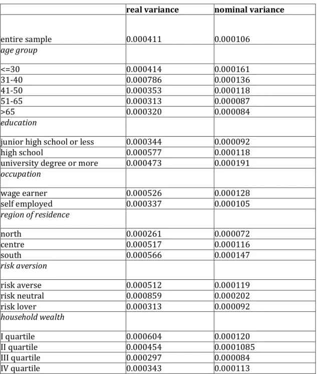
Table 1 presents the average values of the nominal and real measure of conditional variance of income growth. Average values are calculated by different groups: age, classes, occupation, education, area of residence, risk aversion and wealth quartiles. Looking at the table, we notice that households' reported uncertainty is higher for young people and wage earners. As expected, uncertainty perceived by risk averse households is higher than the one perceived by risk lovers. Moreover, those households who belong to the first and second wealth quartile report a higher measure of income growth variance than the relatively rich households.
Instead of relying on a particular utility function, I estimate a more general equation. Using this approach does not allow to estimate structural parameters. That means that, for example, the coefficient associated to the variance of income growth cannot be interpreted as the prudence coefficient, as this would mean assuming a CRRA utility, and having the variance of consumption growth instead of the subjective measure. However, estimating a more general equation allows me to exploit the unique measures of subjective expectation and variance of future income rate of growth, which could not be used assuming a specific form for households’ preferences.
Following Jappelli-Pistaferri (2000) the following equation is therefore estimated12:
(6) ΔlnCi,t1 α1agei,t1α2ΔlnFSi,t1 η(varredr)i,z,t β(eredr)θjµt1 vi,t1
where ΔlnCi,t1 represents the rate of growth of nondurable consumption, FSi,t1 is the change
12Actually, Jappelli and Pistaferri (2000) estimate a slightly different equation. They estimate the equation using eredn as an instrument for the effective rate of growth of income. Moreover, they introduce in the estimation a dummy which indicates whether the spouse of the household head has started working between t and t+1, in order to control for labour supply which might lead to biased estimates of predicted income growth, leading to spurious evidence in favour of excess sensitivity. However, I do not introduce labour supply indicators in my estimation. My aim is indeed to focus on the coefficient associated to the variance of income growth, looking at the strength of precautionary motive for saving, instead of testing for excess sensitivity. Actually, even following Jappelli and Pistaferri the results of the IV estimation do not affect the significance of the coefficient associated to the measure of uncertainty.
13
in family size, varredn is the subjective variance of nominal income growth and eredn represents the subjective expectation of income growth.
Actually, using the first and second moment of the subjective measure of income growth does not imply estimating a proper Euler equation, and therefore structural parameters estimation. An alternative way to estimate the effect of income uncertainty on households choices would be relying on direct empirical measurement of the relationship between uncertainty and wealth. However, empirical estimates are characterized by huge variations, which cannot be totally imputed to differences in the data used in the estimation. Furthermore, negative past shocks may affect households wealth holdings, resulting in a null wealth held for precautionary reasons. From this perspective, households might not exhibit an higher wealth accumulation, even though they may reduce current consumption.
The forecast error is made of two terms. The first term, θjµt1 represents an aggregate
component. In particular, θ captures the effect of unevenly distributed aggregate shocks j µt1
on the forecast error in consumption. The second term vi,t1 is a household-specific idiosyncratic component. The reason why the forecast error in consumption has such a specification is mainly to avoid excess sensitivity that may arise from the misspecification of the stochastic structure of the forecast error13. In order to cope with this problem, time dummies and
interaction between time dummies are included in the Euler equation.
Table 2 shows the estimation results of equation (6). Specification (1) excludes risk aversion. The coefficient associated to the conditional variance of the nominal income rate of growth is significant at 1% level. A positive and significant coefficient of the variance provides therefore evidence in favour of the precautionary saving hypothesis, as economic agents postpone consumption to the future by reducing current consumption.
In specification (2)-(4), in order to correct for the downward bias of the coefficient associated to the variance of the income rate of growth, I select the subsample of households interviewed in the periods 1989- 1991 and 1995 . Particularly, specification (2) includes the interaction term between household net wealth and absolute risk aversion. In specification (3) I only include households who report being risk averse14, but I do not incorporate the measure of risk aversion,
which is included instead in specification (4). Results show that including risk aversion leads to a better (and higher in magnitude) estimation of the coefficient associated to the precautionary motive. Intuitively, risk aversion is a key determinant of the precautionary motive for saving, since only risk averse households would be induced to save in order to face unexpected contingencies. Furthermore, the significance of the risk aversion coefficient implies that risk attitudes are an important determinant of households' consumption choices. From this perspective, accounting for attitudes towards risk in a regression solves an omitted variable problem. In line with Carroll and Kimball (2006) , the coefficient associated to the conditional
13If T , the forecast error goes to 0. However, in panels with small T and big N there is no guarantee that the forecast error goes to 0 as N.
14Risk averse households are those who report they would pay less than 10 million lire to buy the hypothetical security. Actually, they are the majority (1640 observations, 95.32% out of total sample).
14
variance of nominal income rate of growth is higher and better estimated.
4 Switching regression estimation.
So far, I have provided an empirical assessment of the relevance of households' precautionary motive for saving, suggesting a procedure to correct for the downward bias in the coefficient associated to the subjective variance of income growth. The next step would be to assess whether liquidity constraints significantly affect households reaction to labour income uncertainty.
From now on, cross sectional estimation will be performed, without exploiting the panel dimension of the data. Actually, because of a relatively low number of observations in the subsample of constrained households, a panel estimation is not feasible. Moreover, pooled estimation is also preferred because there is not enough variability in the probability of being constrained. Therefore, I carry out a cross sectional estimation, selecting only those households who were interviewed for 2 years, in order to avoid problems related to intra-household correlation. Moreover, instead of using the nominal measures of expected value and variance of income growth, I use real ones. This helps to avoid having the magnitude of coefficient associated to dependent variables in the regression determined by movement in nominal variables.
Table 3.1 presents results of the cross sectional estimation. In specification (2), the interaction term between household's coefficient of risk aversion and net wealth is included. We can notice that not only the coefficient associated to varredr is higher , but the risk aversion term is significant (at 10% level). Specification (3) includes the change in household income, whereas in specification (4) the latter variable is instrumented with the first moment of subjective income growth. Actually, varredr is always significant at 1% level.
The first step to investigate whether reaction to labour income uncertainty differs among constrained and unconstrained households is to perform a sample split. Earlier studies aiming to detect the relevance of liquidity constraints indeed rely on sample split techniques (Hayashi, 1985; Zeldes, 1989; Shea, 1995).
Table 3.2 presents sample split results, using several indicators of liquidity constraints15. In
specification (1) lb1 is used as a criteria to split the sample. lb1 takes value 1 if the household request for a loan has been rejected, or if the household did not ask for a loan fearing rejection ("discouraged" households). This is the survey-based measure of liquidity constraints provided by the SHIW. According to that, less than 4% of all population is considered constrained. An objection to this indicator of liquidity constraints regard the fact that the question about being turned down for a loan may pertain mainly to households who want to purchase a durable good (such as a house or a car), whereas the Euler equation refers to nondurable consumption. However, as pointed out by Jappelli et al. (1998), banks use to look at households' ownership of such goods in order to decide whether rejecting or not the loan. Consequently, using such an indicator would give a good idea of who is going to be constrained. The coefficient associated to
15See the appendix as far as frequency of households which can be considered as constrained/unconstrained according to several classification criteria.
15
varredr is higher for constrained rather than unconstrained households. This result also holds when the (effective) change in income is included in the estimation, and when the latter is instrumented with eredr (specification 2 and 3, respectively)
In specification (4) and (5), alternative definitions of liquidity constraints are used. This allows me to check for the robustness of my results and to increase the number of observations in each subsample. According to the second definition (lb2), households are constrained if their wealth is lower than 2 months’ income (Hayashi, 1984). The third definition (lb3) uses the level of indebtness (at time t) of the household in order to distinguish between constrained and unconstrained households. According to the third definition, a household is constrained if it has a ratio of financial liabilities/(real+financial asset) higher than 0.5.
Even using alternative definitions of liquidity constraints, the coefficient associated to the uncertainty indicator is still significant and higher for constrained rather than unconstrained households (table 4.2). In this perspective, adding a liquidity constraint (at time t) strengthen households' reaction to uncertainty. However, if a significant correlation exists between the selection equation's and the Euler equation's error term, sample split may lead to spurious estimation. Actually, the existence of such a correlation should be proved.
In order to correctly estimate the strength of the precautionary motive for saving across constrained and unconstrained agents, I will therefore rely on a switching regression approach. This approach has been used, among others, by Jappelli et al. (2001) and Garcia et al (1997). They look for the presence of liquidity constraints, looking at the significance and the magnitude of the coefficient associated with lagged income among constrained and unconstrained households. Here, I extend previous investigations on consumption behaviour by investigating the strength of precautionary savings among constrained and unconstrained agents. Therefore, I will focus on the magnitude and significance of the coefficient associated to the subjective variance of income growth, which is a measure of the precautionary motive for savings, among two different regimes. In this respect, my analysis is similar to Lee and Sawada (2009) who investigate the relationship between precautionary savings and liquidity constraints using survey data from Pakistan. However, my analysis differs from Lee and Sawada (2009) in three aspects. First of all, I use the unique piece of information regarding subjective expectations of income growth provided by the SHIW. Moreover, unlikely Lee and Sawada (2009) I take into consideration expected rather than effective liquidity constraints. As Carroll and Kimball (2001) and Jappelli and Pistaferri (2001) point out, excess sensitivity tests are not able to capture the effect of expected liquidity constraints. From this perspective, the coefficient associated to expected income growth may be not significantly different from zero - thus not rejecting the orthogonality condition provided by the LCPIH- if households expect to be constrained in the future. I will therefore extend Lee-Sawada analysis by estimating households' expectations of future liquidity constraints with a two-step procedure.
As far as the empirical estimation is concerned, I will rely on a switching regression framework in order to differentiate consumption behaviour among constrained and unconstrained agents. First of all, I estimate the Euler equation using an endogenous switching regression model with known sample separation rule using the survey-based indicator of liquidity constraints provided by the data. Then, I split the sample according to different cut-off values of households' estimated probability of being constrained.
16
In what follows, I present the general switching regression framework used to estimate the model with effective constraints as well as the model with expected ones.
The equation to be estimated on the whole sample can be rewritten as: (7) ΔlnCi,t1 α1Di,t1α2(varredr)i,z,t α3(eredr)i,t θjµt1νi,t1
where eredr and varredr are respectively, the expected value and the variance of real income growth at time t, Di,t1 includes demographic controls, such as age, sex, occupation, change in
family size and in the number of income recipients, and θ captures the effect of unevenly j distributed shocks. In the general specification of CRRA utility function with uncertainty and borrowing constraint, the lagged value of disposable income is included in order to take into account the shadow value of liquidity constraint. Here, following Jappelli and Pistaferri (2000) I include instead the expected value of income growth, in order to test for excess sensitivity of consumption to expected income changes. This way, I can look at the significance of the precautionary motive for saving, checking at the same time whether excess sensitivity is found among constrained agents. This is particularly relevant for my analysis: excess sensitivity tests are not indeed particularly powerful to test the presence of liquidity constraints. One of the reason is that excess sensitivity may be due to other reasons, different to borrowing constraints (myopia for example). Moreover, the Euler equation does not allow us to take into consideration future or expected liquidity constraints. However, the mere analysis of current constraints might be restrictive, especially in a country like Italy, where credit market imperfections discourage household to ask for a loan in the credit market. In my analysis I will therefore check whether excess sensitivity to expected income growth is found in the constrained subsample, looking at the same time at the significance of the second moment of income growth.
Considering 2 different groups of households (constrained and unconstrained), the previous equation can be written as a switching regression model with known sample separation rule, in the following way (see Maddala, 1986):
C t i, t C j t i, C t z, i, C t i, C C t i, α D α ( redr) α (eredr) θ µ ν C Δln 1 1 1 2 var 3 1 1 (8) (constrained regime) U 1 t i, 1 3 2 1 1 1 var ln (9)Δ C α D α ( redr) α (eredr) θ µt ν U j t i, U t z, i, U t i, U U t i, (unconstrained regime) (10) Xi,t γZi,t ui,t (selection equation) where: (11) C t i, t i, Δ C C Δln 1 ln 1 if I 1 (12) U t i, t i, Δ C C Δln 1 ln 1 if I 0
17
where I is a dummy variable which classifies households among constrained and unconstrained.
Specifically:
(13) I 1 if Xi,t 0 (14) I 0 if Xi,t 0
As Lee and Sawada (2009) point out, X can be rewritten as: i,t (15) Xi,t Ci,t Ci,t where t i,
C is the optimal level of consumption in absence of constraints, and Ci,t the effective
consumption when constraints are present. Jappelli (1990) and Hayashi (1985) approximate this difference as a quadratic function of observable cross sectional variables, such as current income, wealth and demographics. Assuming that the credit ceiling is a function of the same variables, we can write Xi,t γZi,t ui,t , that is the selection equation.
In the selection equation, Z includes indeed several variables predicting liquidity constraints. i,t
Earlier approaches, only included in Z financial variables. Zeldes (1989), for example, use a simple asset/income ratio in order to determine who is liquidity constrained. However, as Jappelli et al. (2001) point out, this approach might lead to misclassifications. Following Jappelli (1990) and Garcia et al. (1997) I assume endogenous liquidity constraints. That means allowing credit availability to depend not only on economic variables, but also on socioeconomic indicators.
The model described above is an endogenous switching regression model with known sample separation rule. Assuming endogenous switching means allowing a significant correlation between the error term of the main equation and in the selection equation, that is:
(16) σvu 0
The simplest case where the previous assumption is satisfied is when the regressors of equation (8) and (9) are included in the selection equation (10). However, this is only one of the cases of endogenous switching16. Actually, the existence of a significant correlation between the error
term of the main equation and the error term of the selection equation needs to be proved empirically. Some authors as. Garcia et al. (1997) argue that assuming endogenous liquidity constraints is not plausible, since households do not choose to be constrained. From this perspective, households request for a loan can be viewed more as the outcome of credit
16From this perspective, the inclusion of subjective moments of income growth as explanatory variables of the probability of being constrained can be explained by taking into consideration the fact that the measure of constraints we are using encompasses both demand and supply-side factors. From this perspective, subjective average and variability of future income growth - albeit not affecting the probability the loan is rejected- are likely to affect household probability of asking for a loan. This is true, in particular, when expected constraints are taken into account.
18
related factors rather than household decisions. However, as pointed out by Lee and Sawada (2009), the household can choose to be unconstrained, (i.e. having a desired level of consumption lower than the effective one). Having defined the liquidity constraint indicator as dependent on the gap between desired and effective level of consumption, assuming exogeneity of liquidity constraint is not so straightforward.
I estimate the model through a full information maximum likelihood (FIML) estimation17. This
allows to simultaneously estimate the binary and continuous part of the model, and to avoid inconsistent estimates of standard errors18. Actually, if σ 0
vu , estimating separately equation
(8) and (9) would lead to spurious results.
Obviously, the correlation between the error term in the main and in the selection equation needs to be proved. If the correlation term is found not to be statistically different from 0, the equations describing each regime and the sorting equation are independent, so that an exogenous instead of endogenous switching model should be estimated.
Actually, if the correlation term between the error term in the main and in the selection equation turns out to be zero, the model reduces to OLS.
The switching regression model above can be rewritten in one equation as: (17) ΔlnCi,t1 θ2Wi,t1(θ1θ2)Wi,t1Ii,t εi,t1 where: (18) U 1 t i, 1 3 2 1 1 1
1W α D α (varredr) α (eredr) θ µ ν
θ t U j t i, U t z, i, U t i, U t i, and (19) C t i, t C j t i, C t z, i, C t i, C t i, α D α ( redr) α (eredr) θ µ ν W θ2 1 1 1 2 var 3 1 1
I is the indicator of borrowing constraints. So if I 1 : (20) ΔlnCi,t1 θ1Wi,t1 εi,t1
whereas if I : 0
(21) ΔlnCi,t1 θ2Wi,t1εi,t1
Tables 3.3 (a) and (b) presents the results of the estimation of the endogenous switching
17Actually, this method gives more efficient estimates rather than heckman two-step approach.
18Lee and Sawada estimate instead a V type tobit using treatment effect model instead, which is a particular case of the switching regression approach. Particularly, treatment effect models does not allow the effect of the treatment to vary across regimes.
19
regression model. In the selection equation the probability of being constrained depends on age, education, wealth, wealth squared and geographical area. Moreover, in order to improve upon the identification of the selection equation I add as a regressor the interaction term between the percentage of bank counters in each region and the average number of inhabitant in the city where the household lives19. Intuitively, this variable should be strongly correlated with the
probability of being liquidity constrained but not correlated with changes in consumption growth. Actually, we should observe, ceteris paribus, that the higher the number of bank branches in a certain town, the higher the opportunity to ask for a loan in the credit market and, therefore, the probability of being constrained.
In specification (I) I use a survey based indicator of borrowing constraints (lb1). More specifically, the dummy variable lb1 takes value 1 if the household at time t has asked for credit and the loan has been rejected or if the household did not ask for credit fearing its request may be rejected ("discouraged borrowers").
In specification (1), the coefficient associated to the variance of real income growth for constrained households is positive and significant at 5% level, whereas it is lower for unconstrained ones. These results are in line with Carroll (2001). Actually, a complementarity relation exists between precautionary savings and liquidity constraints, so that the introduction of a liquidity constraint increases the precautionary motive. Rho0 and Rho1 represent the correlation term between the error term of the selection equation (10) and error terms of equations (8) and (9), respectively.
Rho1 is highly significant in all the specifications, for both constrained and unconstrained households. That suggests that the correlation between the error term in the main equation and in the selection equation is nonzero, and the use of an endogenous switching is justified. Moreover, Rho0 and Rho1 have the "right" sign in both subsamples. For constrained households, Rho1 is positive. It means that a constrained household has higher consumption growth than a random household. In the subsample of unconstrained households instead, Rho0 is negative, meaning that unconstrained households have lower consumption growth than a random household.
Actually, no excess sensitivity is found either for constrained or for unconstrained households. The same result has been found by Jappelli and Pistaferri (2000) in the entire sample and dividing the subsample according to the wealth/income ratio. Actually, this result does not invalidate my analysis and it can be explained taking into account the peculiarity of Italian credit markets. Due to high downpayment requirements and high transaction costs, Italian household do not trust credit markets. As Guiso and Jappelli (1994) point out, Italian households who do not obtain a loan in the credit market might ask for help to parents or friends in order to overcome credit market deficiencies. As a consequence, even if they are constrained in the credit market, households do not show excess sensitivity to expected income growth, since they can ask "informal" networks (relatives, friends, etc.) for funds.
Moreover, the same lack of confidence in credit market may lead Italian household to save more over time, in order to have some kind of protection against future income shocks. In this perspective, a classical test of excess sensitivity has a relatively weak power, since households
20
may save more over time in order to protect against their restricted access to liquidity.
Finding an high precautionary motive but no evidence for excess sensitivity gives therefore further strength to the complementarity relation between precautionary savings and liquidity constraints. Households do not show excess sensitivity because they strongly save "precautionally' in order to face future risk, including the impossibility to get additional funds from a bank or a financial institution.
In order to check robustness of the results, in specifications (2) and (3) the switching regression is implemented using alternative indicators of liquidity constraints. In specification (2) the survey based indicator of liquidity constraint lb1 is combined with lb2 , whereas in specification (2) lb2 is combined with lb3. In this sense, a household is defined as presumably constrained if at least one of the dummies (lb1 or lb2, in specification (2) or lb2 and lb3 in specification (3)) is equal to one. On the contrary, the household is defined as presumably unconstrained if all these dummies are jointly equal to zero.
Actually, even when alternative definitions of constraints are considered, the coefficient associated to varredr is higher for constrained rather than unconstrained households. However, Rho1 and Rho0 are no longer significant. This is in line with the strand of literature which criticize the use of asset-based indicators in order to identify who is constrained in the credit market. From this perspective, a direct survey-based indicator of borrowing constraints provides a more precise criteria to identify those obstacles in credit markets which affect households saving and consumption decisions.
5. Switching regression estimation with perceived probability of being constrained.
As Carroll and Kimball (2001) point out, expected liquidity constraints might affect households' consumption choices as well as effective ones. In particular, they argue that precautionary saving may arise from the possibility that constraints may bind in the future, even if a household is not effectively constrained at the time of consumption and saving choices. They formally show indeed that once the concavity of consumption function is induced, by liquidity constraints or by uncertainty, it propagates backwards. In this perspective, households who expect liquidity constraints to bind in the future may save more, in order to make the constraint less likely to bind.
Here, I try to capture the effect of households' expectations about future constraints on their consumption and saving choices. In order to estimate households' expected probability of liquidity constraints, I rely on a two-step procedure. I first estimate household probability of being constrained at time t, as a function of demographics, current wealth and current income. Formally:
(22) Prob(liq.constraint)t β(Xt)εt
where Xt includes demographics and financial variables at time t, and ε is the error term. The t
21
being constrained in the future:
(23) Pr int 1 t t1 t1
^ t
t[ ob(liq.constra ) ] βE(X ) ε
E
where Xt1 includes future variables known at time t. In particular, the expectation at time t of
income at t is calculated multiplying current labour income for the subjective expectation of 1 income growth. In the same way, future (expected) wealth is obtained from current net wealth, using subjective expectations about future inflation. In this perspective, income and inflation subjective expectations provide a useful tool, letting us be able to know to what extend expectations about future variables affect households' perception about future constraints.
Estimated probabilities are then used to distinguish among constrained and unconstrained households. In particular, an household is classified as constrained if the estimated probability is higher than a certain cut-off value20.
Table 4.1 presents results of a sample split using different cut-off values of the probability estimated in the previous section. In particular, in specification (1) an household is defined as constrained when the expected probability of future liquidity constraints is higher than 10%; in specification (2) instead, the cut-off value is 20%21. Even in this case, the coefficient associated to
the variance of subjective income growth is higher for constrained rather than unconstrained households22.
One issue with the credit constraint indicator is indeed that this is the probability that the household is turned down. This is equal to the probability of applying for the loan times the probability of being turned down conditional on applying. The first reflects demand, whereas the second reflects supply for credit.
Previously I have defined a household as liquidity constrained if the desired level of consumption is higher than the effective one. In this perspective, a household can be considered not constrained in two cases. First of all, if it is able to obtain all the needed resources. Secondly, it might be that the household is a saver; in this case it would use the resources the household piled up in the past rather than asking for a loan. Whereas the first case is related to supply-side factors-i.e. a well developed loan market- the second one reflects households' specific attitudes towards saving and consumption. As far as our analysis is concerned, the first case is more relevant than the second one, since we are arguing that households’ reaction to labour income uncertainty is strongly affected by credit market imperfections (therefore, credit supply related factors).
20Note that the dependent variable in the probit regression is a dummy which takes value 1 if liquidity constraint indicators lb2 or lb3 take value 1, 0 otherwise. We tried alternative specifications using lb2 or lb3 alone, or lb1. Actually, results remain basically unaffected.
21As shown in the appendix, the average value of the estimated probability is around 13%.
22A switching regression has also been performed. Actually, empirical results are basically the same, albeit correlation coefficient rho1 and rho2 are not significant. Results are not reported but they are available upon request.