A Markov chain model for dependability evaluation and fault prediction on UPS systems

(1)

POLITECNICO DI MILANO

Master of Science in Computer Science and Engineering Dipartimento di Elettronica, Informazione e Bioingegneria

A Markov chain model for

dependability evaluation and fault

prediction on UPS systems

Supervisor: Prof. Francesco Amigoni

Co-supervisor: Prof. Letizia Tanca

M.Sc. Thesis by:

Antonio Gianola, 877235

(2)

(3)

(4)

(5)

Abstract

Nowadays, electricity is one of the key assets in most of the activities. Just think of the importance of this power to companies, hospitals, or data ware-houses where a blackout of a few minutes could cause injuries, businesses disruptions, or data loss. One of the solutions most used by companies to deal with outages involves the use of Uninterruptible Power Supply (UPS), electrical systems able to provide energy to a load when the input source fails. It is redundant to specify how essential these devices are and how much dependability is crucial to the system. Up to now, this last property is mainly guaranteed by specific and sophisticated design techniques, and by log files generated automatically to keep track of how the system behaves. Usually, the files are manually managed by the maintenance service, that has the purpose of locating and replacing the damaged components. Since this approach is mostly manual and has several limitations in terms of prediction capabilities, the need came to derive automatic techniques for analysing the generated data and creating estimates on how the system will behave in the future. Without any knowledge of the domain and of the system, by using Artificial Intelligence techniques. In this thesis we build a model that tries to capture the events leading to the failures and to predict the happening of malfunctions, allowing an operator to repair the system before it fails. We focus our attention on Markov chain models, and through the thesis, we discuss the operations performed to build the models in our application. In the end, we develop an easy-to-use software program able to compute and display the models.

(6)

(7)

Sommario

L’energia elettrica è una delle risorse chiave per la maggior parte delle at-tività. Basta pensare alla sua importanza per le aziende, gli ospedali o i data warehouse dove un blackout di qualche minuto può causare infortuni, danni economici o perdita di dati. Una delle soluzioni più usate per contrastare le interruzioni di energia elettrica consiste nell’utilizzo dei gruppi di conti-nuità (UPS), sistemi elettrici capaci di fornire elettricità al carico quando la sorgente non funziona. È superfluo specificare come questi dispositivi siano essenziali e come l’affidabilità sia un aspetto fondamentale di questi sistemi. Ad oggi quest’ultima proprietà è garantita da specifiche e sofisticate tecniche di progettazione e da file di registro generati automaticamente per tenere traccia del comportamento del sistema. I file solitamente vengono controllati manualmente dal servizio di manutenzione che ha il compito di sostituire eventuali componenti danneggiati. Dato che queste tecniche manuali hanno diverse limitazioni in termini di previsione dei malfunzionamenti futuri, è sorto il bisogno di creare un metodo automatico capace di analizzare i dati generati e fornire stime di come il sistema si comporterà in futuro. Senza nessuna conoscenza di dominio ed utilizzando tecniche di Intelligenza Artifi-ciale, in questa tesi costruiremo un modello del sistema capace di catturare le dipendenze fra i guasti e prevedere l’arrivo di malfunzionamenti, perme-ttendo quindi ad un operatore di riparare il sistema prima che si guasti. Concentreremo la nostra attenzione sulle catene di Markov e, durante la tesi, descriveremo le operazioni compiute per creare il modello nel caso della nos-tra applicazione a sistemi UPS. Infine, svilupperemo un programma software capace di generare e visualizzare i modelli.

(8)

(9)

List of Figures

2.1 An example of Markov chain with three states, taken from [1]. 13 2.2 The figure shows the parameters of an HMM. Xi is a state, yi

is a possible observation, aij is the transition probability, and

bij is the observation probability [2]. . . 16

3.1 The figure shows how the ∆T works in the event log file. . . . 27 3.2 The figure shows how the chain length parameter (N ) works

when a sequence is too long. . . 28 3.3 The figure shows how the associations between alarms a1, a2

and maintenance actions f1, f2, f3 look like. . . 29

3.4 By using the graph representation, the figure shows an exam-ple of a chain. . . 29 3.5 By using the graph representation, the figure shows an

exam-ple of three chains whose have shared states. . . 30 4.1 This figure shows the number of times in which every alarm

appears in the event log file. . . 37 4.2 This figure shows the number of times in which every message

appears in the event log file. . . 37 4.3 The figure shows a simple graph representing the correlations

between the events 8205, 9202, and 9203. . . 38 4.4 The figure shows the correlation between an alarm (4105) and

the messages immediately before (8405,4102). . . 39 4.5 The figure shows the relations between a set of messages (8405,4102)

that are associated with the same alarm (4105). . . 40 5.1 The figure shows the writing sequence done by the event logger

(14)

5.2 The figure shows the event with code 1203 represented by the

code state representation. . . 53

5.3 The figure shows the graph produced by considering the chains in Equation 5.13. . . 54

5.4 This figure shows the event 1203 coming from the devices with id 1 and 2 appears in the id/code representation. . . 55

5.5 This figure shows a graph representing the chains of Equation 5.14. . . 56

5.6 This figure shows the resulting graph obtained by considering the chains defined in Equation 5.15. . . 57

5.7 This figure shows two states represented by using the Level**id/code representation. 1 ∗ ∗2/1203 means that the message with code 1203 from Device 2 is in the first position of its chain. . . 58

5.8 The figure shows the pairs reported in Equation 5.18 organized in a graph. . . 60

5.9 The figure shows the model without considering any postpro-cessing. . . 65

5.10 The figure shows the associations between alarm 8521 and its maintenance actions. . . 66

6.1 The figure shows how the main components of the application exchange messages. . . 70

6.2 The figure shows the first window of the application. . . 72

6.3 The figure shows the class diagram of the view. . . 72

6.4 The figure shows a portion of a real transition matrix. . . 74

6.5 The figure shows a portion of the model reported in Figure A.1 of Appendix A. . . 76

6.8 The figure shows a portion of the model reported in the Figure A.2 of the Appendix A. . . 79

(15)

6.11 The figure shows a portion of the model reported in Figure

A.5 of Appendix A. . . 82

6.14 The figure shows a portion of the model reported in Figure A.8 of Appendix A. . . 85 A.1 Model 1. . . 98 A.2 Model 2. . . 100 A.3 Model 3. . . 102 A.4 Model 4. . . 103 A.5 Model 5. . . 104 A.6 Model 6. . . 105 A.7 Model 7. . . 107 A.8 Model 8. . . 109

(16)

(17)

List of Tables

2.1 This table shows the typical Markov models used depending on the situation [3]. . . 9 3.1 This table shows how the event log file is structured. . . 23 3.2 This table shows how an UPS reports an event. . . 24 3.3 This table shows the information contained the UPScale. . . . 24 4.1 This table shows the information extracted from the event log

file of Table 3.2. . . 34 4.2 This table shows the relation between event code and event

type. . . 35 4.3 This table shows the relation between event code and

mainte-nance actions. . . 35 4.4 This table shows the number of events for each device. . . 36 4.5 This table shows the number of events by type for each device. 36 4.6 This table shows the number of events by type for each day. . 36 4.7 This table shows the mean, the standard deviation, the

mini-mum, and the maximum of the TBE for each day. . . 41 4.8 This table shows the mean, the standard deviation, the

mini-mum and the maximini-mum of the TBE for each device, for each day. . . 42 5.1 This table shows a portion of the dataset used to build the

chains. . . 47 5.2 This table shows a portion of the dataset including the

times-tamp. . . 49 5.3 This table shows a portion of the dataset where we have many

(18)

5.4 This table shows a portion of an event log file where three messages are registered at the same time. . . 51 5.5 This table shows a portion of an event log file where one

mes-sage and one alarm are coming at the same time. . . 52 5.6 This table shows a portion of the dataset including the

times-tamp, the device id, and the event code. . . 53 5.7 This table shows a portion of the dataset with 6 messages and

2 alarms. . . 57 5.8 This table shows the branching factor of the model with

re-spect to the state representation. . . 61 5.9 This table shows the number of the states with respect to

different states representation and model parameters. . . 62 5.10 The table shows a row of the transition matrix. . . 63 5.11 This table shows the relation between event code and

mainte-nance actions. . . 65 5.12 This table shows two records of the service log file. . . 66 6.1 This table contains a summary of the primary methods of the

(19)

Chapter 1 Introduction

Our world is more and more dependent on electricity: anyone who offers us a service or produces goods needs it. Just think of the importance of this power to companies, hospitals, or data centers, where a blackout of a few minutes could cause injuries or fatalities to people, severe businesses disruptions, or data loss.

For these reasons, companies have implemented several solutions to guar-antee theirs services in face of electric power shortages. One of the most used solutions involves Uninterruptible Power Supply (UPS), electrical sys-tems able to provide energy to a load when the input source fails. These systems can increase their size easily from units designed to protect a single computer to large units powering data centers. The largest UPS is a 46-Megawatt Battery Electric Storage System, in Fairbanks, Alaska, built by ABB in 2003, and it provides power to the city during outages [4].

It is redundant to specify how these devices are essential and how the dependability is a crucial aspect for them. Up to now, this property is guar-anteed by specific and sophisticated design techniques and by log files gen-erated automatically to keep track of how the system behaves in order to repair it as soon as possible in case of failure. There are several limitations of this approach solutions; the design phase can be performed only by skilful people, without any chance to take into account the actual behaviour of the system during its operation and therefore without considering the hidden variables that affect the rising of failures. By using the log files, we must necessarily wait for a failure of the system before performing any reparation. Moreover, a manual analysis of these files could require a long time affecting the repairing time. Therefore, the need to create an automatic method able

(20)

to analyse the data and provide insightful information on the working of the system.

In this thesis, we focus our attention on the log files provided by a com-pany and produced by a complex system composed of different UPSs, with the goal of creating a behavioural model able to relate with each other the events occurring within the devices. Our objective is to generate a series of models based on Artificial Intelligence techniques, to predict the happening of malfunctions, and allow operators to preventively act on the system be-fore it fails. In particular, we will focus on Markov chain models, statistical models capable of capturing dependencies between events occurring during time. In the thesis, we will not use any knowledge of the system, therefore all the dependencies will be extracted automatically from the data.

During the thesis, we encounter the restriction of having a limited amount of data; an initial analysis is devoted to understand how these data are generated from the UPS system and written on the log file. This problem will, in fact, limit the prediction capability of the created models.

We will associate to each other the events of a UPS system by developing a method able to extract the dependencies between them. Our goal is to create a model that includes the relations between the events occurred in a system. For each association between events, we will include some attributes able to quantify their strength. We will especially pay attention to the post-processing phase, fundamental in our context to add the maintenance actions needed to repair a UPS in case of failure and to display the transitions with graphical techniques. In the end, we will create a software program able to ask the user for the parameters and to generate a model reported as a graph in order to improve the immediacy and clarity of fruition by an operator of the company that provided the data. Through this thesis, we will demon-strate the utilisation and the effectiveness of our approach in dependability evaluation and fault prediction for UPS systems.

The literature offers interesting papers related to our work, spanning from the use of Bayesian network for dependability analysis on circuit breaker [5] to the use of a Markov chain to model the correlations between faults in a complex system [6]. Different papers use predictions techniques based on domain knowledge to elaborate a model of a UPS system [7–9]. However dif-ferently from these works, we do not have any prior knowledge of the system, but our analysis is based only on the events produced and the associations among them.

(21)

The thesis is structured as follows:

• Chapter 2 (Preliminary notation and state of the art): in this chapter we present the state of the art and the notation used to define the Markov chain and Hidden Markov model.

• Chapter 3 (Problem setting): in this chapter we define the context of the thesis, its main goals, the data provided, and the tools used. • Chapter 4 (Preprocessing and data analysis): here we show the

process followed to analyse the data provided by the company.

• Chapter 5 (Markov chain model): in this chapter we present the steps required to build a Markov chain, including we also include the postprocessing phase.

• Chapter 6 (Implementation details and examples of use): we describe the architecture developed and we compare how the model behaves by changing its parameters.

• Chapter 7 (Conclusions and future work): we briefly summarize the thesis and discuss the future steps to improve our work.

(22)

(23)

Chapter 2 Preliminary notations and state

of the art

In this chapter, we review the state of the art of the most important tech-niques relevant to this thesis. In Section 2.1, we show the different approaches to analyse the System Dependability by comparing the Measurement-Based methods and the Model-Based methods. In Section 2.2, we discuss the dif-ferent types of Model-Based methods by comparing the Combinational ap-proach and the State-Space apap-proach. In Section 2.3, we present the Markov models by focusing our attention on Markov Chain and Hidden Markov Mod-els. In Section 2.4, we review the most important work related to my thesis.

2.1 System dependability

For many physical systems, one of the most important properties is the de-pendability. The dependability of a system is its ability to deliver a service that can be trusted. A service is defined as the set of outputs perceived by the user and a system failure is a deviation from the correct service and it is usually assumed that failures are caused by random events. The most critical dependability attributes are reliability, availability, safety and maintainabil-ity.

A system does not always fail in the same way, according to [10] there are three main classes of faults: design faults, physical faults and interaction faults. When a design faults, most of the time, it is generated due to designers or developers who can forget unforeseen situations of the system. A physical

(24)

faults depends on the components used to build the system. The typical way to remove these faults consists of replacing the component with a new one. An interaction faults regards the exchange of messages among the system components. Most of these faults can be avoided by providing a deepened analysis during the design phase.

Some important tools which designers and developers of a dependable system must count on, according to [10], are: fault prevention, fault toler-ance, fault removal and fault forecasting: these aspects must be considered to improve the dependability of a system. For instance, the fault removal concerns how to reduce the number or severity of faults and is related to monitoring and maintenance strategies. In order to minimise the mainte-nance cost, two policies are possible: proactive maintemainte-nance tries to prevent the component or system failure. While in the reactive maintenance the failure of the system triggers an action. The fault tolerance is the property of delivering the correct service in the presence of faults and it is typically reached by duplicating some components in the system, according to [11], the redundancy can be performed on different levels: hardware, software, time or information, depending on the system a specific level may be better than another. Fault prevention and forecasting are archived by using fault identification and detections strategies.

According to [12], there are two main methods to evaluate and analyse the dependability of a system:

• The Measurement-Based method requires to observe and to measure the behaviour of the components of a system in its operational envi-ronment; This method gives the most credible results, but it may be unfeasible or too expensive. In some cases, a copy of the system is tested to measure these parameters and, it could cause the ending of the working life of the system with money wasting.

• The Model-Based method is preferable in those cases where is impossi-ble to replicate a copy of the original system. This method involves the construction of a model by defining and abstracting the main elements and properties of the system. The resulting model should be accurate enough to give a proper evaluation of the dependability.

(25)

2.2 Model-based methods

Dependability evaluation research comes up with a variety of Model-based methods. While each method relies on a specific level of abstraction and/or system characteristics, all the Model-based methods share some prior domain knowledge. We distinguish two different main paradigms of Model-Based methods: Combinational models and State-Space models.

Combinational models represent the system by using logical connections. These methods are also known as qualitative model-based representations [13]. In these models, the prior domain knowledge is composed of a funda-mental understanding of the process using experience and evidential informa-tion. The model is developed thanks to the understanding of the physics of the process with the aim to capture knowledge in a formal methodology. The structure of a system is expressed by using logical interconnections of compo-nents. The notation usually is quite intuitive and easy to manipulate. Many combinational model techniques have been applied to dependability evalua-tion and fault detecevalua-tion problems: Fault Trees, formally described by [14], Reliability Block Diagrams [15], and many other models.

Combinational model techniques have also been applied to UPS systems using the Fault Tree Analysis to identify all the potential causes leading the system failure [7]. That work proposes a technique to estimate the failure rates, the mean time between failures, and the reliability of five UPS topolo-gies. In that work, to develop the model it is required a previous knowledge of the system in terms of main sub-components and interconnections. Moreover, they don’t use any specific data to compute the overall failure probability but they consider the literature probability of an event causing a failure. Also the Reliability Block Diagram method to model UPS system availability and reliability is proposed [8, 9], however, this work does not consider the causes of a failure and it is difficult to perform a fault identification analysis.

Note that It is not always possible to use a combinational technique since sometimes there is not enough prior domain knowledge to model the sys-tem behaviour. Moreover, the modelling power if this technique might be inefficient because the combinational techniques assume the statistical inde-pendence of the events. In real systems the events are not independent, in these cases, a State-Space model is more advisable.

State-space models represent the behaviour of the system in terms of reachable states and probabilistic dependence between states. We assume

(26)

that there is a hidden state of the system that evolves with time, possibly as a function of the inputs, and generates the observations. The goal is to exploit the observation to infer the hidden state up to the current time. This category of models is also known as History-based methods [16]. State-Space models provide a general framework for analysing deterministic and stochas-tic dynamical systems that are measured or observed through a stochasstochas-tic process. The prior knowledge needed, in this case, is only composed of a large set of historical process data. This knowledge is transferred to the model after a feature extraction process that has the aim to extract all the useful information from the historical data. The state space analysis may be computationally expensive because of the number of states of the model and the number of features used to elaborate it. Models as Markov chains [17], and Petri nets [18], and Bayesian networks [19] belong to this category. In all these methods, a state can be considered as a specific configuration of the system that holds for an interval of time. An event can change the system configuration and consequently the state of the model. Given a set of ran-dom variables that represent the system configuration at a specific time, the modeller has two main choices: either specifying the joint probability distri-bution or asserting a suitable set of independence assumptions, that can be learned from data. If we define every variable as independent of the others, the joint distribution can be easily obtained by multiplying the probabilistic parameters. However, assuming the complete independence of the variables is unrealistic for most systems. By considering a complete dependence of the variables, we create an opposite problem, in which it is computationally impossible to analyse and create the state space. The best solution consists of providing a reasonable set of information concerning the dependence and independence of the variables.

There are many published papers about dependability and fault analysis by using State-Space models. For instance [20] has studied how to develop a Bayesian network to support the fault analysis and the reliability estima-tion of a power system nodes architecture. The result is a versatile tool to automate the construction of models driven by probabilistic distribution of variables. A use of State-Space model for failure analysis is presented in [18], where the authors try to overcome the Combinational models by developing a Petri network, that can be constructed to represent the cause-effect relation-ship between events. Fault detection and dependability analysis have also been applied to intermittent faults of electronic system [21], where the many

(27)

factors that may cause intermittent faults are modelled by using a Markov model. The data are taken from US military and electronic industries. The faults are divided into three categories: drift, intermittent, and burst fault and the goal of the model is to determine the true alarms and false alarms. The produced model is a three-state Markov model able to reduce the num-ber of false alarms and increase the fault detection rate with respect to the traditional two-state model.

The approaches to dependability evaluation and fault detection described in the literature cannot be applied to our problem. We must exclude Combi-national models because we have not enough domain knowledge to elaborate a model. Moreover, we cannot use directly the State-space modelling tech-niques because of the structure of the data, in which it is not clear which are the dependent variables and the independent variables. An interesting paper [5] proposes a Bayesian network framework for supporting the opera-tions of circuit breakers. The aim of that paper is to introduce the use of AI tools easy to be integrated and easy to use and the input data are taken from the literature and regard the reliability of circuit breakers. We can identify some analogies between that work and this thesis, especially in the goals of the models developed. In this thesis, we use Markov chains to create an in-novative model for operations and support in power-critical applications by modelling the event correlations.

2.3 Markov model

In probability theory, a Markov model is a stochastic model used to model randomly changing systems. There are four common Markov models that are used in different situations, depending on whether every state is observable or not, and on the presence of autonomous or controlled circumstances [3].

Fully Observable Partially Observable

Autonomous Markov chain Hidden Markov model

Controlled Markov Decision process Partially Observable Markov Decision process

Table 2.1: This table shows the typical Markov models used depending on the situation [3].

(28)

• Markov chain: it is the simplest Markov model. It represents the state of a system through continuous or discrete time. All the states of the model are fully observable by the observer. We describe the Markov chain in Section 2.3.1.

• Hidden Markov model: it is a Markov chain for which the states are partially observable. An observation is related to the state of the system, but it is typically insufficient to precisely determine the state [2]. We describe the Hidden Markov model in Section 2.3.2.

• Markov Decision process: it is a discrete time stochastic control process. It provides the mathematical framework to model decision making situations where the outcome is partially random and partially decided by an agent. At each time step, the decision maker may choose an action (a) based on the available set of actions (A) and the current state x. The model responds by randomly changing the state into s0 and giving reward R(s, s0) [22].

• Partially Observable Markov Decision process: it is a generali-sation of a Markov Decision process in which an agent cannot directly observe the system. An agent chooses the best action depending on the maximisation of the expected reward over a possible infinite hori-zon. [23]

In our problem, it is impossible to identify an agent that takes actions and affect the evolution of the system. So, we focus our analysis on Markov chain model and Hidden Markov model.

2.3.1 Markov chain model

A stochastic process is a family of random variables, namely {Xn} where

n = 1, 2, 3.... The value xn of the random variable Xn at the time n is called

the state of the random variable at that time instant. The set of all possible values that the random variable Xn can assume is called state space, namely

S.

When the dependence of xn+1 is entirely captured by the dependence on

the last sample xn we say that the stochastic process is a Markov chain.

More precisely, we have:

(29)

where : xn+1, xn, ..., x1 ∈ S

Which is called Markov Property. We provide a definition of this property. Definition 1 (Markov Property [24]:) A sequence of random variables X1, X2, ..., Xn, Xn+1 forms a Markov chain, if the probability that the system

is in state xn+1, given the sequence of past states it has gone through, is

exclusively determined by the state of the system at time n.

We can think of the Markov chain as a generative model, consisting of a number of states linked by transitions. Each time a state is visited, the model outputs the symbol associated with that state.

The process is also characterised by a transition probability defined over every combination of states. Let

P (Xn+1 = j|Xn = i) = pi,j (2.2)

denote the transition probability from the state i to the state j. If the transition probability between two states is fixed and does not change with time, the Markov chain is said to be homogeneous.

Definition 2 (Homogeneous Markov chain [17]) An homogeneous Markov chain on a finite or countable set S is a family of random variables X0, X1, ..., Xn

such that:

P (Xn+1 = j|Xn = i) = pi,j (2.3)

The distribution of the Markov chain is uniquely determined by the initial distribution and the transition probabilities

φ(i) = P (X0 = i) Initial distribution (2.4a)

Pi,j = P (Xt= j|Xt−1 = i) T ransition probability (2.4b)

Definition 3 (Initial distribution [17]) For each i ∈ S let φ(i) be the probability of the system to be in state i at time n = 0 where we assume that:

φ(i) ∈ [0, 1] (2.5a)

X

i∈S

(30)

In order to be valid, all the transition probabilities of a Markov chain must satisfy the following properties:

X

j∈S

pi,j = 1 ∀i ∈ S (2.6a)

pi,j ≥ 0 ∀i, j ∈ S (2.6b)

In case of a system with a finite number of states, the transition can be compactly represented by using the transition matrix P . The transition matrix of a system composed by K states is:

P =      p1,1 p1,2 . . . p1,K p2,1 p2,2 . . . p2,K .. . ... . .. ... pK,1 pK,2 . . . pK,K      (2.7)

A condition on P is that each row must add to unity.

The definition of transition probability given in Equation 2.3 may be generalised to cases where the transition from i to j take place in a fixed number of steps. Let m be the number of steps and denote pm_i,j the m-step transition probability.

P (Xm+n = j|Xn = i) = pmi,j (2.8)

pm

i,j may be seen as the sum over all intermediate states, k, through which

the system passes in its transition from i to j. pm+1i,j =

X

k

pmi,kpk,j (2.9a)

p1i,k = pi,k (2.9b)

A directed graph gives the dynamics of a Markov chain with a state space S and transition matrix P with nodes representing the individual states and the edge labelled by the probability of possible transition. In Figure 2.1, a simple example of a Markov chain is shown using a directed graph. According to the figure, a bull week is followed by another bull week the 90% of the time, a bear week 7.5% of the time and a stagnant week by another 2.5%. Labelling the state {1 − bull, 2 − bear, 3 − stagnant} the transition matrix is: P =   0.9 0.075 0.025 0.15 0.8 0.05 0.25 0.25 0.5   (2.10)

(31)

Figure 2.1: An example of Markov chain with three states, taken from [1].

Now, we consider the problem of determining the probability of a sequence of states. Given a sequence of states s0, s1, ..., sn ∈ S where n is the length

of the sequence, and pi,j the probability reach the state sj given the state si.

The probability of the entire sequence is computed as:

P (s0, s1, ..., sn ∈ S) = n

Y

i=1

pi-1,i (2.11)

This allows the model to be applied to sequences of arbitrary length. By considering the example introduced by the Figure 2.1, we can compute the probability of the sequence (Bull, Bull, Bear, Stagnant), respectively (s1, s1, s2, s3) by using 2.11.

P (s1, s1, s2, s3) = p1,1∗ p1,2∗ p2,3 (2.12a)

= 0.9 ∗ 0.9 ∗ 0.075 ∗ 0.05 = 0.003 (2.12b) The most known examples of Markov chains are:

• Random walk: it is a stochastic random process, that describes a path that consists of a succession of random steps on some space such as the integers. An elementary example can start from 0 and move +1 or -1 with equal probability. The move depends only on the current position because of the Markov property. The transition probability to reach the next smaller or larger integer are both 0.5.

(32)

• The weather example: given the weather at the present moment, a Markov chain can predict the weather in the next days. The evolution of the weather can be modelled as a stochastic process.

2.3.1.1 Learning

When the transition probabilities are unknown we can learn them automat-ically from the historical data of the system. The method implemented in this thesis tries to extract a set of pairs from a set of sequences of states. A pair represents a transition of the final model and it can be written as (si, sj). To find pi,j we have to count the number of times where from the

state i we observe a transition to j, and divide it from the total number of pairs that have i as starting point. Let us give a formal definition of the concepts explained above:

s0, s1, ..., sn ∈ S (2.13a)

Q = (q0, q1, q2, ..., qT) | qi ∈ S (2.13b)

Where S is the set of states and Q is the sequence of states observed in a single execution of the system. By observing the system K times, we can obtain a set of different sequences with different length T0, T1, ..., TK. All

these sequences are collected in D, the set of all the data we have. Qk = (qk0, q k 1, q k 2, ..., q k T k) (2.14a) D = {Q0, Q1, Q2, ..., QK} (2.14b)

The next step consists of exploding the sequences we have in a set of pairs. Every pair (si, sj) represents an association between si and sj coming from

the sequences we have. All the pairs generated are inserted in the set F . Ck = {(qkt, qkt+1)|∀t ∈ 0 : Tk∧ ∀k ∈ 0 : K} (2.15a)

= {(si, sj)|∀t ∈ 0 : Tk ∧ ∀k ∈ 0 : K, qkt = si ∧ qkt+1 = sj} (2.15b)

F = C0∪ C1∪ ... ∪ Ck (2.15c)

In the end, the probability to reach the state j by being in the state i can be computed as follows:

psi,sj = pi,j =

k{(si, sj)|(si, sj) ∈ F }k

k{(si, x)|(si, x) ∈ C ∧ x ∈ S}k

(33)

Where in the numerator we are counting the number of couples having both si and sj and in the denominator we are counting the number of couples that

have si as first member.

2.3.2 Hidden Markov model

Hidden Markov model (HMM) is a statistical model in which the system modelled is assumed to be a Markov process with unobserved states. An HMM consists of two stochastic processes: a visible process of observable symbols and an invisible process of hidden states. In simpler Markov chain the states provide a single output. They are directly visible to the observer and the transition probabilities are the only parameters. According to [25] and [26], an HMM is defined by the following parameters:

• n: number of states of the model. Although the states are hidden, it is practical to determine the number of different states. For many practical applications there is a physical significance of a state. The set of all possible states is denoted by

S = {S1, S2, ..., Sn}

The state at time t is denoted by St.

• m: number of different observation symbols. In HMM the different ob-servations are no more equal to the states of the model. An observation corresponds to the physical output of the system being modelled. We denote a symbol as vi and the all set of symbols as

V = {v1, v2, ..., vm}

• Transition probability: the probability of reaching a state by start-ing from a defined state is computed as in the classical Markov chain, Equation (2.3). The probability of the hidden variable xtdepends only

on the value of the variable xt−1 because of the Markov property. The

transition probability distribution A = {aij} is a stochastic matrix and

defines the connection between the states of the model.

• Observation probability: the probability distribution in each state B = {bj(k)} where bj(k) is the probability that the symbol vk is the

(34)

• Initial state distribution: as in typical Markov chain, it is defined by π = πi1 < i < n, where πi is the probability that the model is in

state Si at t = 0.

The following notation is often used in the literature by several author [26]:

λ = (A, B, π) (2.17)

The observation probability is defined by the following formula and must satisfy the following attributes:

bj(k) = P (vk= ot|st= j) (2.18a) bj(k) ≥ 0, 1 ≤ j ≤ n, 1 ≤ k ≤ m (2.18b) m X k=1 bj(k) = 1, 1 ≤ j ≤ n, 1 ≤ k ≤ m (2.18c)

Where vk denotes the kth symbol in V and ot the current observation.

Figure 2.2 shows the generic architecture of an HMM. Each oval shape represents a state of the system we are considering. The random variable y(t) represents an observation at time t and the arrows denote conditional dependencies. X1 X2 X3 y1 y2 y3 y4 b11 b21 b12 b22 b31 b13 b14 b32 b33 b34 b24 a12 _a23 a21

Figure 2.2: The figure shows the parameters of an HMM. Xi is a state, yiis a possible

observation, aij is the transition probability, and bij is the observation probability [2].

2.3.2.1 Learning

The learning is the operation of adjusting the HMM parameters to repre-sent a sequence of observations in the best way. Depending on the appli-cation there are several optimisation criteria for learning. We introduce the

(35)

Forward-Backward variables and the Baum-Welch algorithm by following the steps provided by [26]. There is no way to solve analytically the problem of maximising the parameters of the model given a specific sequence of obser-vations. The algorithm finds a local maximum for P (O/λ) where O is an observation sequence and λ is the HMM model.

Definition 4 (Forward variable) αt(i), called forward variable, is the

prob-ability of the partial observation sequence o1, o2, .., ot (until time t) and state

si at time t. α1(i) = φibi(o1) (2.19a) αt+1= N X i=1 αt(j)aijbj(ot+1) (2.19b) P (O|λ) = N X i=1 αT(i) (2.19c)

Definition 5 (Backward variable) The backward variable βt(i) is the

prob-ability of the partial observation sequence given the current state i. βt(i) =

N

X

j=1

βt+1(j)aijbj(ot+1) (2.20a)

We define the a posteriori probability γt(i) as the probability of being in state

i given the observed sequence O.

γt(i) = P (st = i|O, λ) (2.21a)

γt(i) = αt(i)βt(i) P (O|λ) (2.21b) γt(i) = αt(i)βt(i) PN

i=1αt(i)βt(i)

(2.21c) Secondly, we define ξt(i, j), the probability to be in state i at time t and

state j at time t + 1, given the model and the observation sequence.

ξt(i, j) = p{st = i, st+1 = j|O, λ} (2.22)

By using the forward-backward variables we can rewrite ξt(i, j)

ξt(i, j) = αt(i)aijβt+1(j)bj(ot+1) P (O|λ) (2.23a) ξt(i, j) = αt(i)aijβt+1(j)bj(ot+1) PN i=1 PN j=1αt(i)aijβt+1(j)bj(ot+1) (2.23b)

(36)

In fact the previously defined γt(i) can be related to ξt(i, j) γt(i) = N X j=1 ξt(i, j) (2.24)

We can now introduce the re-estimation formulas, that update the HMM parameters of the model:

¯ φi = γt(i) (2.25a) ¯ aij = PT t=1−1ξt(i, j) PT t=1−1γt(i) (2.25b) ¯ bj(k) = PT t=1,ot=vkγt(j) PT t=1γt(i) (2.25c) Based on the above procedure, we use iteratively ¯λ to repeat the reestima-tion until some limiting point is reached. At each iterareestima-tion, in the model obtained, the probability of observing a specific sequence O is bigger than the probability of the previous iteration.

2.4 Related work

Despite being a quite simple model with respect to other models, Markov chains are used in several interesting applications as a statistical model for real-world systems like speech recognition [27] and hand gesture recognition [28]. The algorithm proposed by Google and known as PageRank is based on a Markov process [1]. Furthermore, Markov chains are used in fault detection, diagnosis and analysis, like in [29] that studies a diagnostic system to detect incipient faults of a three-tank system. The Markov chain model is also used to estimate the failure state probability of permanent magnet AC machines [30], focusing on the prognosis of faults in the presence of limited data. The results describe a new method to compute Markov model parameters using different distributions and an algorithm to determine the next most probable fault.

By using the consensus of a group of agents, [31] develops a fault diag-nosis procedure based on Markov chain. In this work a set of agents share information about observations and the most likely parameters of the general system: when the convergence to the consensus is archived, the implemen-tation of the fundamentals of fault analysis can start. A Markov model is

(37)

also used to model the correlation between faults in a complex electrical in-frastructure [6]: the input data are composed of the events of the system. Instead of using every record contained on the input files, the authors found some relevant situations of important devices. Differently from most of the approaches used in the fault analysis, they don’t build a nominal model of the system but the model defines the behaviour and the relations of the anomalous events.

(38)

(39)

Chapter 3 Problem setting

In this chapter, we describe and analyse the central aspects of the problem we have worked on. In Section 3.1, we illustrate the application domain of the system. In Section 3.2, we provide the main definitions used in this thesis. In Section 3.3, we describe the main aspects of the initial data. In Section 3.4, we define the requirements and the goal of the project. In Section 3.5, we formalise the problem setting. In Section 3.6, we define the libraries used to develop the application.

3.1 Application domain

This work is focused on systems composed by different Uninterruptible Power Supply (UPS). The main goal of those systems is to provide uninterrupted, reliable and high-quality electric power for vital loads. In facts, they protect sensitive loads against power outages, overvoltage, or undervoltage condi-tions. Applications of UPS systems include medical facilities, server farms and computer systems, industrial processing, and telecommunications [32].

A UPS is a complex system that contains many sub-components inter-connected. A single UPS can be connected, in parallel or in series, to other UPS, with the purpose of creating a redundancy of the system. In case of a fault on a single UPS, the other part of the system can continue to work. During operation, a UPS can issue messages or alarms that are stored in the log file of the system.

Up to now, given an alarm, a set of possible inspection and maintenance actions is defined in the service manual of the system, but there is no

(40)

infor-mation on which one to prioritise first. However, it is likely that a failure mode is more common than others. By considering the log file and the ser-vice manual provided by the company that collaborated to this thesis, we characterise the probability of a failure mode with respect to another. A user will be able to prioritise different inspection and maintenance actions, so the result could be an overall improvement of the system time to repair.

3.2 Main definitions

These are the main definitions of the elements used in this document. • System: It is composed of a set of UPS that are connected together. • Event log file: The file that contains all the data generated by the

system. The company that follow this thesis provided this file to us. • Device: It is a single UPS. A device can generate events that are

stored in the event log file.

• Sub-component: It is composed by the set of the internal components of a UPS. Each component is connected to others and each sub-component has an ID code in order to identify it in case of fails. • Event: It is a record in the event log file generated by the device. It

can be a message or an alarm.

• Message: It is a non-critical fault and it is not associated with a maintenance strategy.

• Alarm: It is a hard fault. If an alarm occurs the device is blocked. The customer service is needed to repair it.

• Customer service: It is a separate operating unit of the company with the task of repairing the UPS systems of the customers.

• Maintenance strategy: It is a set of maintenance actions performed by the customer service in order to repair a device after an alarm. Usually after an alarm there are a lot of sub-components that can be broken. For each alarm, the maintenance strategy is a list of sub-components to change or check.

(41)

• Maintenance action: It is a single action that the customer service can take in order to repair a UPS in case of fails.

• Service log file: The file that contains all the maintenance actions performed on the system by the service. Every maintenance action is associated with an alarm. The company did not provide this file to us, so we hypothesise its existence in Section 5.6.2.

3.3 Data available

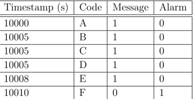
Now, we show the structure of both the event log file and the UPScale, which were provided by the company that collaborated to this thesis. The event log file is a table in which columns represent the device that generate an event and rows represent the occurrences of those events. An example of the event log file is reported in Table 3.1, A, B, C, D, E, F are the events that occur during the execution of the system. For instance, the event A is generated by the device 1, the events B and C are generated by the devices 1 and 5 and they occur at the same time, namely 2.

Devices Time 01 02 05 06 1 A 2 B C 3 D 4 E F

Table 3.1: This table shows how the event log file is structured.

When two events occur in the same row but with different columns it means that they are happening at the same time but from different devices. The time column represents the succession of the events without giving us information about the amount of time between these events. By considering the example introduced before, the events A and B may happen approxi-mately at the same time, in an hour, or in different days. In the event log file, every event is written as a plain string that contains a set of attributes. Table 3.2 shows how the event A of the example could appear.

(42)

01: 09.05.17 14:18:38 c=1202 s=miL- MAINS RECT. FAULT

Table 3.2: This table shows how an UPS reports an event.

We can already identify a set of information related to each event: • Device Number: reported at the beginning of each string that is the

same number of the column where the event appears.

• Date: represents the instant of time at which an event is written in the log file. That different with respect to the instant of time at which the event is generated, we describe in Section 5.2.3 how resolve this potential problem.

• Event information: represents a description of the event that has been generated. In the event log file, an event is described by both a code and a text description. The code is usually number between 1000 and 9999, in some cases it is composed by a letter followed by 3 numbers, for instance A101. The text description is composed of few words, for instance MAINS RCT CTRL ERROR.

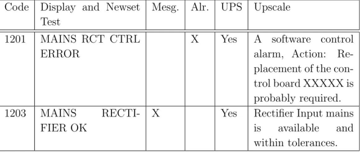
The second file provided by the company and used in our analysis is the UP-Scale. When a failure occurs, this file contains all the information regarding that failure mode. The customer service uses UPScale as the reference guide to maintain and repair a UPS. The main structure of this file is reported in Table 3.3 where we show the events with code 1201 and 1203.

Code Display and Newset Test

Mesg. Alr. UPS Upscale

1201 MAINS RCT CTRL

ERROR

X Yes A software control

alarm, Action: Re-placement of the con-trol board XXXXX is probably required.

1203 MAINS

RECTI-FIER OK

X Yes Rectifier Input mains

is available and within tolerances.

(43)

The first two columns are used to identify an event by including both a code and a text description. Subsequently, there are Boolean information about the event type (message or alarm), an event cannot belong to both the categories. In the end, there is a natural language description on what to do to repair the UPS in case of fail. As we see from the data, when an alarm occurs, there is an action or a set of actions to take in order to repair the device. On the other hand, when a message occurs it is reported the reason of that message without any maintenance strategy. The event type is a crucial information for our model because it is the only way we have to separate the non-crucial fails and critical faults.

3.4 Goals and requirements

As already illustrated, UPS systems are fundamental to many business com-panies, in order to avoid that if an unexpected power disruption causes in-juries, fatalities, data loss, or serious business disruption. Usually, in the contracts between the UPS providers and clients, there may be fines when the UPS system violates its correct behaviour. In order to know the failure mode that could be reached by a UPS, a model capable of predicting its fu-ture evolution is needed. Thanks to this prediction it is possible to improve the quality and the dependability of the UPS system in terms of time to repair and costs from both provider and consumer sides.

A model that relates messages, alarms and maintenance strategies could be used by the provider to understand on which sub-component the fails occurs. Furthermore, given the probability of every change of state, it is possible to inform the use of different maintenance strategies, by dynamically providing the most probable sub-component to change. The model can also be used to evaluate the maximum utility of a replace versus a repair strategy. A model capable of predicting the behaviour of the faults could also be used by the sales support in order to demonstrate how that UPS system can perform well with respect to competitors. Thus, an application able to compute and display the models is required.

Obviously, since the application will be used by different sectors inside a company (technicians, engineers, customer service, maintenance service), an easy to use user interface is needed to set the parameters. Moreover, the resulting model should be shown to the user easily. Another fundamental requirement of this kind of application regards the integration with existing

(44)

processes and the embedding of domain knowledge and company-specific information.

3.5 Formalising the problem setting

Before creating a model, we must understand how to pre-process the data provided, in order to be efficiently read by a computer. Moreover, we must analyse their distribution over different factors. We conduct this analysis by considering the day, the device, and the order of the events in the event log file. A complete description of the work done on the data is reported in Chapter 4. After this analysis, the model we decided to build relates the information provided in the event log file and in the UPScale file. Starting from the event log file, we create a series of chains that associate a message with the following until an alarm occurs. Based on the UPScale file we also make an association between an alarm and a set of maintenance strategies.

3.5.1 Model selection

We choose to develop a model of the system by considering Markov chains and hidden Markov models. We have already highlighted their points of strength in Section 2.3 but, in our problem, the data provided by the company are not enough to compute a real probability of the events. Furthermore, the service log file is missing and we cannot give a real probability on the association of a maintenance action with an alarm. We will assume in Section 5.6.2 how the service log file could be used.

In general, while it is obvious that a complex model describes better a system, a simple model is easier to understand, build, and maintain. In these cases the best solution consists of picking up the easiest model that is “good enough” to describe the system. We decide to study and implement a Markov chain model and consider that the states are fully observable. The main reason is the possibility to understand better the behaviour of the Markov chain model with respect to the hidden Markov model. We describe at the end of the Chapter 5 the hidden Markov models may be used to create a model with better prediction capability.

(45)

3.5.2 message/alarm association

To be as general as possible, the model can be built by taking into account four parameters. The first is the device number: we can choose to create the model by considering only a subset of devices. This allows us to consider the specific set of states coming from that specific set of devices, this parameter is useful in case we want to model only a portion of the entire system. The second parameter that can be considered for building the model is the interval of time of interest. This parameter selects a subset of events, from the entire set, from which we will build the model. This parameter allows us to extract and analyse the behaviour of the system during a particular time interval. In fact, the first two parameters are used to obtain a subset of events from the event log file to train the model.

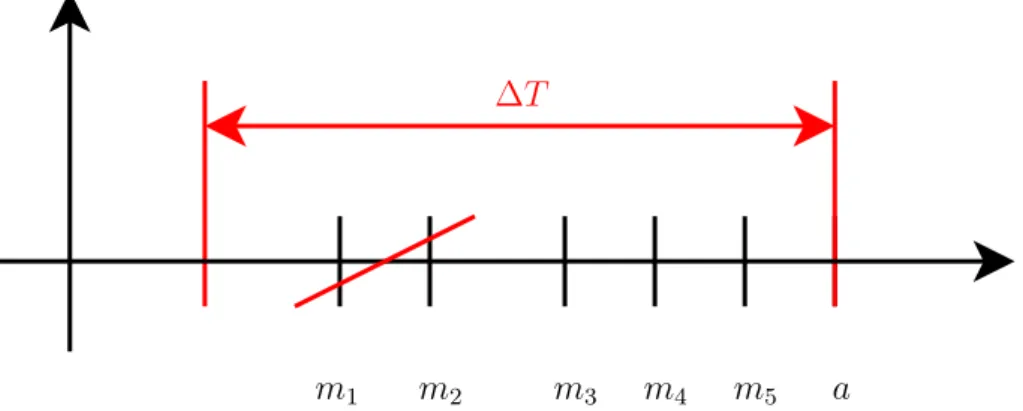
The following two parameters of the model are used to define how the events are associated with each other. The third parameter that is used to build the chains of the model is the delta time (∆T ) between the first event of the chain and the last. In our analysis we build the chains composed of a series of ordered messages ending with an alarm, in Section 5.2 we discuss this choice. By considering Figure 3.1, the messages m1 and m2are not inside

the time window ∆T . The sequence generated from this event log file with the given ∆T contains three messages and one alarm: Q = m3, m4, m5, a1.

m1 m2 m3 m4 m5 a

∆T

Figure 3.1: The figure shows how the ∆T works in the event log file.

To define the sequences, the fourth parameter that we consider is the chain length (N), defined as the number of messages inside the time window. This parameter is needed because it may happen that inside a ∆T we can have too many messages and it is reasonable to assume that not all these messages are associated with that alarm. So, we define N that is the maxi-mum number of the messages to be considered in a sequence before an alarm. As shown in Figure 3.2 with N = 3 it is possible to say that m1 and m2 are

(46)

not associated with a because there already are at least N messages between them and a. The result of these operations creates a sequence of events that

m1 m3 m5 a

∆T

m4

m2

Figure 3.2: The figure shows how the chain length parameter (N ) works when a sequence is too long.

ends with an alarm. The formal definition of a sequence is reported in the formulas below:

Q = (q1, q2, ..., qN, a) (3.1a)

where a ∈ A ∧ q1...N ∈ M (3.1b)

T (a) − T (q1) ≤ ∆T (3.1c)

A is the set of alarms, M is the set of messages, and T (k) represent the instant of time of the event k. A detailed description of how these parameters are used is shown in Chapter 5.

3.5.3 Alarm/maintenance actions association

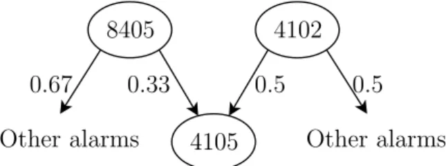
Based on the UPScale file we can add more information to each sequence. An alarm a can be associated with a set of different maintenance actions f1, f2.

It means that for each alarm we have a set of possible actions to do on the UPS in order to restore it. These associations are extracted from the UPScale and appended at the end of the chains defined in the previous Section. Let us introduce the example in Figure 3.3 where we have a1 associated with f1

(47)

a1 a2

f1 f2 f3

Figure 3.3: The figure shows how the associations between alarms a1, a2 and

mainte-nance actions f1, f2, f3 look like.

In order to be as accurate as possible, there are two ways to verify these associations. In the first case, every association should be checked by tech-nical experts, the result will be composed of a static result of which are the real associations. In the second case, the associations could be extracted automatically from historical data, the result will be dynamic and capable of capturing the hidden dependencies between alarms and maintenance actions unknown by the technical experts.

The last element we introduce in the chains is an initial state (init) rep-resenting a condition in which we have not received messages or alarms yet. After this analysis, the series of complete chains are composed by four dif-ferent elements. The first is the init state, after that it continues with the sequence discovered in the previous process Q = (m1, m2, m3, a1). At the

end of the chain, we find the maintenance strategy (f1, f2, f3) to repair the

UPS that generates that alarm. In general, the probability to reach an alarm state can be higher or lower than that of reaching another alarm state. This probability depends on the data contained in the event log file. The example below shows how a chain is represented in an informal graph and with formal equations:

init q1 q2 qN a f

Figure 3.4: By using the graph representation, the figure shows an example of a chain.

R = (init, Q, fj) (3.2a)

(48)

a ∈ A ∧ (3.2c)

q1, q2, ..., qN ∈ M ∧ (3.2d)

T (a) − T (q1) ≤ ∆T ∧ (3.2e)

f ∈ F (3.2f)

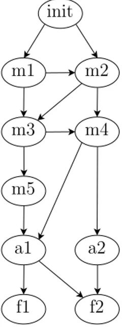
In Equations 3.2 we formally define a chain. F is the set of maintenance actions. Obviously starting from the initial state, the chains can share some messages, alarms, or maintenance actions. We can identify a set of messages that can occur in the first place, others that occur in the second and so on. Instead of representing the model by using separate chains we can use a graph. For instance, we can express the chains below by using the chart in Figure 3.5: R1 = (init, m1, m3, m4, a1, f1) (3.3a) R2 = (init, m2, m3, m5, a1, f2) (3.3b) R3 = (init, m1, m2, m4, a2, f1) (3.3c) init m1 m2 m3 m4 m5 a1 a2 f1 f2

Figure 3.5: By using the graph representation, the figure shows an example of three chains whose have shared states.

(49)

3.6 Libraries and software used

We have started the work by using Microsoft Excel to extract the attributes and to extract, from the file provided, all the useful information. We devel-oped our application using Python because of the presence of a large number of standard libraries. Furthermore, Python meets our integration and porta-bility requirements. The application relies on different libraries, the first is called “Pandas” [33] and it offers data structures and operations for manip-ulating numerical tables and time series efficiently. In our case, Pandas is used to import the files and to handle all the data we have. To show the results we used “Networkx” [34] and “Graphviz” [35], two libraries for study-ing and creatstudy-ing graphs and networks. The application is easy to use thanks to “Tkinter” [36], the standard Graphical User Interface of Python.

(50)

(51)

Chapter 4 Preprocessing and data analysis

This chapter illustrates the preliminary steps performed on the provided files in order to evaluate and understand the data we have. In Section 4.1 we extract all the information provided by the files. In Section 4.2 we analyse the information extracted in order to find patterns and distributions of the data. In Section 4.3 we introduce the dot notation to address events and attributes. In this work, the preprocessing and data analysis part is essential because we have a small dataset so we must understand thoroughly the information contained in the input files.

4.1 Preprocessing of the data

The first file provided by the company, as mentioned in Section 3.3, is com-posed of plain strings and it cannot be used to build the models. In the preprocessing phase, we make this file understandable from a computer by extracting as much information as we can and by inserting the information in a new .xls file. In this table, we can divide the columns in three logical groups:

• Id: it describes the number of the device that generates the event. • Date and hour: they describe the instant of time in which the event

occurred.

• C, S, and error: they describe the type of event by providing a code and a text description. The S attribute is unusable because, for

(52)

each event, it always contains the same value (miL−) so it will not be considered in this analysis.

Beyond these fields, in the resulting table that is the input data to build the models, we add the temp attribute that describes the order of the events. In the event log file there can be two or more events happening at the same time for two or more different devices. The temp attribute aims at keeping track of that by providing the same number when two events are on the same row of the input file. Considering, for instance, Table 3.1, introduced in the previous chapter, the events B and C have the same number in the temp attribute.

For some lines of the input file, the strings are bold and coloured in red or green. To keep track also of this information we add two further attributes: • Colour: it can be B when the input string is coloured in black, G when

green, and R when red.

• Bold: this attribute can assume the values B when the string is written in bold or N when it is not.

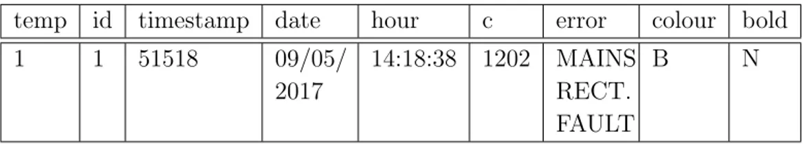
The next step of the preprocessing consists of converting the dates and hours to a standard format in order to make the computation of the time inter-vals easy. We have also to provide some considerations about the C (code) attribute because different codes may represent the same event in the sys-tem. In these specific situations we use the same event code. There are also some codes containing letters instead of only numbers, and we convert them to a number. By considering the Table 3.2 as input file, the result of the preprocessing phase is reported in the Table 4.1.

temp id timestamp date hour c error colour bold

1 1 51518 09/05/ 2017 14:18:38 1202 MAINS RECT. FAULT B N

Table 4.1: This table shows the information extracted from the event log file of Table 3.2.

From the second file, called UPScale and defined in Section 3.3, we man-ually extract information about the event type and the maintenance actions

(53)

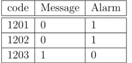
needed to repair a device. The result of this extraction consists of two sep-arate files. The first makes an association between event code and its type. This association is merged in the event log file in order to have a unique source of data. Starting from the Table 3.3 of the Section 3.3, the resulting association between event code and type is shown in the Table 4.2.

code Message Alarm

1201 0 1

1202 0 1

1203 1 0

Table 4.2: This table shows the relation between event code and event type.

The second file relates codes and the maintenance actions by manually extracting the useful information of the Upscale attribute, defined in Section 3.3. Obviously, for each event code we can have more than one maintenance action. For example, according to the file, the alarm 1202 can be resolved by replacing the Main control board XXX (Table 4.3).

code UPScale 1202 ReplaceXXXX

Table 4.3: This table shows the relation between event code and maintenance actions.

4.2 Data analysis

After extracting all the data from the sources, in this section, we analyse them in terms of number of records and distribution over devices, dates, and time intervals. In Section 4.2.1 we analyse the number of events over days and devices. In Section 4.2.2 we compare the events of the event log file and the events of the UPScale file. In Section 4.2.3 we analyse the pattern of the event log file. In Section 4.2.4 we analyse the time between events.

4.2.1 Number of records in the event log file

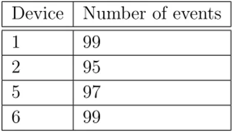
The event log file is composed of 390 events recorded by four different UPSs. We have 297 messages and 93 alarms that respectively correspond to 77% and

(54)

23% of the entire dataset. The number of events for each device is reported in the Table 4.4. As we can see they are well distributed and each device has between 95 and 99 events.

Device Number of events

1 99

2 95

5 97

6 99

Table 4.4: This table shows the number of events for each device.

The events are also equally distributed in terms of messages and alarms for each device. As we can see from Table 4.5, we have at least 70 messages and 18 alarms for each device.

Device 1 2 5 6 sum

Messages 71 70 79 77 297

Alarms 28 25 18 22 93

Table 4.5: This table shows the number of events by type for each device.

Another analysis we can do on the dataset regards the distribution of events among days. In this case, we have three different days and some differences in terms of number of events for each day. As shown by the Table 4.6, we have the 89% of the events on the 10/05, the 9% on the 11/05, and the 2% on the 9/05.

Date 9/05 10/05 11/05

Messages 3 274 20

Alarms 4 76 13

Table 4.6: This table shows the number of events by type for each day.

4.2.2 Distribution events log file vs. UPScale

Now, we analyse the distribution of events in terms of differences between the event log file and the UPScale file. By inspecting the UPScale file, a device

(55)

Figure 4.1: This figure shows the number of times in which every alarm appears in the event log file.

Figure 4.2: This figure shows the number of times in which every message appears in the event log file.

can arise 218 different events. In this set of different events, we have found 155 alarms and 63 messages. In the other and, the event log file is composed of 38 different events, 23 of them are messages, and 15 alarms. Figure 4.1 shows the distribution of alarms and Figure 4.2 represents the distribution of messages. Some events, reported in the UPScale file, are not contained in the event log file. It is trivial to exclude, in the construction of the final model, those events because it is impossible to associate them with occurrence of the event log file. We realize that in real systems may occur transitions that are not specified in the event log file but we focus our attention only on the subset of events contained in the event log file.

Moreover, the length of the used dataset is not enough to capture all the transitions and to correctly define how is likely that a transition occurs. We model only the transition contained in the data. This means that, the

A Markov chain model for dependability evaluation and fault prediction on UPS systems

POLITECNICO DI MILANO