A novel semi-automatic MATLAB tool for the analysis of the patient-specific aortic valve cusps biomechanics using solid elements

(1)

Politecnico di Milano

SCUOLA DI INGEGNERIA INDUSTRIALE E DELL’INFORMAZIONE Corso di Laurea Magistrale in Ingegneria Biomedica

Tesi di Laurea Magistrale

A novel semi-automatic MATLAB tool for the analysis of the

patient-specific aortic valve cusps biomechanics using solid

elements

Candidati: Giovanni Rossini Matricola 824381 Marco Sabbatini Matricola 822713 Relatore:

Prof. Alberto Cesare Redaelli

Correlatori:

Ing. Emiliano Votta Ing. Francesco Sturla

(2)

La somma dei due, l’1 + 1 degli uomini dà un risultato superiore a 2, certe volte. Succede quando la cordata è affiatata. Succede in montagna quando i cervelli pensano insieme e i polmoni respirano allo stesso ritmo.

(3)

1 Abstract

Introduction

The aortic root (AR) is the functional and anatomical unit connecting the outlet of left ventricle to the ascending aorta. It includes the aortic valve (AV), the Valsalva sinuses, the aortic annulus, the sino-tubular junction (STJ), the interleaflets triangles and the proximal ascending aorta.

With the aim to better understand AR structural mechanics, different approaches are available in the scientific literature. These involve the following main steps: the defi-nition of AR geometry, the discretization of the reconstructed domain, the consistency between AR geometry and loading conditions, and the modeling of the mechanical response of AR tissues.

The quantitative reconstruction of AR geometry is the first step towards the imple-mentation of a structural model. In terms of geometrical realism, three generations of models can be identified in the literature: first, models relying on a very simple and idealized geometry, typically based on the assumption of i) identical sinus-leaflet unit, ii) plane-symmetry of each unit, and iii) straight longitudinal axis of the AR bulb and of the proximal ascending aorta, as well exemplified by the work of Gyaneshwar [15]. Second, models that still made use of idealized geometrical paradigms, but used measurements from in vivo images to set the dimensions of AR substructures, as re-poted in the work published by Conti et al. [12]. Third, models based on the complete 3D reconstruction of patient-specific anatomies through the segmentation of clinical images, as presented in the work of Chandran et al. [10]. These models represent the current state of the art.

The discretization of the geometry is the second main step. For the aortic wall and the aortic valve, both topologically 2D shell elements and 3D elements are used in literature. However, these two options are not fully equivalent, in particular when dis-critizing the aortic valve: using 3D elements implies more complex meshing algorithms and higher computational expense, but also allows for more realistic simulations of valve dynamics and for accounting for the multi-layer structure of the valve leaflets. When modeling AR tissues mechanical properties, many studies assumed for

(6)

simplic-ity a linear, elastic, isotropic behavior for all of the aortic root structures. This may be sufficiently appropriate for the AR wall, which shows a non-marked anisotropy, as discussed in the work of Gundiah [18], but for the valvular structures a more complex formulation is mandatory to take into account both the anisotropy and the hyperelas-ticity of the tissue, as shown in Chandran [10] and Conti [12].

Analysing AR throughout the cardiac cycle also requires to define the initial loading state to be applied to the reconstructured geometry. Several studies usually assume the end-diastolic configuration of the AR as the initial one, and neglect the stresses acting on the in vivo AR in this configuration; in some cases the loading of the aortic wall is completely neglected [24], in other cases the aortic pressure imposed in the simulations ranges from 0 to 40 mmHg, assuming an 80 mmHg off-set represented by the end-diastolic pressure, underestimating aortic wall stresses [26]. These approaches made the modeled loading conditions inconsistent with the modeled AR geometry; the only exception was provided by Labrosse et al. [24], who estimated the unpressurized geometry of the subject-specific AR model through an iterative approach. This method was effective, but computationally very expensive, and not suitable when accounting for fine anatomical details.

In this context, a recent Masters thesis [44] developed at the Computational Biome-chanics Laboratory of the Department of Electronics, Information and Bionengineering of Politecnico di Milano, proposed a noval modelling approach. The latter recon-structed the AR geometry from cMRI, made use of a single layer of shell elements to discretize the geometry of aortic valve leaflets, and computed the pre-stress field associated to the loads acting on the reconstructed geometry through a single step procedure.

The principal aim and novelty of the present work is the design, implementation, and tesing of a semi-automated algorithm to generate patient-specific image-based aortic root finite element models completely discretized with hexahedral elements, including the possibility to set the space-dependent patterns of leaflets thickness. Such algorithm had to be integrated in a automated pipeline allowing for the computation of the AV pre-stresses and for the subsequent simulation of AR structural response throughout the cardiac cycle.

(7)

In order to test the impact of this novel approach, this method was applied to a small cohort of subjects and its results were compared to the ones yielded by models dis-cretized using AV leaflets either with shell elements or uniformely thick solid elements.

Material and Methods

The whole modelling process was handled by a Matlab© _{script that automatized the} working pipeline going from segmented images to the setting of the finite element sim-ulations to be run in the commercial explicit finite element solver ABAQUS/Explicit© (Simulia, Dessault Systemes). The entire pipeline consisted of five steps: i) acquisition of cine-cMRI data and segmentation of the AR structures in the end-diastolic frame; ii) reconstruction and discretization of AR 3D geometry; iii) definition of tissues me-chanical properties definition; iv) generation of the input files for the finite element computation of the pre-stress field acting on the AR in the reconstructed geometrical configuration; v) generation of the input files for the finite element computation of AR biomechanics throughout a cardiac cycle simulation.

The Matlab© _{script we implemented exploits the external CAD software Gambit}© (Ansys, Fluent Inc., Canonsburg, PA, USA), which is run as a batch process. Data are exchanged between Matlab© _{and Gambit}© _{through ASCII files, accordingly with the} flowchart in Figure 1. In the end-diastolic frame, patients MRI images are manually processed by in home Matlab© _{software, which allows for tracing sinuses of Valsalva,} the ascending aorta, annulus, STJ and leaflets. Each traced profile is described by a cubic spline and sampled, so to export the in plane coordinates of a set of points for each traced structure.

These raw data are automatically transformed in the 3D space and filtered in order to eliminate the noise due to manual segmentation. A network of 3D splines is then gener-ated on the aortic wall and on the leaflets, interpolating the filtered points. An optional smoothing operation was implemented in our script in order to assure a corner-free re-construction of the leaflets surface; this procedure may be necessary when the leaflets are not clearly visible during the manual tracing. Thanks to it two models of the same geometry, one with and one without the smoothing procedure, were written, ready to be imported by the CAD software Gambit©_{. The 3D surface of the each AR structure}

(8)

Figure 1: Schematic flow-chart of our automated script. Blue boxes involves Matlab© _{tools, whereas Green boxes}

(9)

is created on the profile of the splines and discretized with square shell elements; the entire procedure is handles by the CAD software Gambit©_{, which is fed with a text file} (.jou format) where all of the operations are described. The input file is automatically generated by the Matlab© _{tool. The mesh yielded by Gambit}© _{is further processed} to connect the leaflets to the aortic wall, manipulating the connectivity matrix, and to generate the solid elements. A full volume mesh for the aortic wall was created using an extrusion procedure along the node normal; instead, depending on the model the user wants to generate, the mesh of the leaflet can be of two types:

• SH model: wall made of 8-node solid elements with reduced integration (Abaqus C3D8R elements); leaflets made of 4-node shell elements (Abaqus S4 elements, with only a virtual constant shell thickness).

• 3D-HT (Homogeneous Thickness) model: wall made of C3D8R elements; leaflets made of three layers of 8-node solid elements (Abaqus C3D8 elements), obtained using a similar extrusion procedure to the one used for the wall elements but, in addition, a manipulation of the direction of the node normal was introduced in order to avoid mesh discrepancies.

• 3D-MT (Modulated Thickness) model: wall made of C3D8R elements; leaflets made of three layers of 8-node solid elements (Abaqus C3D8 elements), obtained with the same procedure of 3D-HT model; in this case, a space-dependent thick-ness value for each point of the leaflet surface was assigned taking into account the physiological variations in aortic cusp thickness [16].

Two different material formulations were used in our AR model, one for the aortic wall and another one for the valve leaflets. The mechanical response of the aortic wall was assumed linear, elastic and isotropic, with a 2 MPa Young’s modulus and a 0.45 Poisson’s ratio to reproduce the almost incompressible behavior of the real tissue [12]. AV leaflets’ tissue was described as a transversely anisotropic and hyperelastic material through the model originally proposed by Guccione and colleagues [17] to mimic the passive response of myocardial tissue. This model is based on the following strain energy function U:

U = C

2(exp Q − 1) + K(

J2_{− 1}

(10)

where C is the first constitutive parameter in MPa, J the detF , K the compressibility module and Q is formulated as follow:

Q= b1∗ tr(E) + b2∗ Ef f2 + + b3∗ (Ess2 + E 2 nn+ E 2 sn+ E 2 ns)+ + b4∗ (Enf2 + Ef n2 + Ef s2 + Esf2 ) (2) The terms Eij are the components of the Green-Lagrange strain tensor and b1, b2, b3 and b4 are the other constitutive parameters; so the model just needs six parameters (C, b1, b2, b3, b4, K) to completely describe the material properties. These were identified based on experimental data from biaxial tensile tests by Billiar et al. [3] [4]. The consistutive model was implemented into a VUANISOHYPER_STRAIN subroutine for ABAQUS/Explicit©_.

A density equal to 11 g/cm3_{, 10-fold the physiological value [15], was assumed for all} AR’s tissue taking into account the inertia related to the presence of the blood. The initial configuration of the AR was defined at early systole, when AV leaflets are approximately unloaded. Hence, cMRI data in the first systolilc frame were used to define AR reference geometry. The finite element computation of the pre-stress field acting on the AR in this configuration was required. To this aim, an iterative process was performed as described in detail in a recent work by Votta et al. [35]; briefly: the stress-free AR configuration was pressurized by applying a pressure load of 82 mmHgto the inner surface of the aorta and of the aorto-ventricular junction; then, the computed nodal displacement field was checked for the entire aortic wall; if the peak value of displacement magnitude did not exceed the in-plane resolution of cMRI, that inflated configuration was considered equivalent to real configuration related to the cMRI, and the corresponding Cauchy true stress field characterizing the aortic wall was considered the pre-stresses field to be applied when simulating AR biomechanics throughout the cardiac cycle. Otherwise, the stress-free AR configuration was updated and set equal to inflated configuration just obtained, and the pressurization simulation was performed again.

After that, the structural response of the pre-stressed AR over two consecutive cardiac cycles was computed; to this aim, physiological time-dependent ventricular and aortic pressures were applied to relevant regions of the aortic wall and a consistent trans-aortic

(11)

pressure drop to the leaflets’ surfaces.

Results

The mechanical response of the AR during the cardiac cycle was evaluated through the analysis of the stress-strain state. In particular, the attention was focused on the leaflet belly region, the most stressed area of the cusps, at diastolic peak, the moment showing the highest stress values. In SH models, the stress distribution (Figure 2) showed a patchy distribution, and a clear separation between the belly region and the coaptation area could not be detected. Conversely, in the solid elements models (3D-HT, 3D-MT) the distribution was much more regular. In addition, calculated stress values proved the strong impact of the thickness modulation procedure on the 3D-MT model biomechanichs; in particular, max principal, radial and circumferential stresses were notably increased in the thinned belly region. For all subjects, for example, the circumferential stress values averaged over the three leaflets’ bellies for the 3D-MT models are more than 4-fold as compared to the corresponding values for 3D-HT models, and more than 2-fold as compared to the corresponding value for SH models (Table 1).

(12)

Figure 2: Max principal stress computed at the diastolic peak for the AR1 subject (left column), AR2 subject (central column), AR3 subject (right column). First line: max principal stress distribution on the mid surface of the three SH models. Second line: max principal stress distribution on the mid solid level of the three 3D-HT models. Third line: max principal stress distribution on the mid solid level of the three 3D-MT models. Fourth line: max principal stress distribution on the mid solid level of the three 3D-MT models in a different stress scale to better highlight the stress distribution in these models.

subject AR1 subject AR2 subject AR3

SH 3D-HT 3D-MT SH 3D-HT 3D-MT SH 3D-HT 3D-MT

σmax_principal [MPa] 0.407 0.204 0.857 0.332 0.176 0.712 0.414 0.210 1.048

σcirc[MPa] 0.362 0.200 0.829 0.277 0.173 0.709 0.353 0.208 1.037

σrad[MPa] 0.137 0.065 0.245 0.149 0.076 0.286 0.172 0.092 0.336

Table 1: Average max principal, circumferential and radial stress across the three leaflet (LC, RC and NC) for all subjects. σmax_principal= averaged max principal stress. σcirc= averaged circumferential stress. σrad = averaged

radial stress.

(13)

distri-bution across the leaflet thickenss, the circumferential and radial stress were evaluated across the leaflet surface in all the models. The measures were performed at the dias-tolic peak in three different points (A, B, C) of the left-coronary leaflet (Figure 3.a); at each location, the stress values were extracted on the aortic side, on the ventricular side and at the mid-section of the leaflet. This three positions were geometrically dis-tinct in models using solid elements, and corresponded to different integration points in models using shell elements.

Figure 3: a) schematic longitudinal section representing the locations (green points) across the leaflet surface in which the stresses were evaluated. b) subject AR1; circumferential stress(σcirc) and radial stress (σrad) within the cross

section of the LC leaflet at diastolic peak. V side = ventricular side of the leaflet surface. mid section = middle section of the leaflet surface. A side = aortic side of the leaflet surface.

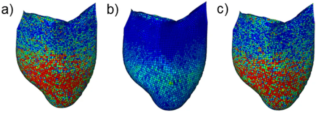
Figure 4: Stress distribution on the V side (a), mid-section (b) and A side (c) for the SH model of the AR1 LC leaflet.

The most evident stress gradient through the leaflet thickness was obtained at location A and B, consistently with the marked local curvature (Figure 3.b). Of note, in SH models the V side and the A side exhibited an even more patchy and noisy stress distribution as compared to the mid section (Figure 4); hence, side-to-side stress

(14)

variations are not reliable in these models, and only results for 3D-HT and 3D-MT models can be considered reliable.

Conclusions

As already said, the principal aim and novelty of the present work is the design, im-plementation, and testing of a semi-automated algorithm to generate patient-specific image-based aortic root finite element models completely discretized with hexahedral elements, including the possibility to set the space-dependent patterns of leaflets thick-ness. Such algorithm had to be integrated in a automated pipeline allowing for the computation of the AV pre-stresses and for the subsequent simulation of AR structural response throughout the cardiac cycle. A particular attention was payed to the analysis of stress and strain patterns in the leaflets belly, which is the region that experiences the highest stress and strain values during the cardiac cycle, and was mechanics strongly depends on its thickness. Computed results highlighted that the use of solid elements indeed lead to a more reliable quantification of leaflet stresses and of the associated gradient through the leaflet thickness. Moreover, it was evident that leafelt stresses strongly depend on the local leaflet thickness, thus suggesting that in the context of patient-specific modeling a reliable quantification of the patient-specific tissue thickness distribution should be mandatory. Hence, the most important improvement concerns the imaging technique; as already said, cMRI cannot provide any information about the patient leaflets’ thickness distribution and a higher resolution imaging technique, e.g. 3D ultrasound imaging, have to be considered in order to be able to trace also the patient-specific tissue thickness distribution. In addition, other modelling improve-ment could be impleimprove-mented in order to overcome the following limitations: i) a more complex extrusion function could be implemented for the aortic wall, in order to obtain a thickness value closer to the real one; ii) a more realistic material formulation should be implemented for the wall elements, taking into account its anisotropy; iii) different material formulations for the three layers of the leaflet could be defined taking into account the high differences among the stress-strain curves of the the three laminae of the leaflet [30].

(15)

2 Sommario

Introduzione

La radice aortica (AR) è l’unità funzionale ed anatomica che connette l’uscita del ven-tricolo sinistro all’aorta ascendente; in particolare contiene i lembi della valvola aortica (AV), i seni di Valsalva, l’annulus aortico, la giunzione sino-tubulare (STJ), i triangoli interleaflet e il tratto prossimale di aorta ascendente.

Con lo scopo di comprendere al meglio ogni aspetto dell’analisi della meccanica della AR, diversi approcci sono stati sviluppati in letteratura analizzando i seguenti aspetti: definizione della geometria della AR, discretizzazione del dominio ricostruito, consi-stenza tra la geometria della AR e condizioni di carico, e modellazione della risposta meccanica dei tessuti della AR.

La ricostruzione quantitativa della geometria della AR rappresenta il primo step nel-l’implementazione di un modello strutturale. Per quanto concerne il realismo geome-trico, in letteratura possono essere individuate tre generazioni successive di modelli: dapprima questi si basavano su una geometria molto semplice e idealizzata derivante dalle seguenti assunzioni di i) unità seni-lembi identiche fra loro, ii) simmetria planare di ogni unità, e iii) asse longitudinale dritto per i seni aortici e l’aorta prossimale, di cui si può avere un esempio nel lavoro di Gyaneshwar [15]. I modelli sviluppati in seguito, pur usando ancora geometrie paradigmatiche e idealizzate,utilizzavano misure in vivo per dimensionare le varie strutture della AR, come visto nel lavoro di Conti [12]. La terza e più attuale generazione comprende modelli geometrici basati sulla ricostruzione 3D completa di anatomie paziente-specifico attraverso la segmentazione di immagini cliniche come presentato nel lavoro di Chandran [10].

La discretizzazione della geometria rappresenta il secondo importante step. Parete e valvola aortica vengono discretizzate sia con elementi 2D shell che con solidi 3D. Questi due tipi di soluzioni non sono del tutto equivalenti, soprattuto per quanto riguarda la discretizzazione della valvola aortica: utilizzare elementi 3D comporta maggiori costi computazionali e un più complesso algoritmo di meshing, d’altro canto però permette di effettuare simulazioni della dinamica valvolare più realistiche e di ottenere strutture valvolari multi-strato.

(16)

Per quanto riguarda la definizione delle proprietà del materiale, molti studi assumeva-no per semplicità un comportamento lineare elastico e isotropo per tutte le strutture della AR. Questo metodo può risultare sufficientemente adatto per quanto riguarda la parete aortica, che non mostra un livello di anisotropia estremamente marcato [18], mentre una fomulazione più complessa è richiesta per modellare i lembi valvolari, dove è necessario tener conto sia dell’anisotropia che dell’iperelasticità, come fatto nei lavori di Chandran [10] e Conti [12].

L’analisi della dinamica della AR durante il ciclo cardiaco richiede anche la definizione di uno stato iniziale di sforzo da applicare al geometria 3D ricostruita e discretizzata. Diversi studi assumono la configurazione della AR a fine diastole come configurazione iniziale, trascurando gli sforzi agenti sulla struttura in vivo. In altri lavori invece la pressione imposta durante le simulazioni di ciclo cardiaco variava tra 0 a 40 mmHg, as-sumendo una pressione di off-set pari a 80 mmHg rapprentativa dalla pressione di fine diastole, con la conseguente sottostima delle condizioni di carico della parete aortica [26]. Questi approcci rendono le condizioni di carico inconsistenti con la geometria del-la AR ricostruita, con del-la sodel-la eccezione del del-lavoro di Labrosse [24], in cui del-la geometria paziente-specifico della AR non pressurizzata è stata modificata iterativamente. Que-sto metodo si è rivelato efficace, ma molto pesante dal punto di vista computazionale e non adatto se si vuole tenere in conto di un alto dettaglio anatomico.

Il principale scopo ed elemento di novità del presente lavoro riguarda la progettazio-ne, l’implementazione e il test di un algoritmo semi-automatico per la generazione di modelli agli elementi finiti paziente-specifico di AR basati su immagini cMRI e comple-tamente discretizzati con elementi solidi esaedri, includendo la possibilità di ottenere una modulazione dello spessore dei lembi valvolari. Tale algoritmo è stato poi integrato in un processamento dei dati automatizzato atto alla elaborazione dei pre-stress e alla successiva valutazione della risposta strutturale della AR lungo tutto il ciclo cardiaco. Con lo scopo di analizzare l’efficacia di questo nuovo approccio modellistico, tale me-todo è stato applicato ad una piccola gamma di soggetti e i corrispettivi risultati sono stati poi comparati con quelli ottenuti su modelli con lembi valvolari discretizzati sia con elementi shell che con elementi solidi esaedri a spessore omogeneo.

(17)

Materiali e Metodi

L’intero processo di modellizzazione viene gestito da Matlab© _{(The MathWorks,} Na-tick, Massachusetts, USA) che rende automatico tutto il processamento dei dati, dalla segmentazione delle immagini al settaggio delle simulazioni agli elementi finiti che ven-gono poi eseguite mediante il solutore esplicito ABAQUS/Explicit© _{(Simulia, Dessault} Systemes). L’intera catena di processi è composta da cinque fasi: i) acquisizione dei dati dalle immagini cMRI e segmentazione delle strutture della AR all’istante di fine diastole; ii) ricostruzione e discretizzazione della geometria della AR; iii) definizione delle proprietà meccaniche dei tessuti; iv) generazione del file input per la valutazione dei pre-stress agenti sulla geometria ricostruita attraverso il metodo agli elementi finiti; v) generazione del file input per la valutazione della biomeccanica della AR lungo tutto il ciclo cardiaco attraverso il metodo agli elementi finiti.

Lo script in Matlab© _{da noi implementato sfrutta il software CAD Gambit}© _(Ansys, Fluent Inc., Canonsburg, PA, USA), eseguito in batch. I dati vengono interscambia-ti tra Matlab© _{e Gambit}©_{, medianti file ASCII, coerentemente con quanto mostrato} nel diagramma di flusso in Figura 5. All’istante di fine diastole, le immagini MRI dei pazienti sono manualmente processate mediante il software Matlab©_{, che permette il} tracciamento dei seni di Valsalva, dell’aorta ascendente, dell’annulus, del STJ e dei lembi. Ogni profilo così tracciato viene poi descritto da spline cubiche e campionato, in questo modo vengono estratte le coordinate 2D del set di punti per ogni struttura tracciata.

Questi dati, ancora grezzi, sono automaticamente trasformati nello spazio 3D e filtrati in modo da eliminare eventuali rumori dovuti alla segmentazione manuale. Interpolan-do i punti filtrati, una rete di spline 3D viene generata sulla parete aortica e sui lembi. Un’opzionale procedura di "smoothing" è stata implementata nel nostro script con lo scopo di assicurare una ricostruzione dei lembi senza eccessive irregolarità geometriche. Questa procedura può risultare necessaria quando i lembi non sono chiaramente visibili durante il tracciamento manuale. Grazie a questa procedura due modelli della stessa geometria vegnono prodotti, uno con e uno senza la procedura di "smoothing", pronti per essere implementati mediante il software CAD Gambit©_{. La superfice 3D di ogni} struttura della AR viene creata sulla base del profilo delle spline e discretizzata con

(18)

Figura 5: Flow chart schematico del nostro script semi-automatico. I riquadri blu coinvolgono operazioni in Matlab©_,

(19)

elementi shell quadrati; l’intero processo viene eseguito dal software CAD Gambit©, al quale viene fornito il testo file (formato .jou) in cui sono descritte tutte le instruzioni da eseguitre. Il file input viene automaticamente generato mediante il tool di Matlab©. La mesh ottenuta mediante Gambit© _{viene successivamente processata per connettere} i lembi alla parete aortica, manipolando la matrice di connettività, e per generare gli elementi solidi. Una mesh completamente solida per la parete aortica viene creata me-diante una procedura di estrusione lungo la normale ai nodi; invece, in base al modello che si vuole generare, la mesh dei lembi può essere di due tipologie:

• modello SH: parete creata con elementi solidi a 8 nodi con integrazione ridotta (elementi C3D8R di Abaqus); i lembi vengono creati con elementi shell a 4 nodi (elementi S4 di Abaqus, con solo uno spessore virtuale costante).

• modello 3D-HT (Homogeneous Thickness): parete creata con elementi C3D8R; i lembi vengono creati con tre layer di elementi solidi a 8 nodi, ottenuti utilizzando un metodo di estrusione simile a quello usato nell’inspessimento della parete, ma, in aggiunta, una procedura di manipolazione delle direzioni delle normali ai nodi è stata introdotta per evitare eventuali discrepanze nella mesh.

• modello 3D-MT (Modulated Thickness): parete creata con elementi C3D8R; i lembi vengono creati con tre layer di elementi solidi a 8 nodi, ottenuti utilizzando lo stessa procedura del modello 3D-HT; in questo caso, con lo scopo di considerare le variazioni fisiologiche dello spessore delle cuspidi valvolari come riportato in letteratura [16], ad ogni singolo nodo della superfice del lembo viene assegnato un valore di spessore in relazione alla sua posizione all’interno della superfice del lembo stessa.

Due differenti formulazioni del comportamento del materiale sono state utilizzate nel nostro modello di AR, una per descrivere il comportamento della parete aortica e una per i lembi. La risposta meccanica della parete è stata modellata con un materiale elastico lineare e isotropo, con un modulo di Young di 2 MPa e un modulo di Poisson di 0.45; ciò ha reso possibile riprodurre il comportamento quasi incomprimibile del tessuto reale. I lembi valvolari sono stati descritti con un materiale iperelastico e trasversalmente anisotropo mediante il modello originariamente proposto da Guccione

(20)

[17] per modellizzare la risposta passiva del tessuto miocardico. Questo modello utilizza la seguente strain energy function U:

U = C

2(exp Q − 1) + K(

J2_{− 1}

2 − ln J) (3)

dove C è il primo parametro costitutivo espresso in MPa, J è il detF , K il modulo di comprimibilità e Q è formulato come segue:

Q= b1∗ tr(E) + b2∗ Ef f2 + + b3∗ (Ess2 + E 2 nn+ E 2 sn+ E 2 ns)+ + b4∗ (Enf2 + E 2 f n+ E 2 f s+ E 2 sf) (4)

I termini Eij sono le componenti del tensore delle deformazioni di Green-Lagrange, mentre b1, b2, b3 e b4 sono altri parametri costitutivi; con questo modello i sei parametri (C, b1, b2, b3, b4, K) sono sufficienti per caratterizzare completamente il materiale. Que-st’ultimi sono stati identificati sulla base dei risultati sperimentali ottenuti da test bias-siali su cuspidi naturali di Billiar e colleghi [3] [4]. Il modello costitutivo è stato poi

im-plementato in una subroutine VUANISOHYPER_STRAIN per ABAQUS/Explicit©_.

Una densità pari a 11 g/cm3_{, cioè 10 volte la densità fisiologica [15], è stata utilizzata} per tutti i tessuti della AR, in modo da tenere in conto dell’inerzia relativa alla pre-senza del sangue. La configurazione iniziale della AR è stata definita ad inizio sistole, quando i lembi valvolari possono essere considerati scarichi. Infatti, le immagini cMRI utilizzare per la ricostruzione della geometria si rifanno all’istante di inizio sistole. Il campo di pre-stress relativo a questa configurazione è stata poi acquisito mediante un processo iterativo descritto con maggiore dettaglio nel recente lavoro di Votta e colleghi [35]. Brevemente: la configurazione stress-free della AR ricostruita è stata pressuriz-zata applicando una pressione statica di 82 mmHg alla superficie interna della aorta e della giunzione tra aorta e ventricolo; in seguito è stato valutato il valore massimo dello spostamento nodale per l’intera parete aortica: se il valore di tale picco non eccedeva la risoluzione delle immagini cMRI, la configurazione pressurizzata è stata considerata equivalente alla configurazione reale e il campo di pre-stress (sforzi di Cauchy) ottenuto viene considerato corretto da applicare alla geometria prima di simulare il ciclo cardia-co cardia-completo. Diversamente, se il valore di piccardia-co di spostamento risulta maggiore della risoluzione, la configurazione stress-free viene aggiornata alla configurazione trovata e

(21)

la pressurizzazione viene effettuata nuovamente.

Una volta trovata il campo di pre-stress relativa alla configurazione acquisita dalle im-magini cMRI, la risposta strutturale del modello di AR è stata valutata su due cicli cardiaci consecutivi; a questo scopo, una curva di pressione tempo-dipendente fisiolo-gica ventricolare e una aortica sono state applicate alle rispettive regioni di interesse della parete aortica e una coerente differenza fisiologica di pressione transvalvolare è stata applicata ai lembi aortici.

Risultati

La risposta meccanica della AR nel ciclo cardiaco è stata valutata attraverso l’analisi dello stato di sforzo e deformazione. In particolare, ci si è concentrati sulla pancia dei lembi, che rappresenta la zona più sollecitata, al picco diastolico, momento in cui si registrano i maggiori valori di sforzo sui lembi. I modelli SH presentano una distri-buzione di sforzo (Figura 6) a "macchia di leopardo", e una chiara separazione tra la zona della pancia e l’area di coaptazione non può essere determinata. Contrariamente, nei modelli ad elementi solidi (3D-HT, 3D-MT) la distribuzione di sforzo è molto più regolare. Inoltre, i valori di sforzo calcolati mostravano il forte impatto della procedura di modulazione dello spessore sulla biomeccanica del modello 3D-MT; in particolare, i valori di sforzo principale massimo, circonferenziale e radiale risultato notevolmente maggiori nelle zone della pancia dove lo spessore è minore. Per tutti i soggetti in esa-me, ad esempio, il valore di sforzo circonferenziale mediato tra le pance dei tre lembi per il modello 3D-MT è più di 4 volte maggiore del corrispettivo valore nel modello 3D-HT, e più di 2 volte maggiore del corrispettivo modello SH (Tabella 2). Dato che uno degli obbiettivi principali del presente lavoro era quello di investigare la distri-buzione di sforzo lungo lo spessore del lembo per i tre modelli, sono stati valutati lo sforzo circonferenziale e radiale attraverso al superficie dei lembi. Le misure sono state effettuate al picco di diastole in tre diversi punti (A, B, C), per il lembo sinistro di ogni modello (Figura 7.a); in ogni punto, i valori di sforzo sono stati estrati sul versan-te aortico ("aortic side"), sul versanversan-te ventricolare ("ventricular side") e sulla sezione media ("mid section") del lembo.

(22)

Figura 6: Valor di sforzo principale massimo al picco diastolico per i soggetti AR1 (lato sinistro), AR2 (centro), AR3 (lato destro). Prima riga:distribuzioni dello sforzo principale massimo sulla superficie media dei tre modelli SH. Seconda riga:distribuzioni dello sforzo principale massimo sulla superficie media dei tre modelli 3D-HT. Terza riga:distribuzioni dello sforzo principale massimo sulla superficie media dei tre modelli 3D-MT. Quarta riga:distribuzioni dello sforzo principale massimo sulla superficie media dei tre modelli 3D-MT con una scala diversa, in modo da evidenziare la distribuzione di sforzo in questi modelli.

subject AR1 subject AR2 subject AR3

SH 3D-HT 3D-MT SH 3D-HT 3D-MT SH 3D-HT 3D-MT σmax_principal [MPa] 0.407 0.204 0.857 0.332 0.176 0.712 0.414 0.210 1.048 σcirc [MPa] 0.362 0.200 0.829 0.277 0.173 0.709 0.353 0.208 1.037 σrad AVG [MPa] 0.137 0.065 0.245 0.149 0.076 0.286 0.172 0.092 0.336

Tabella 2: Valori di sforzo principale massimo, circonferenziale e radiale mediati fra i tre lembi per (LC, RC e NC) ogni soggetto. σmax_principal= sforzo principale massimo medio. σcirc= sforzo circonferenziale medio. σrad= sforzo

(23)

Figura 7: a) Rappresentazione schematica di una sezione longitudinale con indicati i punti sulla superfice del lembo (punti verdi ) in cui sono stati calcolati gli sforzi. b) soggetto AR1; valori di sforzo circonferenziale (σcirc) e radiale

(σrad) lungo la sezione trasversale del lembo coronario sinistro al picco di diastole per il soggetto AR1. V side =

versante ventricolare dalla surperfice del lembo. mid section = layer medio della superfice del lembo. A side = versante aortico della superfice del lembo.

Figura 8: Distribuzione dello sforzo massimo principale sul versante ventricolare(a), sulla sezione media (b) e sul versante aortico (c) del lembo coronario sinistro del soggetto AR1.

Queste tre posizioni sono geometricamente distinte nei modelli ad elementi solidi, mentre corrispondono a tre differenti punti di integrazione nei modelli ad elementi shell (Figura 7.b). Il gradiente di sforzo più accentuato si trova nelle posizioni A e B, esattamente in corrispondenza delle zone con una più marcata curvatura (Figura 7.b). Da notare che, nei modelli SH il versante ventricolare e quello aortico presentano una distribuzione ancora più rumorosa e "a macchia di leopardo" della corrispettiva sezione media ("mid section") (Figura 8); per questo motivo, le variazioni tra una strato e l’altro del lembo non sono affidabili nei modelli SH, e un ottimo grado di affidabilità può quindi essere conferito solo ai modelli ad elementi solidi (3D-HT, 3D-MT).

(24)

Conclusioni

Come già menzionato, il principale scopo ed elemento di novità del presente lavoro riguarda la progettazione, l’implementazione e il test di un algoritmo semi-automatico per la generazione di modelli agli elementi finiti paziente-specifico di AR basati su immagini cMRI e completamente discretizzati con elementi solidi esaedri, includen-do la possibilità di ottenere una modulazione dello spessore dei lembi valvolari. Tale algoritmo è stato poi integrato in un processamento dei dati automatizzato atto alla elaborazione dei pre-stress e alla successiva valutazione della risposta strutturale della AR lungo tutto il ciclo cardiaco. Un’attenzione particolare è stata posta sull’analisi dello stato di sforzo e deformazione nella pancia dei lembi, regione dove sono presenti le maggiori sollecitazioni durante il ciclo cardiaco e che viene modificata maggiormente durante il processo di modulazione dello spessore. I risultati ottenuti hanno dimostrato che l’utilizzo di elementi solidi comporta una più affidabile quantificazione degli sforzi sul lembo e del corrispondende gradiente di sforzo lungo il suo spessore. Inoltre, è risultato evidente che gli sforzi sono fortemente dipendenti dal valore locale di spessore del lembo, suggerendo la forte necessità di introdurre una più affidabile quantificazione paziente-specifico dello spessore dei lembi. In questo contesto si inserisce un possibile miglioramento riguardante le tecniche di imaging utilizzate per l’acquisizione dei dati dal paziente: come già discusso, le immagini cMRI non permettono di ottenere alcuna informazione circa lo spessore nei lembi del paziente, dunque tecniche con una maggiore risoluzione, ad esempio il 3D ultrasound imaging, dovrebbero essere prese in conside-razione con lo scopo non solo di tracciare la posizione dei lembi, ma anche di ottenere informazioni paziente-specifico della distribuzione dei valori di spessore lungo i lembi stessi. In aggiunta, ulteriori miglioramenti possono essere apportati per superare le seguenti limitazioni: i) implementare una funzione di estrusione per i nodi della parete aortica più complessa, al fine di ottenere uno spessore più vicino a quello fisiologico; ii) utilizzare una modello costitutivo per gli elementi della parete aortica più realisti-co del semplice legame elastirealisti-co lineare isotropo, che tenga realisti-conto dell’anisotropia del tessuto vascolare; iii) implementare un legame costitutivo diverso per ciascuno dei tre strati dei lembi valvolari, così da includere nel modello le differenze nel comportamento meccanico tra le tre tunicae dei lembi valvolari [30].

(25)

3 Anatomy and Physiology

3.1 Heart anatomy and physiology

The heart is placed in the middle of the chest (anterior mediastinum), between the lungs and above diaphragm. It has a conic shape, with the apex pointing downwards and the transversal axis oriented from the right to the left and from the interior to the exterior of the chest (Figure 9).

Figure 9: Anterior view of toracic cavity with heart in the middle [39].

From a functional standpoint, the heart consists of two pulsatile volumetric pumps in series. Each of them consists of two connected chambers: the atrium, which is located superiorly, receives blood from the veins and successively moves it into the second cavity, i.e. the ventricle, which is located inferiorly and pumps blood in the arteries that supply the organs within the body. Namely, the right ventricle pumps the blood to the lungs through the pulmonary arteries, while the left ventricle pumps the blood to all of the body peripheral systems through the aorta and the corresponding

(26)

branches. The right and left hearts are separated by a wall called septum (Figure 10).

Figure 10: Anatomy of the heart [39]. Arrows indicate the direction of blood flow through the cardiac chambers.

Between each atrium and the corresponding ventricle there is an atrioventricular valve that allows for the unidirectional blood flow from the former latter. The atri-oventricular valve is called tricuspid valve (i.e. with three leaflets) and mitral valve (with two leaflets) in the right and left heart, respectively. Between each ventricle and the corresponding outgoing vessel there is a semilunar valve that guarantees the blood unidirectional flow out of the heart. The semilunar valve is called pulmonary and aortic valve in the right and left heart, respectively, owing to the artery connected to the valve. Both these valves are made of three leaflets. The opening and closure of the valves are mostly a passive phenomena driven by pressure differences between the upstream and downstream compartments separated by the valve. Based on such pressure differences, and hence on the valves’ closed or open configuration, the cardiac cycle characterizing heart function can be divided in three functional phases:

• atrial diastole: atrioventricular valves are closed to allow for the filling of the atrial with the blood coming from the pulmonary veins (left atrium) and venae

(27)

cavae (right atrium); pressure increases along with atrium filling.

• atrial systole and ventricular diastole: atrioventricular valves open under the atrial pressure and blood flows from the two atria to the two ventricles filling them completely. When the ventricular pressure exceeds the atrial pressure the atrioventricular valves close again to prevent from atrial regurgitation.

• ventricular systole: the ventricular wall undergo a fast contraction and the ven-tricular pressure increases fast (isovolumetric contraction). When pressure in the left ventricle exceeds the aortic pressure (80 mmHg) and pressure in the right ven-tricle exceeds the pulmonary artery pressure (8 mmHg) the two semilunar valves open allowing for blood ejection. Subsequently, the ventricular pressure starts to decrease to the diastolic levels and a new cardiac cycle starts.

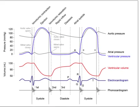
In Figure 11 the time-course of aortic pressure, ventricular volume, ventricular and atrial pressure for the left heart is plotted. At the bottom of the figure also the ECG and phonocardiogram are represented. The right heart is characterized by similar patterns, but with lower absolute values.

Figure 11: Time-dependency of aortic pressure, left atrial pressure, left ventricular pressure and left ventricular volume. Plots are synchronized with a phonocardiogram and an ECG. Values are referred to a standard healthy adult subject.

(28)

3.2 Aortic root anatomy

The aortic root is the functional and anatomical unit connecting the outlet of left ventricle to the ascending aorta and hosting the sub-structures of the aortic valve (Figure 12).

Figure 12: Anatomy of the aortic root along its long axis. The interleaflet triangle between the non- and left coronary cusp is continuous with the anterior leaflet of the mitral valve. The commissures are the coaptation lines that run parallel between the leaflets. LCC = left coronary cusp; NCC = noncoronary cusp; RCC = right coronary cusp; STJ = sino-tubular junction; MV = mitral valve [39].

The aortic wall encompassing the aortic root can be divided in two main portions: a tri-lobated bulb, consisting of the three Valsalva sinuses, and the tubular ascending aorta, which represents the most distal portion of the aortic root. The Valsalva si-nuses are called left-coronary, right-coronary and non-coronary, based on their position and on the fact that two sinuses each contain the orifice of a main arterial coronary. According to the measurements performed by Berdajs et al. [2] on 25 specimens of human aortic root under stationary flow rate conditions, each Valsalva sinus has spe-cific dimensions: the right-coronary sinus has the largest volume, which is equal to 15.6 ± 0.34 ml(mean value ± standard deviation), followed by the non-coronary sinus (1.33 ± 0.27 ml) and by the left-coronary sinus (1.04 ± 0.23 ml). The height (the exten-sion along the axial direction) of right, left and non-coronary sinus is 19.45 ± 1.91 mm, 17.45 ± 1.39 mmand 17.68 ± 1.77 mm, respectively. The thickness of the aortic wall is highly heterogeneous over different regions of the wall: in the proximal zone it ranges

(29)

from 0.60 to 1.98 mm; next to the STJ it varies between 1.82 and 2.14 mm [16]. The boundary between these two portions is called sinotubular junction (STJ). The STJ is approximately circular, with a diameter ranging from 14.4±0.4 mm during late diastole to 16.7±0.4 mm during the ejection phase [25], and it is approximately 10−15% smaller than the diameter evaluated at the sinuses base [21]. The Valsalva sinuses host the aortic valve leaflets; these insert on the aortic wall at the proximal end of the Valsalva sinuses, along a crown-shaped line called annulus. The three points at the boundary between adjacent leaflets are called commissures (Figure 13). According to the in vivo measures carried out on 10 patients by using MRI, the inter-commissures distance between the right, left and non-coronary commissure are respectively 24.2 ± 4.0 mm, 21.1 ± 3.0 mm, 22.0 ± 3.6 mm [12].

Figure 13: On the left hand panel: section of the aortic root showing its main stuctures (aortic annulus - AA - and nadir points in green, sinotubular junction - STJ - and commissures in grey. On the right hand panel: schematic representation of the aortic root.

The ideal circle connecting the three nadirs of crown-shaped annulus is called basal ring, which represents its connection between the aortic root and the left ventricle. The portions of the aortic wall delimited distally by the commissures, proximally by the basal ring, and laterally by the insertions of two adjacent leaflets are called inter-leaflets triangles (Figure 14).

(30)

Figure 14: Sketch of the aortic root opened longitudinally through the left coronary sinus, showing the interleaflet triangles (a) and the valve leaflets (b) [34].

3.2.1 Aortic valve anatomy

The aortic valve is located in close proximity of the two atrioventricular valves. In particular, the non-coronary and left-coronary leaflets of the aortic valve face the mitral valve (Figure 15).

Figure 15: Valvular plane as seen from the atrial side; valves are represented in their diastolic configuration [39]. Three aortic valve leaflets and their respective positions are clearly visible: RC leaflet (right-coronary), LC leaflet (left-coronary) and NC leaflet (non-coronary).

From the structural point of view, the aortic valve is composed by three leaflets classified as the Valsalve sinuses: left-coronary (LC), right-coronary (RC), non-coronary

(31)

(NC). In each leaflet, the line of insertion is longer than their free margin. Each leaflet covers approximately one third of aortic valve orifice. Differences in terms of leaflet extent exist, the non-coronary leaflet being wider than the coronary ones, but were reported to be not statistically significant (Table 3).

RC LC NC

Heigth [mm] 13.30 ± 0.60 13.90 ± 0.80 13.70 ± 0.40

Free margin length [mm] 33.00 ± 1.40 31.50 ± 1.40 32.70 ± 1.30

Attachment edge length [mm] 46.40 ± 2.00 47.60 ± 2.20 48.10 ± 1.60

Perimeter [mm] 79.40 ± 3.30 79.10 ± 3.50 80.80 ± 2.80

Area [mm2_] _{29.70 ± 1.70 30.90 ± 2.70 31.70 ± 1.80}

Table 3: Valve leaflets size [21].

Within each leaflet, four regions are usually identified [33] (Figure 16):

• basal region: it is located all along the insertion line of the leaflet and runs from commissure to commissure. It is characterized by an high density of fibrous collagen tissue.

• belly region: it is the central portion of the leaflet, as well as the widest and thinnest of the four regions. When inspected, this region is almost transparent. • coaptation region: the portion of the leaflet that gets in contact with the

com-plementary leaflets when the valve is closed, i.e. during ventricular diastole. • free margin: it’s the free boundary of the leaflet. The central point of this region

is characterized by the so-called nodulus of Arantius, i.e. a thicker and almost spherical anatomical feature that helps achieving the full continence of the valve during ventricular diastole.

(32)

Figure 16: Schematic representation of the four regions of an aortic valve leaflet, as seen from an anterior (left hand panel) and lateral (right hand panel) view.

The leaflets thickness is non-uniform and varies from region to region along the entire anatomy [11] (Table 4). LC & RC NC Attachment edge [mm] 1.60 1.55 Free margin [mm] 1.53 1.96 Coaptation area [mm] 0.68 − 1.29 0.68 − 1.65 Belly region [mm] 0.18 − 0.58 0.18 − 0.58

Table 4: Valve leaflets thickness values reported by Grande et al. [16].

3.2.2 Ascending aorta anatomy

The largest artery in the body, the aorta, is the main vessel of the arterial system. It originates from the left ventricle and ends in the abdomen, where it branches into the two common iliac arteries. The aorta can be divided into three main tracts: ascending aorta, aortic arch and descending aorta. The ascending aorta is 5 cm long, with a diameter of 33 mm in females and 36 mm in males [27]; the most proximal 2 cm of its the ascending aorta consist in the aortic root, and the next 3 cm consist in the tubular section. The aortic wall has a thickness ranging from 2.128 mm and 2.137 mm [16]. Being the first vessel that receives the blood ejected by the heart, the aortic wall experiences notable huge mechanical and fluid dynamic stresses.

(33)

3.3 Aortic root dynamics

In the work of Dagum et al. [13] on six adult, castrated, male sheep underwent im-plantation of miniature radiopaque markers in the aortic root, mitral annulus, and left ventricle, different dynamics and deformation processes have been shown to occur in each AR section[13]. In particular four distinct deformation modes have been found: two circumferential deformation, one on the aortic root base (annulus) and the other on the commissure level (STJ), one longitudinal deformation and a torsional deformation characterized by local shear stresses in the aortic root wall (Figure 17). In systole, the dynamics of the aortic root starts with a sudden circumferential expansion of the annu-lus and of the STJ during the isovolumetric contraction phase.While the STJ expansion is uniform, the annulus undergoes an asymmetric deformation: the expansion is larger in the left sector (11.2 ± 2.5%) and smaller in the non-coronary sector (3.2 ± 1.1%). At the same time the aortic root is stretched longitudinally. During the ejection phase the expansion of the STJ continues, whereas the annulus undergoes a non-uniform circumferential contraction: the circumferential shortening is more marked in the left and right sectors (−9.7 ± 1.5%, −9.4 ± 2.2% respectively) than in the non-coronary one (−3.9 ± 1.1%)[13]. In particular, during the first third of the ejection phase the aortic root is maximimally expanded at all levels, whereas in the last two thirds of the ejection phase the inner volume of the AR decreases slowly at first and then more and more rapidly [25]. In that phase non-homogeneous torsional stresses are present: in the left and non-coronary commissural region the torsion is clockwise (looking at the aortic root from the ascending aorta), whereas in the right commissural region the torsion is anticlockwise. In that phase no significant longitudinal deformation oc-curs. During the isovolumetric relaxation phase, the aortic root undergoes a further circumferential shrinking, both at the STJ level (symmetric) and annulus (asymmet-ric) levels. In particular the left side of the annulus feels a larger deformation than the left side (−9.9 ± 3.6%, −3.5 ± 2.1% respectively). Furthermore torsional deformation and a uniform longitudinal compression are present in the wall . In the diastolic phase the aortic root undergoes a longitudinal stretch and a circumferential expansion; shear and torsional deformations in that phase have opposite directions as compared to the ejection phase: anticlockwise in the left and non-coronary commissural regions and

(34)

clockwise in the right commissural region.

Figure 17: Aortic annular deformation of left (L), right (R), and non-coronary (NC) sectors of aortic annulus. Annular deformation throughout the cardiac cycle is shown at end of IVC (isovolumic contraction) relative to its end-diastolic configuration, at end of ejection relative to end-IVC configuration, at end of IVR (isovolumic relaxation) relative to end-ejection configuration, and at end of diastole relative to end IVR configuration.

A very important role is played by the interleaflet triangles: their dynamics is influenced by the aortic pressure and by the ventricular pressure, in particular when the upper part of the aortic root expands during systole. During systole, the expansion of the upper part of the aortic root allows the leaflets to open, while the contraction of the lower part decreases the distance they will need to cover to coapt. The rounded shape of the sinuses creates an interstice between the leaflet and the wall which allows the formation of vortexes which are very important to avoid dangerous leaflets impact on the wall. After the systolic peak those secondary flows ease the movement of the leaflets, promoting the valve closure [34][33]. The perfect synergy between the different processes described above and shown in (Figure 17) allow to maximize the ejection, optimize the transvalvular hemodynamics and ease the the leaflets movement during the cardiac cycle.

(35)

3.4 Microstructure of the aortic root

As usual in a biological environment, cardiovascular tissues are composed of connective tissues characterized by cells and extracellular matrix (ECM). The cellular part of the cardiovascular tissue is mainly composed of endothelial and muscle cells. The ECM is mainly composed by glicosamminoglycans (GAGs), two types of structural proteins, i.e. collagen and elastin, and two types of adhesive proteins, i.e. fibronectin and laminin. The microstructural properties of these macro molecules, together with their spatial organization, determine and the mechanical properties at the tissue level.

3.4.1 Ascending aorta wall structure

The proximal wall of the ascending aorta, which represents the distal part of aortic root, has three layers or tunicae, which differ from each other from both in a structural and an histological standpoint (Figure 18):

• tunica intima (I): it represents the inner layer and is 0.33 mm thick [49]. Even though it is composed of a single endothelial layer directly supported by the basal membrane, it has an important mechanical strength owing to the presence of a huge number of circumferential oriented type I and type III collagen fibers. • tunica media (M): it is the intermediate layer, separated from intima and

ad-ventitia by an elastic lamina (inner and outer respectively); it is 1.32 mm thick [49], it is composed of bundles of type I and III collagen fibers, elastin and a packed smooth muscle cell network. All of these constituents are arranged in a helicoidal pattern, which allows this tunica to bear high circumferential stress levels associated to the intraluminal pressure load.

• tunica adventitia (A): it is the outer layer of aorta and it is 0.96 mm thick [49]. Surrounded by lax connective tissue, it mainly contains fibroblasts, fibrocites, amorph substance and thick bundles of type I collagen fiber. It is perfused by the vasa vasorum, i.e. a small network of radially oriented arterial capillaries that provide nutrients and oxygen to the tunica.

(36)

Figure 18: Sketch of the main components of a healthy elastic artery composed of three layers: intima (I), media (M), adventitia (A) [41].

This complexity microstructure leads to different mechanical properties for the tu-nicae, although they all share three features: non-linearity, anisotropy characterized by a stiffer behavior in the circumferential direction as compared to the axial direction (Figure 19), and extremely high resistance to volumetric deformations. The mechanical properties of the three tunicae can be described based on the study by Holzapftel [40], even though it was focused on the wall layers of 13 specimens of human arterial coro-naries from elderly subjects (age 71±7.3 years). In that study it was observed that the tunica intima exhibits a high values of stiffness and the highest degree of anisotropy, while the adventitia has a markedly non linear response due to the progressive re-cruitment of collagen fibers during loading. The almost incompressible stress-strain behavior of the tunicae is a consequence of the strong aqueous component inside the ECM, which often leads to assumed perfect incompressibility, as shown in the works of Choung and Fung [7]. In particular, some compression tests were performed on rabbit aortae by applying a 30 kPa pressure. Results showed a volume change by to 0.5 − 1.26% associated to the ejection of liquid from the wall, thus supporting the incompressibility hypothesis.

(37)

Figure 19: Stress-strain curves for the three tunicae of coronary artery wall [40].

The superimposition of the properties of the three tunicae leads to the global me-chanical behavior of the aortic wall at the organ level, which can be described as non-linear elastic, i.e. hyperelastic, anisotropic and incompressible. The recruitment hypothesis of the collagen fibers explains the mechanical behavior of the aortic wall: initially, at low loads, only the elastin extends in order to support the stresses then, increasing the loads magnitude, the collagen fibers, aligning progressively with the stresses direction, start to sustain the loads reaching a straight configuration at high stress values. It follows that elastin allows the artery to stretch, while collagen prevents excessive distortion.

3.4.2 Aortic valve leaflets’ structure

The tissue of aortic leaflets organized into three different layers through the leaflet thickness, whose combined behavior is responsible for the peculiar characteristics of the entire leaflet: very low flexional rigidity, to guarantee a fast opening in systole, and a very high tensile strength, which allows for bearing the important high pressure differences in diastole.

(38)

Figure 20: Left hand panel : sketch of an aortic leaflet depicting the three laminae. Right hand panel : histological section of the three laminae in the aortic leaflet

The three layers show very different properties and are called laminae (Figure 20): • lamina fibrosa: it is the thickest layer (about 40% of the total leaflet thickness) [48] and covers the entire aortic surface of the leaflet. In this lamina, type I collagen fibers are orientated circumferentially (from commissure to commissure); these are folded in systole, when the tissue undergoes flexion, and stretched in diastole, when the tissue undergoes traction due to the trans-valvular pressure difference.

• lamina ventricularis: it is the layer exposed to the ventricle and it account for about 30% of the leaflet thickness [48]. It contains a dense net of collagen and elastin [42], where the radially oriented elastin fibers help reducing the radial deformation during the systole, facilitating the transvalvular blood flow.

• lamina spongiosa: it is the middle layer and account for about 30% of the total leaflet thickness. It contains many hydrated GAGs and PGs, which serve as lubricant during the relative motion of the other two layers.

The above described microstructure gives to the aortic leaflets a particular mechani-cal response with five main characteristics: non homogenous, elastic (layer structure), anisotropic (preferential directions of the collagen fibers), non-linear (collagen fiber progressive recruitment), and isochoric (water and GAGs presence). Many authors studied the mechanical response of aortic leaflets’ tissue using biaxial tests [43][29][3]. The first constitutive model of aortic valve leaflets’ tissue was formulated by Billiar

(39)

and Sacks based on load-controlled biaxial tests on human specimens [4]. The results yielded by those tests in terms of membrane tension vs. real strains in the radial and circumferential directions highlighted marked anisotropy of the tissue. In particular, the mechanical response in the circumferential directions is much stiffer than the re-sponse in the radial one (Figure 21). Indeed, the peak strain differs by more than 30% between the two directions.

Figure 21: Representative circumferential and radial stress-strain curves from a fresh and a glutaraldehyde-fixed AV cusp, which show the pronounced mechanical anisotropy of both tissues [3].

3.4.3 Aortic root wall structure

The Valsalva sinuses have an inner structure similar to the one characterizing the aor-tic wall, as they are made by three layers. The innermost one, i.e. the intima, is rich in endothelial cells in contact with blood. The middle one, i.e. the media, is full of smooth muscle cells, PGs, elastin and type II and III collagen fibers preferentially oriented in the circumferential direction. The outermost layer, i.e. the adventitia, is characterized by type I collagen fibers preferentially aligned to the axis of the ves-sel. The interleaflet triangles are mainly composed by a fibrous structure containing contractile and cytoskeleton proteins and smooth muscle cells [14]. In particular, the triangles close to the non-coronary leaflet are mostly made of fibrous tissue, whereas the triangle between the right and left leaflet is composed primarily of muscle tissue, the fibrous tissue being confined in the apex zone [38]. The annulus, containing the leaflet insertion, is a fibrous ring rich in collagen where sometimes it is possible to find elastin and demyelinated nervous terminals.

(40)

4 State of Art

4.1 Introduction

The high prevalence of cardiac diseases and to the corresponding social and economical burden has been motivating great efforts in the study of the pathophysiology of the heart and in the development of innovative clinical solutions to cardiac diseases. In particular, a massive research activity has been focusing on the aortic root (AR), either to undestand the mechanicsms underlying pathological processes (e.g. calcification of aortic valve leaflets leading to aortic stenosis, and AR aneurysm leading to aortic dis-section) or to analyze the effects of surgical and interventional procedures (e.g. valve sparing techniques, and trans-catheter aortic valve implantation).

In this context, the contionuous increase in computational power of microprocessors and in availability of parallel or distributed computing systems has boosted the exploita-tion of numerical simulaexploita-tions to aid reasearch on the AR. The latest developments in this specific type of activity merge image processing techniques and finite element or finite volume methods to quantify the structural response and the fluid dynamics, respectively, of the AR on a patient-specific basis.

In this chapter we will focus in particular on the different approaches available in the scientific literature for the analysis of AR structural mechanics. Such analysis involves five main steps: the definition of AR geometry, the consistency between AR geometry and loading conditions, the discretization of the reconstructed domain, the modeling of the mechanical response of the AR tissues, and the setting of proper boundary con-ditions to mimic kinemeatic constraints and mechanical loading due to blood pressure. Each of these steps will be discussed in the following sections.

4.2 Definition of AR geometry

The quantitative reconstruction of AR geometry is the first step towards the imple-mentation of a structural model. In terms of geometrical realism, three generations of models can be identified in the literature. The most seminal models relied on a very simple and idealized geometry, and were based on the assumption of i) identical

(41)

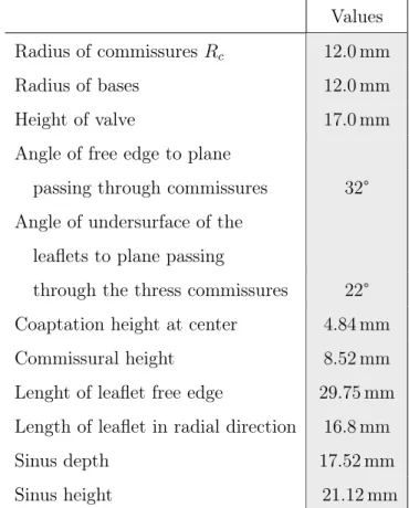
sinus-leaflet unit, ii) plane-symmetry of each unit, and iii) straight longitudinal axis of the AR bulb and of the proximal ascending aorta. This approach is well exemplified by the work of Gyaneshwar [15] where the geometry was created using the procedure illus-trated by Thubrikar in his work on the aortic valve [46]. In that work [46], he explored the design of trileaflet valves, such as the aortic valve, to ensure optimal dynamic per-formance during numerical simulations . More specifically he defined some geometric criteria to guarantee appropriate leaflet coaptation in the closed valve configuration, a proper valve height-to-diameter ratio to minimize dead space, no folds in the leaflets and minimum leaflet flexion to make the use of energy as efficient as possible. An accurate surface model of the valve meeting Thubrikar’s parameters was constructed using a computer aided design software SDRC/IDEAS© (EDS, Plano, Texas, USA), where also the thickness variation of the leaflets was incorporated. In Figure 22.a the final model is shown with substantial details of geometry reported in Table 5. The main limitation of this is that, even though it provides extremely valuable insight, the physiological variability in valve design was not properly elucidated and described and, as a result, this approach seems to be somehow too rigid to accommodate the dimen-sional variability observed in normally functioning valves.

The second generation of models still made use of idealized geometrical paradigms, but removed the aforementioned assumptions and used measurements from in vivo images to set the dimensions of AR substructures. For instance, in the the work published by Conti et al. [12] the 3D geometry was based on a paradigm that accounted for the in vivo geometrical asymmetry of the leaflet-sinus units, as well as for the curved and tilted profile of the centerline of the lumen of the AR. The dimensions of the differ-ent parts of the model were based on measuremdiffer-ents performed on cardiac magnetic resonance imaging (cMRI) performed on 10 healthy subjects, which were averaged over the 10 subjects to derive a representative model of the healthy AR. In the end-diastolic frame, the AR main geometric parameters were measured: annulus diameter, commissural positions, width of the Valsalva sinuses, and ascending aorta orientation. Each measurement was then averaged from three offline estimations by two blinded experienced operators (Table 6). Once acquired by cMRI, data were scaled so to be consistent with a 24 mm annular diameter, which is an average valve size [22], and then

(42)

were used to define each unit of the entire AR structure. To account for variations in aortic cusp thickness, different values were assigned to the thickness of the leaflets in four different regions: free margin, attachment edge, coaptation area, and belly [16] (Table 7). Furthermore, non-coronary leaflet regions were assumed to be thicker than the corresponding right and left regions [16][31]. Thickness values were assumed to be constant only for the aortic duct (2.3 mm), Valsalva sinuses (1.6 mm) and interleaflet triangles (2.3 mm) according to data reported in literature [16]. Of note, tissue thick-ness had to be defined based on data from the literature, because cMRI images did not yield any valuable information of this aspect. The final result is shown in Figure 22.b. The cMRI-derived morphological parameters used to define the 3D AR geometrical model appeared to be reliable, given the high intra and inter-operator repeatability of measurements, as well as the consistency with previous findings from the literature. However, the geometrical model was based only on measurements from 10 subjects: even though each measurement was averaged from three offline estimations by two blinded operators, and parameters’ mean values were used, more subjects should have been recruited in order to reduce random errors, limit uncertainties due to individual differences and obtain statistically sound data. Moreover, the usage of cMRI do not give the possibility to assess tissues thickness values, which were then obtained from the literature; this may be a source of uncertainty, especially with respect to leaflet stresses: leaflets indeed mainly undergo bending, and so the stresses acting on them de-pend on the third power of the thickness. Despite the limitations described above, the computed results confirmed that morphological differences between leaflet-sinus units induce important differences in stress values; thus, discarding a symmetrical design to adopt an asymmetrical one can provide more accurate stress-strain patterns.

The third and current generation of geometrical models is based on the complete 3D re-construction of patient-specific anatomies through the segmentation of clinical images. An example of such state of the art is the patient-specific AR model reconstructued from real-time 3D ultrasound images presented in the work of Chandran et al. [10]. Their aim was to create a computational tool to build AR models with tricuspid and bicuspid valve (TAV and BAV, respectively). The model was created starting from real-time 3D echocardiography (rt3DE) in the Gorman Laboratories at the University