Chaos, Fractal and Recurrence Quantification Analysis of Surface Electromyography in Muscular Dystrophy

(1)

http://dx.doi.org/10.4236/wjns.2015.54022

How to cite this paper:

Conte, E., Ware, K., Marvulli, R., Ianieri, G., Megna, M., Conte, S., Mendolicchio, L. and Pierangeli, E.

(2015) Chaos, Fractal and Recurrence Quantification Analysis of Surface Electromyography in Muscular Dystrophy. World

Journal of Neuroscience, 5, 205-257.

http://dx.doi.org/10.4236/wjns.2015.54022

Chaos, Fractal and Recurrence

Quantification Analysis of Surface

Electromyography in Muscular Dystrophy

Elio Conte

1,2*

_{, Ken Ware}

3

_{, Riccardo Marvulli}

1,4

_{, Giancarlo Ianieri}

1,4

_{, Marisa Megna}

1,4

_,

Sergio Conte

1

, Leonardo Mendolicchio

1

, Enrico Pierangeli

1

_{School of Advanced International Studies on Applied Theoretical and Non Linear Methodologies of Physics,}

Bari, Italy

2

_{Department of Basic Sciences, Neuroscience and Sense Organs, University of Bari Aldo Moro, Bari, Italy}

3

_{The International NeuroPhysics Functional Performance Institute, Robina, Queensland, Australia}

4

_{Department of Physical Medicine and Rehabilitation, University of Bari Aldo Moro, Bari, Italy}

Email:

*

elio.conte@fastwebnet.it

Received 19 May 2015; accepted 5 July 2015; published 9 July 2015

Copyright © 2015 by authors and Scientific Research Publishing Inc.

This work is licensed under the Creative Commons Attribution International License (CC BY).

http://creativecommons.org/licenses/by/4.0/

Abstract

We analyze muscular dystrophy recorded by sEMG and use standard methodologies and nonlinear

chaotic methods here including the RQA. We reach sufficient evidence that the sEMG signal

con-tains a large chaotic component. We have estimated the correlation dimension (fractal measure),

the largest Lyapunov exponent, the LZ complexity and the %Rec and %Det of the RQA

demon-strating that such indexes are able to detect the presence of repetitive hidden patterns in sEMG

which, in turn, senses the level of MU synchronization within the muscle. The results give also an

interesting methodological indication in the sense that it evidences the manner in which

nonlin-ear methods and RQA must be arranged and applied in clinical routine in order to obtain results of

clinical interest. We have studied the muscular dystrophy and evidence that the continuous

re-gime of chaotic transitions that we have in muscular mechanisms may benefit in this pathology by

the use of the NPT treatment that we have considered in detail in our previous publications.

Keywords

Chaos Analysis, Correlation Dimension, LZ Complexity, Recurrence Quantification Analysis,

Muscular Dystrophy, Chaos and Fractal Estimation by Surface Electromyography

(2)

E. Conte et al.

1. Introduction

Surface electromyography is a measure of the electrical activity associated with the contraction of muscle,

re-corded invasively using electrodes located on the surface of the skin. The obtained signal contains information

about neuromuscular and bioelectrical activity of the muscle. The surface EMG usually involves processing

techniques in time and frequency domain. They are important since giving indications about the global EMG

ac-tivity without aiming at an analysis at the single MU level. The RMS (Root Mean Square) is currently used in

time domain; instead Spectral Analysis and Amplitude enables estimating the mean and median frequency

(MDN). Finally, Muscle Activation estimations are usually performed from single differential signals to obtain

indications about the physiological processes occurring during spontaneous or sustained voluntary contractions.

Currently, we perform such kind of analysis by using the software Acknowledge 4.0 of the BioPac system

[1]

.

In addition to such standard methodological and clinical investigations, some other investigations are required,

focused on the analysis of the relationships between global variables in the sEMG and the underlying physical

processes with the finality to extract information of physiological interest from the performed global analysis of

the surface EMG signal.

Our investigations start from the view point that interference and muscle cross-talk introduce non-linearity

into the standard EMG signal. Nonlinearity, particularly in biological processes, is the constant first condition of

chaotic-deterministic biological dynamics giving origin to high complexity in time dynamics.

Generally speaking, in the last ten years in medicine as well as in biological sciences, it has become the

criti-cal issue of great interest to determine whether an observed time series of a recorded signal of

electrophysio-logical interest is purely stochastic, or deterministic nonlinear, even chaotic

[2] [3]

.

Detailed methods have been elaborated to explore the intrinsic properties of the observed phenomenon by

dis-tinguishing between nonlinear deterministic dynamics and noisy dynamics from a time series

[2] [3]

. EMG is

apparently a complex signal, highly corrupted by noise but really governed by chaotic and fractal dynamics

[4]

.

Consequently, in the attempt to obtain valuable information by EMG analysis, the methods of the nonlinear

analysis must be employed. To the best of our knowledge, recently work has been done with great consideration

in the international literature

[5]-[8]

and the finality has been determined that the real dynamics of EMG is

cha-otic and fractal also if corrupted by noise. The finality of such advanced studies is double since the nonlinear,

chaotic-deterministic methodologies would enable us to improve the understanding of the basic physiological

involved mechanisms, and, on the other hand, we could arrive to introduce new important indexes of clinical

evaluation.

Our work moves just in this direction. It aims to investigate in a detailed manner the chaotic behaviour in a

systematic fashion.

The scheme of our approach may be delineated in the following manner. Giving the sEMG, we use spectral

analysis as well as standard indexes as RMS and Muscle Activation in order to have clinical evaluation by using

the standard methodological approaches. To such standard procedures, we add nonlinear-chaotic deterministic

methods, using the standard procedure to reconstruct phase space of the given sEMG time series evaluating in

particular the Embedding Dimension, the Lyapunov Exponents, the Correlation Dimension (fractal dimension),

and LZ complexity

[2] [3]

. We also use the technique of the Generalized Mutual Information and Partial Mutual

Information for estimation of synchronization and coupling among regions of interest

[9]

. In addition, we use

the method of the Recurrence Quantification Analysis, RQA

[10]

. It is of importance to outline here that we

perform here each investigation by using surrogate data test to verify the validity of our results

[2] [3]

.

The previously mentioned and standard well-known nonlinear chaotic-deterministic methods, used as the

es-timation of Correlation Dimension, of the Largest Lyapunov Exponent, are well known to scholars so that we

will not add here further comments to evidence their importance

[2] [3]

. The use of the RQA requires instead

some further comments.

Recurrence quantification analysis (RQA) is a technique for the detection and analysis of state changes in

drifting dynamic systems without posing a priori restrictions on data size, stationarity, and statistical distribution.

This is very important for the reasons previously mentioned since EMG is often noise corrupted with hidden

MU modulating activity.

RQA is a technique of investigation whose application requires high and specific competence but its correct

application has given results that have been celebrated in a number of experimental studies in physiology

show-ing its potential ability. The important feature is that it looks at the inner structure of the examined signal.

(3)

We have also outlined here that preliminary results in application of RQA in EMG were given by Ikegawa,

Shinohara, Fukunaga, Webber and Zbilut

[11]

. These authors studied the standard variables of the RQA analysis

that are the %Rec, the %Det, the %Laminarity, the Trapping Time, the Entropy, the Max Line, and the Trend.

They tested the sensitivity of such different indexes extracted from RQA. They obtained that subtle changes in

surface EMG can be detected by using the RQA outlining thus the importance to introduce such new and

ad-vanced methodology in EMG studies. In their studies these authors were so much interested to three basic

vari-ables of the RQA that are the %Rec, the %Det and the %Lam. The profound physiological and clinical reason to

use such indexes in such new advanced EMG analysis is that the percentage of determinism (%Det) reflects the

amount of rule-obeying structure in the signal dynamic, and is strongly related to the percentage of recurrence

(%Rec), which reflects the current state of the system.

Consequently, %Rec and %Det are the most sensitive indexes of nonlinear analysis to be used in conjunction

with the spectral analysis to MU analysis. %Det reveals embedded determinisms in an apparently stochastic

signal. In addition, the %Rec estimates in detail periodicity in MU dynamics. It results that consequently we

ob-tain two indexes that are of highest valuable interest under the physiological and clinical interest. Finally,

the %Lam, added to the trapping time, will evidence the percentage of chaos-chaos transitions that we have in

the time dynamics of the considered time series in relation to MU activity. These are some basic reasons because

EMG studies conducted by RQA are so important.

Finally we have to report a final statement. The aim to use nonlinear chaotic deterministic methodologies as

well as RQA in EMG analysis is not new here. In references

[4]-[8]

, we report the indication of some previous

studies that were conducted with excellent results.

The present paper is devoted to the study of muscular dystrophy (facioscapulohumeral muscular dystrophy)

where it used the treatment NPT that is due to one of the present authors (KW). Since all the details on the basic

methods that were used have been reported by us recently in previous published papers

[9] [12]

, we invite the

reader to examine such previous papers and we will not give here further indications.

To be clear, the present paper is so long since we have to present the employed methodologies and the results

with figures and tables. Unfortunately this situation leads to here a so long work. According to the usual

proce-dure, the reader expects that the next section will be devoted to the Materials and Methods as in fact it happens

in each paper. Instead, in the next section we go directly to the results obtained presently by the application of

our nonlinear and chaotic methodologies. We will not report details on the clinical case, on the methods of

clinical investigation, on the pathogenesis and on the clinical manifestations as well as considerations on the

in-cidence rate of muscular dystrophy in population. The reason is that we have outlined in the greatest detail all

such features in our previous publications in

[9] [12] [13]

. Therefore, for shortness and in order to give the

read-ers very articulated information on the clinical profile and that we could not realize here in the due details, we

consider such papers

[9] [12] [13]

as integrating section also avoiding in this manner to overload the reader with

a lot of information and discussions. Therefore, with the following section, the reader will find directly the

re-sults of the present investigation.

2. Materials and Methods

The clinical case is explained in detail in references

[9] [12] [13]

. Since the present paper overcomes the natural

extension of a standard scientific paper, we invite the reader to consider this section as detailed in

[9] [12] [13]

.

3. The Results

In order to explain the conceptual basis of the treatment we have to recall some previously introduced statements.

We have to outline again that, according to our approach, the best way to analyze sEMG signal is by using non

linear-chaotic deterministic methods. The suggested use of such new methodologies implies obviously that the

actual nature of the explored physiological dynamics recorded by sEMG responds actually to the non linear

re-gime of chaotic dynamics and fractal behaviour.

Let us sketch briefly the question under a general profile. The use of the non linear methodologies in medicine

and in particular in physiology

[2] [3]

has offered some new results that are radically different from previous

es-tablished concepts. The basic concept in the past was as example that the body must maintain a particular

ho-meostasis, a steady state enabling the body to properly function. The basic dynamics of non linear chaotic-de-

terministic systems is based instead on the particular feature of its intrinsic variability. The results are that

(4)

exist-E. Conte et al.

ing non linear systems evidence continuous variability and any loss of variability is indicative of some sort of

pathology. Presently it is long recognized the ubiquity of chaotic and of fractal temporal dynamics in biological

mechanisms. Central to results about chaotic and fractal health relationship in physiology is the now widespread

recognition that chaotic and fractal variability means system complexity, and system complexity means a

healthy biological system with normal chaotic behaviour.

The overarching premise of the NPT (KW) treatment is that it enables to evoke transitions into and out of

system-controlled chaos, requisite for the system to reorganize itself to healthier balance.

3.1. Let Us Report Our Results before and after the Treatment

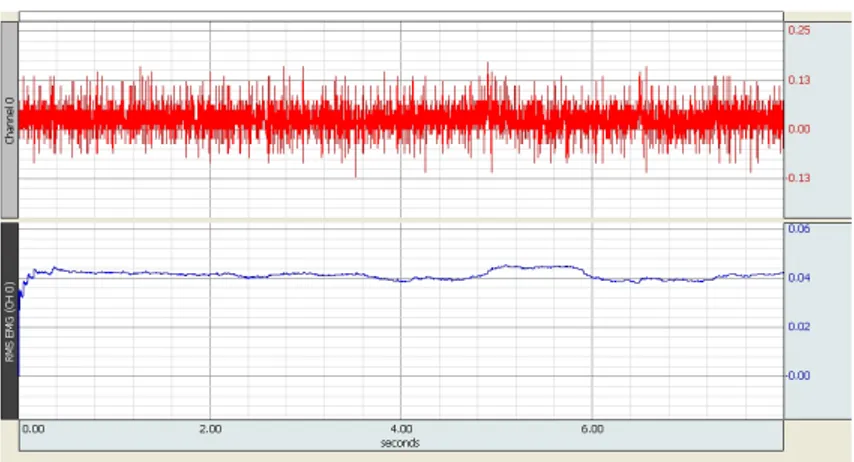
a) Standard Estimation of sEMG Signals by RMS

It is well known that by RMS (Root Mean Square) we perform modelling the process as amplitude modulated

Gaussian random process whose RMS is related to the constant force and not-fatiguing contraction. MAV

(Mean Absolute Value) is calculated by taking the average of the absolute values of the given sEMG signal

[14]

.

For RMS in Ch1 (recording on right trapeze) we obtained the mean value of 0.049 at rest before the treatment

and 0.055 after the treatment. For Ch2 (recording on the left trapeze) we had 0.084 before the treatment and

0.048 after the treatment (unities expressed in microvolts). The results are given in

Figures 1-4

.

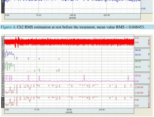
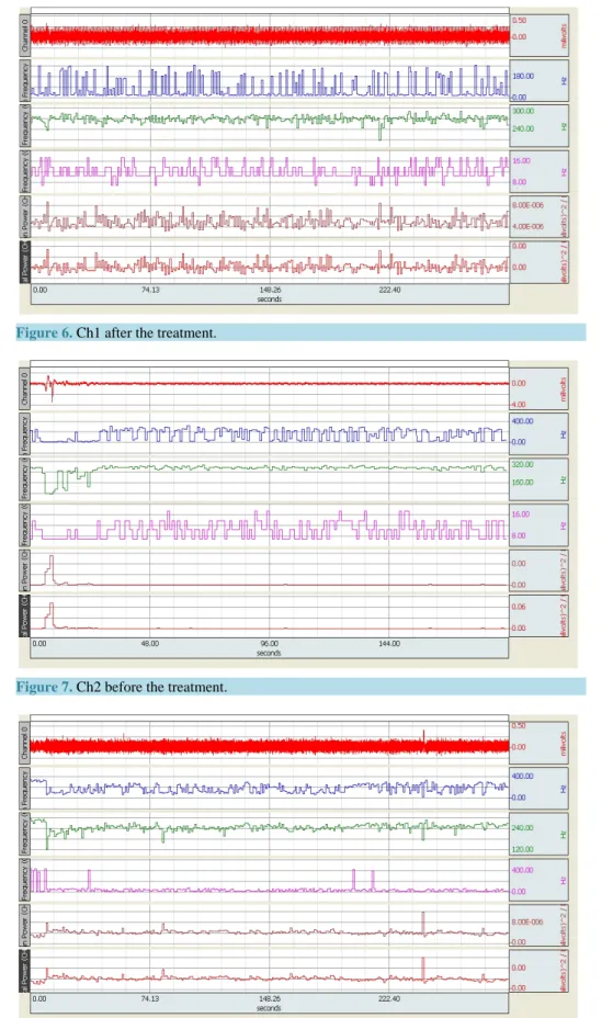
b) Frequency and Power Analysis

The next step of our analysis was represented from Frequency and Power Analysis. We estimated the Median,

Mean and Peak Frequency in Hz and the Mean and the Total Power in (milliVolts)

2

/Hz. The results are given in

Figures 5-8

. Each epoch is 1 second.

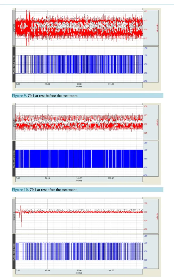
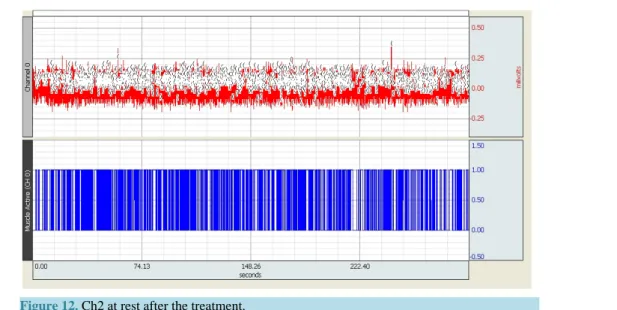
c) In

Figures 9-12

we give also the estimation of Muscle Activation.

Figure 1.

Ch1 RMS estimation at rest before the treatment, mean value RMS

= 0.048848.

Figure 2.

Ch1 RMS estimation at rest after the treatment, mean value RMS =

0.055112.

(5)

Figure 3.

Ch2 RMS estimation at rest before the treatment, mean value RMS = 0.0845668.

Figure 4.

Ch2 RMS estimation at rest before the treatment, mean value RMS = 0.048453.

(6)

E. Conte et al.

Figure 6.

Ch1 after the treatment.

Figure 7.

Ch2 before the treatment.

(7)

Figure 9.

Ch1 at rest before the treatment.

Figure 10.

Ch1 at rest after the treatment.

(8)

E. Conte et al.

Figure 12.

Ch2 at rest after the treatment.

The improvement obtained after the NPT treatment is evident at the simple inspection of the figures since

they indicate a more periodic and arranged activity on muscle activity. In addition, in Appendix we report also

the numerical results.

d) Chaos Analysis

As previously outlined, the basic finalities of this paper are to explore the NPT treatment of muscular dystro-

phy by the use of non linear analysis. as a tool that is generally employed in the clinical and biomechanical

ap-plications. Accordingly, biomedical signals can be to an extent deterministic, random or chaotic. Deterministic

signals have the characteristic of predictability. This is to say that any future time behaviour of the signal could

be predicted using some linear analysis tools. For them, mathematical tools (e.g., Fourier transform) are

com-monly used. To use Fourier transform the signal must be linear, stationary and periodic. These are crucial

re-strictions that rarely we may find in biomedical signals governed from feedback control loops. The random

sig-nals are non-deterministic in the sense that individual data points of the signal may occur in any order, with no

possibility of predictability on the future course of the signal. In this case only purely stochastic analytic tools

can be applied in electrophysiology. Finally we have chaotic signals. These signals can be viewed as a

connect-ing mesh between deterministic and unpredictable behavioural dynamics, exhibitconnect-ing time pattern that in

princi-ple is slightly predictable, non-periodic or seldom quasi-periodic (an examprinci-ple is the heart beat) but they results

strongly dependent from some control parameters and are highly sensitive to initial conditions. Dependence

from control parameters means that for some critical values of such control parameters the chaotic system

tran-sitates between so much undefined states in time giving origin to a time dynamics that becomes unpredictable

for us and thus apparently random but really revealing the signal an inner structure responding to the important

realization of the self-organization and high complexity. The system whose counterpart has a chaotic signal as

representation, reveals ability to self arrange by itself patterns of organization in its dynamics. This is of course

the basic feature of living systems. Chaotic systems are non linear open systems, responding to the external

stimuli by self-organizing each time their inner patterns and thus their time dynamics. All the considered

sys-tems in biomedicine are open syssys-tems that necessarily interact with their outside interacting syssys-tems and having

time by time the fundamental demand to responds with elasticity to the requirements arriving from the external

components. In this sense they self-organize their dynamics responding to inner and out inputs An example is

the cardiovascular system that continuously needs self-organization responding to basic requirements of inner

and output inputs and providing to heart rhythm variability, blood pressure, respiration, autonomic nervous

tem modulation, just to quote only some of the interacting components The other basic feature of chaotic

sys-tems is that they are highly sensitive to initial conditions. This is to say that each signal starts with some definite

values of its variables. Consequently, a time dynamics is generated. In chaotic systems it is sufficient that such

initial values of the variables fluctuate also at a so contained level to escape to our computational attention that

consequently a total different time dynamics is generated with new and different properties in self-organization

and structure to responds with elasticity to the requirements arriving from the external demands. Within chaos

(9)

theory, the time series that are representative of the time dynamic of the chaotic signals are represented in the

phase-space.

Embedded dimension in phase space is estimated by proper techniques that are autocorrelation method and, in

particular, the average mutual information, estimating the so called time delay. Using the criterion of the False

Nearest Neighbors we are enabled to obtain a proper representation in phase space reconstruction. Usually the

analysis arrives to reconstruct the attractor of the given chaotic system and thus representing the states, the

pat-terns and thus the subsequent transitions of the states characterizing the time dynamics of the system. Some

in-dexes may be introduced to analyze chaotic systems. In particular we evaluate the Correlation Dimenion, the

Largest Lyapunov Exponent, the Fractal dimension and LZ complexity.

Within biomedical signal processing, chaotic dynamics provide a possible explanation for the different

com-plex and erratic patterns that appear in most bio-signals and in particular in electrophysiology. Current

investi-gations span from studies of brain rhythms to heart rate variability, from blood pressure regulation to

neuro-muscular system, from breathing system to cardio-respiratory coordination including all the fields relating the

complexity of the human and animal anatomo-physiological systems.

The reason to introduce non linear methodologies and chaos analysis in EMG has been explained previously.

It is necessary to go on in further details.

The EMG and the sEMG signals are highly non-stationary signals. We know that the neuromuscular control

process works through enhancing or inhibiting feedback mechanisms implemented on neuronal circuitry

in-volving the Central Nervous System at various cortical or sub-cortical levels. In addition, we have constantly

interaction o0f acting components and the result is a non linear and highly non stationary dynamics. In these

conditions the adoption of non-linear chaotic methods is strongly required with the finality to account for the

highly non-linear behaviour of such mechanisms by muscle receptors, mechanoreceptors, nociceptors, and joint

receptors within local (spinal) and/or central sensory-motor networks. Only the use of non linear-chaotic

mechanisms may contribute to elucidate such complex dynamics since non-linear parameters reveal several

hidden mechanisms of muscle control that otherwise would be not reflected by variability of other standard

lin-ear parameters. In particular, as previously outlined, the RQA method looks at the inner structure of the given

EMG signal. The proper reconstruction of the given sEMG signal in phase space is basic importance in RQA

since by this way we identify recurrence maps containing subtle patterns that are often difficult to detect by

vis-ual inspection. In particular, by using such method, we have appropriate quantifying indexes, some quantitative

descriptors that emphasize different features of the map. We previously described that we have four basic

vari-ables resulting from RQA analysis that are %REC, %REC, %Laminarity, Trapping Time, and Entropy Among

them, percentage of determinism (%DET) must be used examined.

The reason of the basic importance of this index is that the %DET is strictly connected to the level of MU

synchronization. sEMG signals generated by a model at sufficient level of MU synchronization shows an

evi-dent increase of the %DET parameter while passing from lower (a) to higher (b) levels of MU synchronization.

Analogously, we may expect that a similar approach holds for the neuromuscular control system when the

mus-cle task requires the maintenance of the effort for a long period of time. A greater synchronization of the MU

activation will help to satisfy this request, despite the contemporaneously increased fatigue. Still, it is evident

that, whereas very little differences in the relative spectra are reflected also in the MDF parameter weakly

sensi-tive to the variation of the muscle status, increasing fatigue phenomena ask for a higher level of MU

synchroni-zation sensed by a parallel increase in the non-linear parameter %DET.

In the same manner, physiological studies indicate that during an increasing ramp, the relative timing of the

phenomena is that at the beginning of the force ramp, there is an increasing level of MU recruitment followed by

firing rate increase of the active MU. On the other hand, MU derecruitment takes place as soon as the rapid and

little MU firstly recruited become fatigued. Finally the equilibrium between recruitment of the slower and bigger

MUs and MU derecruitment determines the phase of MMUR (Maximal Motor Units Recruitment)

correspond-ing to the highest level of MU activity in that muscle. In conclusion as a rule of the chaos non linear analysis in

EMG signals, we recognize that that chaoticity increases at the beginning of the muscle task, as the result of

further MUs recruitment, and then decreases in presence of fatigue phenomena and MUs synchronization.

In conclusion, the reason to use non linear chaotic methodologies and, in particular, the RQA, is that the use

of nonlinear analysis and chaos theory provides an accurate investigation instrument, particularly by %Rec ,

%Det ,

%Laminarity

( %LAM ), Trapping Time, and Entropy. In particular, %DET and possibly %REC

(10)

E. Conte et al.

and %LAM are able to detect the presence of repetitive hidden patterns in sEMG which, in turn, senses the

level of MU synchronization within the muscle.

Consequently, let us sketch our results such as correlation dimension D2, Largest Lyapunov exponent, L-Z

complexity, fractal dimension. Numbers as 13.10.2014 and 17.10.2014 represent our inner classification relating

respectively examination at rest before and after the treatment.

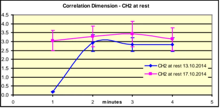
3.2. Correlation Dimension

On the basis of our previous studies on controls it results that at rest in sEMG we have usually a value of 2.7 ±

0.4 as D2 value of correlation dimension and a value of 3.80 ± 0.2 in condition of movement. In the present

in-vestigation we observed continuous transitions, exploring the condition of the subject minute by minute and

we obtained the results that are given in

Figure 13

and

Figure 14

respectively for Ch1 and Ch2. Inspection

of

Figure 13

evidences that we had a net recovery in the D2 value after the treatment with a rather stable

value, during the time transitions, remaining about 2.58 that enters in the normal range previously

indi-cated. At rest before the treatment we had rather frequent transitions oscillating from a minimum of 1.668 to

a maximum value of 3.618 both out of the normal range. In Ch2 at rest before the treatment we had continuous

transitions with values ranging from a minimum value 0.178 to a maximum value of 2.917 still entering in the

range of the normal values. After the treatment, the values of D2 stabilized about a value of 3.22 that is rather

acceptable in consideration that in Ch2 we had the left trapeze (Ch2) that was almost atrophied as we confirm

the clinical evaluation finding a value of 0.178 but still able to produce transitions arriving to 2.917 during

tran-sitions. The treatment stabilized such behaviour about the value of 3.22 that is not so distant from the normal

value. Finally we have to remember here that in any case in EMG signals we have always noise corrupted time

series and that all our results were always controlled by using surrogate data in order to dismiss the null

hy-pothesis. The conclusion is

Figure 13.

Estimation of correlation dimension in Ch1 at rest before and after

therapy.

Figure 14.

Estimation of correlation dimension in Ch2 at rest before and after

therapy.

Correlation Dimension - CH1 at rest

0.0 0.5 1.0 1.5 2.0 2.5 3.0 3.5 4.0 4.5 5.0 0 1 2 m inutes 3 4 5 CH1 at rest 13.10.2014 CH1 at rest 17.10.2014

Correlation Dimension - CH2 at rest

0.0 0.5 1.0 1.5 2.0 2.5 3.0 3.5 4.0 4.5 0 1 2 m inutes 3 4 5 CH2 at rest 13.10.2014 CH2 at rest 17.10.2014

(11)

that the analyzed data confirmed that in sEMG we are in presence of a deterministic chaotic regime that we may

delineate and quantify in detail. In particular, the results indicate that the used treatment induced unquestionable

improvement.

3.3. Estimation of the Largest Lyapunov Exponent

As previously explained, the estimation of the Largest Lyapunov Exponent represents one important step in

chaos analysis.

The Lyapunov exponent of a dynamical system is a quantity that characterizes the rate of separation of

infini-tesimally close trajectories in the attractor Quantitatively, two trajectories of the attractor reconstructed in the

phase space with initial separation

δz

0

diverge at a rate given by

δz − δz

0

exp(

λt) where λ is the Lyapunov

expo-nent that we have to estimate. It is common to refer to the largest one as the Maximal Lyapunov expoexpo-nent

λ

E

because it determines a notion of predictability for a dynamical system. A positive

λ

E

is usually taken as an

in-dication that the system is chaotic. Obviously each result must be accepted only after control using surrogate

data and evaluating the results with appropriate competence taking into account that we may have also other

cases, out of chaotic systems, in which such exponent may result positive.

Let us look at the results of our analysis. The normal value for sEMG measurement on trapeze we have

tabu-lated is

λ

E

= 0.068 ± 0.007 for health young subjects. By using surrogate data analysis we find that

λ

E

= 0.372 ±

0.008 as expected to confirm that we are actually examining a chaotic time dynamics. By these values the null

hypothesis may be dismissed and we are sure that we are examining a chaotic muscular dynamics. The previous

result relates obviously young subjects at rest for 3 minutes.

In the present case we examined right (Ch1) and left (Ch2) trapezes for a time of three minutes and we

ob-tained the following results.

At rest first control in Ch1,

λ

E

= 0.147 ± 0.004 with surrogate data result

λ

E

=0.183 ± 0.006. Therefore we

have the normal value

λ

E

= 0.068 ± 0.007 against

λ

E

= 0.147 ± 0.004 in the case of the examined muscular

dys-trophy. After the treatment we had the following estimated

λ

E

= 0.102 ± 0.006 (surrogate data value

λ

E

=0.163 ±

0.008). We verify that the treatment induced a strong improvement since

λ

E

= 0.068 ± 0.007 is our normal value.

λ

E

= 0.147 ± 0.004 before the treatment and

λ

E

= 0.102 ± 0.006 resulted after the treatment.

This is for the right trapeze. Let us examine now the results that we obtained for the left trapeze (Ch2).

At rest before the treatment we had

λ

E

= 0.101 ± 0.006 (the surrogate data analysis gave

λ

E

= 0.207 ± 0.008,

thus confirming that also in this region muscular activity followed a chaotic regime). Left Trapeze resulted less

chaotic respect to the

λ

E

value in the right trapeze with a strong unbalancing (

λ

E

= 0.147 ± 0.004 against

λ

E

=

0.101 ± 0.006) between the two (right-left) muscular dynamics. After the treatment, however, it resulted that

λ

E

= 0.115 ± 0.006 (surrogate data result

λ

E

= 0.190 ± 0.007). In conclusion, after the treatment we had

λ

E

= 0.102 ±

0.006 (Ch1) against

λ

E

= 0.115 ± 0.006 (Ch2) with a strong recovering in unbalancing situation. This was

ob-tained by the treatment lowering strongly the chaoticity in Ch1 and increasing instead lightly the value in Ch2.

This is confirmed of course from the results when we examined the attractor dimension by estimating the values

of the Correlation Dimension in Ch1 and in Ch2. Looking at the

Figure 13

and

Figure 14

in fact one verifies

that in Ch1 the value of the correlation dimension and thus the level of chaotic complexity decreases after the

treatment while instead increased that one in Ch2.

3.4. LZ Complexity

It is well known that chaotic systems posses the basic relevant property of the self-organization. Such systems

realize patterns that are self-arranged moving their time dynamics through stages on increasing complexity.

Therefore it becomes of relevant interest to evaluate the level of complexity of the system during its dynamics.

A measure of complexity in chaos analysis is reached by using the algorithmic of Lempel-Ziv that we used in

this paper. The index varies between 0 and 1. Maximal complexity (represented by pure randomness) has a

value of 1 and perfect predictability has a value of 0. Normal value in trapezes in young subjects has been

esti-mated by us to be LZ = 0.23. In Ch1 we had LZ = 0.93 (high complexity) at rest before the treatment and this

values decreased to LZ = 0.75 after the treatment. In Ch2, as well as in the case of the Correlation Dimension

and Largest Lyapunov Exponet, we estimated the opposite. We had the initial value of LZ = 0.643 at rest before

of the treatment and such value increased to LZ = 0.89 after the treatment again inducing balance between the

two regions.

(12)

E. Conte et al.

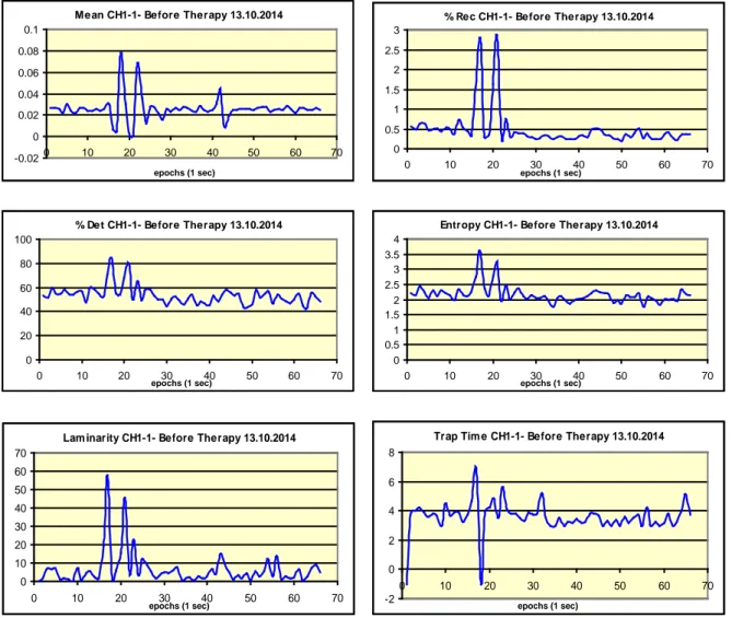
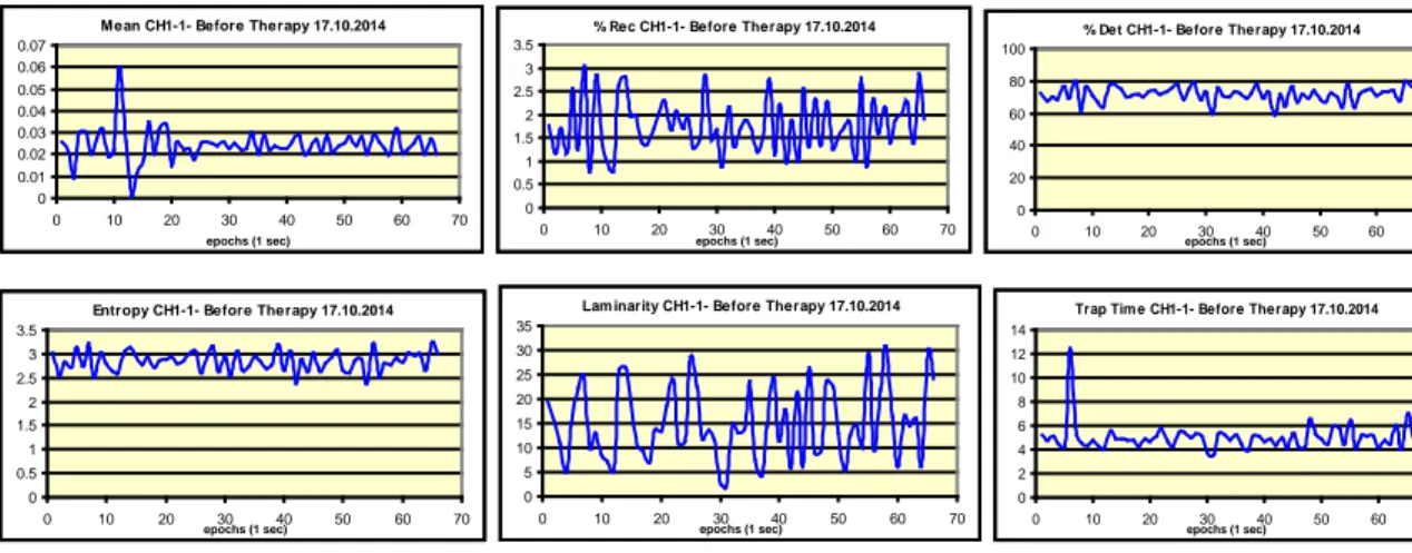
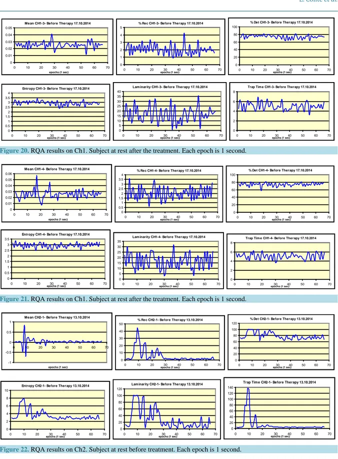
3.5. Recurrence Quantification Analysis

We may now go to examine the results that we obtained by using the previously mentioned Recurrence

Quanti-fication Analysis (RQA). In

Figures 15-17

we give the results of the analysis performed on the Ch1 subject

be-fore of the treatment while in

Figures 18-21

we have the corresponding results in Ch1 after the treatment. In

Figures 22-24

we have the results in Ch2 before the treatment. In

Figures 25-28

we have the corresponding

re-sults after the treatment. All the rere-sults are given by epochs of 1 second so that we may appreciate step by step

the dynamics and the transitions that were involved.

In

Picture 1

we have in detail the obtained results.

We repeat here that the indexes of the RQA to be estimated in each sEMG data analysis are the %Rec,

the %Det, the %Lam, the Entropy and the Trapping Time. The reason is that they are able to detect and to

quan-tify in detail the presence of repetitive hidden patterns in sEMG which, in turn, senses the level of MU

synchro-nization within the muscle in reason of the particular pathology under investigation. In the reported table we

give the results that we obtained by investigation of sEMG in epochs of 1 second., In this manner we performed

a very accurate analysis (1 second) of the muscle dynamics and its transitions of the subject affected from

mus-cular dystrophy. We performed the comparison of the obtained results for the subject at rest and before and after

the treatment. The reader may inspect the obtained values for each epoch and every time compared before

re-spect to after the treatment. It is possible to verify that we obtained an improvement of our RQA indexes in each

epoch for Ch1 (right trapeze). All the variables %Rec, %Det, %Lam, Entropy and Trapping Time increased in a

Figure 15.

RQA results on Ch1. Subject at rest before treatment. Each epoch is 1 second.

Mean CH1-1- Before Therapy 13.10.2014

-0.02 0 0.02 0.04 0.06 0.08 0.1 0 10 20 30 40 50 60 70 epochs (1 sec)

% Rec CH1-1- Before Therapy 13.10.2014

0 0.5 1 1.5 2 2.5 3 0 10 20 30 40 50 60 70 epochs (1 sec)

% Det CH1-1- Before Therapy 13.10.2014

0 20 40 60 80 100 0 10 20 30 40 50 60 70 epochs (1 sec)

Entropy CH1-1- Before Therapy 13.10.2014

0 0.5 1 1.5 2 2.5 3 3.5 4 0 10 20 30 40 50 60 70 epochs (1 sec)

Lam inarity CH1-1- Before Therapy 13.10.2014

0 10 20 30 40 50 60 70 0 10 20 30 40 50 60 70 epochs (1 sec)

Trap Tim e CH1-1- Before Therapy 13.10.2014

-2 0 2 4 6 8 0 10 20 30 40 50 60 70 epochs (1 sec)

(13)

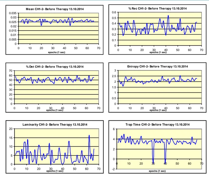
Figure 16.

RQA results on Ch1. Subject at rest before treatment. Each epoch is 1 second.

very impressive manner after the treatment respect to before the treatment. Remember that, according to the

re-sults of the RQA analysis, an increasing value in %Rec, and %Det identify the percentage of repetitive

hidden-patterns in sEMG which, in turn, senses the level of MU synchronization within the muscle. %Det in particular

characterizes chaos-order transitions, the duration of a stable interaction. Laminarity quantifies instead the level

of chaos-chaos transitions in muscle with the Trapping Time index relates the time the muscle remains in a

spe-cific state. We found such parameters all increased. Finally also Entropy resulted increased after the treatment

respect to before the treatment evidencing that the system reached a general level of relevant complexity. We

obtained instead oscillating results in Ch2 (left trapeze) before respect to after the treatment. We had epochs in

which the values of the previously mentioned variables of RQA prevailed before the treatment respect to after

the treatment and epoch in which we had the vice versa. In substance, as said, Ch1 was placed on the right

tra-pezes and Ch2 on the left Trapeze. We have to consider first of all that the tratra-pezes, are very sensitive and

reac-tive to the sympathetic nervous system so that the psychophysiological condition of the subject must be taken in

consideration as we exposed in detail in a previous papers

[9] [12] [14]

. Obviously, an increase in sympathetic

ac-tivity will contribute to tense up in the trapezes. In addition, in the dystrophic subject under consideration, clinical

inspection evidenced that there was a very significant degree of muscle tension in his right trapezes (Ch1)

com-pared to the much lesser degree of tension in his left trapezes (Ch2). So right from the very beginning, it was

always going to be the case that there would be more improvement shown in Ch1 than any other channel In

ad-dition there is also a general neurological consideration that explains the importance, previously outlined, of our

new methodology that mixes RQA analysis and time dynamics synchronization analysis devoted to the Ch1-Ch2

0 0.005 0.01 0.015 0.02 0.025 0.03 0.035 0 10 20 30 40 50 60 70 epochs (1 sec)

0 0.1 0.2 0.3 0.4 0.5 0.6 0 10 20 30 40 50 60 70 epochs (1 sec)

0 10 20 30 40 50 60 70 0 10 20 30 40 50 60 70 epochs (1 sec)

0 0.5 1 1.5 2 2.5 3 0 10 20 30 40 50 60 70 epochs (1 sec)

0 5 10 15 20 0 10 20 30 40 50 60 70 epochs (1 sec)

-2 0 2 4 6 0 10 20 30 40 50 60 70 epochs (1 sec)

(14)

E. Conte et al.

Figure 17.

RQA results on Ch1. Subject at rest before treatment. Each epoch is 1 second.

Figure 18.

RQA results on Ch1. Subject at rest after the treatment. Each epoch is 1 second.

Figure 19.

RQA results on Ch1. Subject at rest after the treatment. Each epoch is 1 second.

and Ch8 (braEEG)-Ch1 and Ch8-Ch2 and that we will publish in detail in a subsequent paper. The reason

in-volves the contra-lateral hemispheres of the brain. Ch1 is under the control of the left hemisphere of the brain

and Ch2 under the control of the right hemisphere. What these data verify is that this subject had long term right

hemisphere dominance. The subject was in a very right brain dominating state for a very long time and he had

been a very angry impatient person. The distribution of energy in the brain was not bilaterally equal, therefore

0 0.005 0.01 0.015 0.02 0.025 0.03 0.035 0 10 20 30 40 50 60 70 epochs (1 sec)

0 0.2 0.4 0.6 0.8 1 0 10 20 30 40 50 60 70 epochs (1 sec)

0 10 20 30 40 50 60 70 0 10 20 30 40 50 60 70 epochs (1 sec)

0 0.5 1 1.5 2 2.5 3 0 10 20 30 40 50 60 70 epochs (1 sec)

0 5 10 15 20 25 0 10 20 30 40 50 60 70 epochs (1 sec)

-2 0 2 4 6 0 10 20 30 40 50 60 70 epochs (1 sec)

0 0.01 0.02 0.03 0.04 0.05 0.06 0.07 0 10 20 30 40 50 60 70 epochs (1 sec)

0 0.5 1 1.5 2 2.5 3 3.5 0 10 20 30 40 50 60 70 epochs (1 sec)

0 20 40 60 80 100 0 10 20 30 40 50 60 70 epochs (1 sec)

0 0.5 1 1.5 2 2.5 3 3.5 0 10 20 30 40 50 60 70 epochs (1 sec)

0 5 10 15 20 25 30 35 0 10 20 30 40 50 60 70 epochs (1 sec)

0 2 4 6 8 10 12 14 0 10 20 30 40 50 60 70 epochs (1 sec)

0 0.01 0.02 0.03 0.04 0.05 0 10 20 30 40 50 60 70 epochs (1 sec)

0 0.5 1 1.5 2 2.5 3 3.5 4 0 10 20 30 40 50 60 70 epochs (1 sec)

0 20 40 60 80 100 0 10 20 30 40 50 60 70 epochs (1 sec)

0 0.5 1 1.5 2 2.5 3 3.5 0 10 20 30 40 50 60 70 epochs (1 sec)

0 5 10 15 20 25 30 0 10 20 30 40 50 60 70 epochs (1 sec)

0 2 4 6 8 0 10 20 30 40 50 60 70 epochs (1 sec)

(15)

Figure 20.

RQA results on Ch1. Subject at rest after the treatment. Each epoch is 1 second.

Figure 21.

RQA results on Ch1. Subject at rest after the treatment. Each epoch is 1 second.

Figure 22.

RQA results on Ch2. Subject at rest before treatment. Each epoch is 1 second.

the left hemisphere adopted a permanent hyper protective state, which was then exhibited in the excessive

mus-cle tension in his right trapezes. What the treatment enabled then, was for the distribution of energy and

infor-mation in the system to become bilaterally stable, correcting these bilateral errors seen on the contralateral sides

0 0.01 0.02 0.03 0.04 0.05 0 10 20 30 40 50 60 70 epochs (1 sec)

0 1 2 3 4 5 0 10 20 30 40 50 60 70 epochs (1 sec)

0 20 40 60 80 100 0 10 20 30 40 50 60 70 epochs (1 sec)

0 0.5 1 1.5 2 2.5 3 3.5 4 0 10 20 30 40 50 60 70 epochs (1 sec)

0 5 10 15 20 25 30 35 40 0 10 20 30 40 50 60 70 epochs (1 sec)

0 2 4 6 8 0 10 20 30 40 50 60 70 epochs (1 sec)

0 0.01 0.02 0.03 0.04 0.05 0.06 0 10 20 30 40 50 60 70 epochs (1 sec)

0 0.5 1 1.5 2 2.5 3 3.5 4 0 10 20 30 40 50 60 70 epochs (1 sec)

0 20 40 60 80 100 0 10 20 30 40 50 60 70 epochs (1 sec)

0 0.5 1 1.5 2 2.5 3 3.5 0 10 20 30 40 50 60 70 epochs (1 sec)

0 5 10 15 20 25 30 35 0 10 20 30 40 50 60 70 epochs (1 sec)

0 2 4 6 8 0 10 20 30 40 50 60 70 epochs (1 sec)

-1 -0.5 0 0.5 1 0 10 20 30 40 50 60 70 epochs (1 sec)

0 10 20 30 40 50 0 10 20 30 40 50 60 70 epochs (1 sec)

0 20 40 60 80 100 120 0 10 20 30 40 50 60 70 epochs (1 sec)

0 2 4 6 8 10 0 10 20 30 40 50 60 70 epochs (1 sec)

0 20 40 60 80 100 120 0 10 20 30 40 50 60 70 epochs (1 sec)

0 20 40 60 80 100 120 140 0 10 20 30 40 50 60 70 epochs (1 sec)

(16)

E. Conte et al.

Figure 23.

RQA results on Ch2. Subject at rest before treatment. Each epoch is 1 second.

Figure 24.

RQA results on Ch2. Subject at rest before treatment. Each epoch is 1 second.

Figure 25.

RQA results on Ch2. Subject at rest after the treatment. Each epoch is 1 second.

of the body beneath the neck. All such data will be confirmed by inspection of the results on synchronization

Ch1-Brain, Ch2-Brain that we will publish, as said, in the following paper.

Finally, returning to the RQA analysis, we have to outline that all the results were subsequently examined by

ANOVA (as reported in the next

Table 1

) and the statistical investigation confirmed that we had the most

-0.04 -0.02 0 0.02 0.04 0.06 0.08 0 10 20 30 40 50 60 70 epochs (1 sec)

0 1 2 3 4 5 0 10 20 30 40 50 60 70 epochs (1 sec)

0 20 40 60 80 100 0 10 20 30 40 50 60 70 epochs (1 sec)

0 0.5 1 1.5 2 2.5 3 3.5 4 0 10 20 30 40 50 60 70 epochs (1 sec)

0 10 20 30 40 50 60 0 10 20 30 40 50 60 70 epochs (1 sec)

0 2 4 6 8 10 0 10 20 30 40 50 60 70 epochs (1 sec)

-0.04 -0.02 0 0.02 0.04 0.06 0.08 0.1 0.12 0 10 20 30 40 50 60 70 epochs (1 sec)

0 1 2 3 4 5 0 10 20 30 40 50 60 70 epochs (1 sec)

0 20 40 60 80 100 0 10 20 30 40 50 60 70 epochs (1 sec)

0 0.5 1 1.5 2 2.5 3 3.5 4 0 10 20 30 40 50 60 70 epochs (1 sec)

0 10 20 30 40 50 0 10 20 30 40 50 60 70 epochs (1 sec)

0 2 4 6 8 10 0 10 20 30 40 50 60 70 epochs (1 sec)

0 0.01 0.02 0.03 0.04 0.05 0 10 20 30 40 50 60 70 epochs (1 sec)

0 0.2 0.4 0.6 0.8 1 1.2 0 10 20 30 40 50 60 70 epochs (1 sec)

0 10 20 30 40 50 60 70 80 0 10 20 30 40 50 60 70 epochs (1 sec)

0 0.5 1 1.5 2 2.5 3 0 10 20 30 40 50 60 70 epochs (1 sec)

0 5 10 15 20 25 0 10 20 30 40 50 60 70 epochs (1 sec)

-2 0 2 4 6 0 10 20 30 40 50 60 70 epochs (1 sec)

(17)

Figure 26.

RQA results on Ch2. Subject at rest after the treatment. Each epoch is 1 second.

Figure 27.

RQA results on Ch2. Subject at rest after the treatment. Each epoch is 1 second.

Figure 28.

RQA results on Ch2. Subject at rest after the treatment. Each epoch is 1 second.

significant level of statistical significance in the compared data before and after the treatment.

4. Conclusions

First of all let us consider that the object of the present paper was to analyze muscular dystrophy by using standard

0 0.005 0.01 0.015 0.02 0.025 0.03 0.035 0.04 0 10 20 30 40 50 60 70 epochs (1 sec)

0 0.1 0.2 0.3 0.4 0.5 0.6 0.7 0.8 0 10 20 30 40 50 60 70 epochs (1 sec)

0 10 20 30 40 50 60 70 80 0 10 20 _{epochs (1 sec)}30 40 50 60 70

0 0.5 1 1.5 2 2.5 3 0 10 20 30 40 50 60 70 epochs (1 sec)

0 5 10 15 20 25 30 35 0 10 20 30 40 50 60 70 epochs (1 sec)

-2 0 2 4 6 8 0 10 20 30 40 50 60 70 epochs (1 sec)

0 0.005 0.01 0.015 0.02 0.025 0.03 0.035 0.04 0 10 20 30 40 50 60 70 epochs (1 sec)

0 0.2 0.4 0.6 0.8 1 1.2 1.4 0 10 20 30 40 50 60 70 epochs (1 sec)

0 10 20 30 40 50 60 70 0 10 20 30 40 50 60 70 epochs (1 sec)

0 0.5 1 1.5 2 2.5 3 0 10 20 30 40 50 60 70 epochs (1 sec)

0 5 10 15 20 25 30 0 10 20 30 40 50 60 70 epochs (1 sec)

-2 0 2 4 6 8 0 10 20 30 40 50 60 70 epochs (1 sec)

0 0.02 0.04 0.06 0.08 0.1 0 10 20 30 40 50 60 70 epochs (1 sec)

-5 0 5 10 15 20 0 10 20 30 40 50 60 70 epochs (1 sec)

0 20 40 60 80 100 0 10 20 30 40 50 60 70 epochs (1 sec)

0 1 2 3 4 5 0 10 20 30 40 50 60 70 epochs (1 sec)

0 10 20 30 40 50 60 70 80 0 10 20 30 40 50 60 70 epochs (1 sec)

-2 0 2 4 6 8 10 12 0 10 20 30 40 50 60 70 epochs (1 sec)

(18)

E. Conte et al.

Mean in Epochs St dev in Epochs Mean b t CH1-1-13.10 0.02562 0.00141 0.027 0.027 0.026 0.022 0.03 0.024 0.022 0.027 0.027 0.024 0.024 0.026 0.024 0.026 0.03 0.007 0.005 0.078 0.03 0 Mean b t CH1-1-17.10 0.02430 0.00424 0.026 0.021 0.009 0.03 0.03 0.02 0.027 0.032 0.019 0.022 0.06 0.026 0.001 0.011 0.018 0.035 0.02 0.032 0.034 0.015 %Rec b t CH1-1-13.10 0.48665 0.12869 0.556 0.478 0.638 0.646 0.461 0.479 0.512 0.44 0.536 0.484 0.377 0.736 0.544 0.437 0.337 1.538 2.784 0.289 0.374 1.623 %Rec b t CH1-1-17.10 1.77220 0.08839 1.771 1.174 1.706 1.186 2.552 1.266 3.04 0.763 2.859 1.485 0.997 0.797 2.627 2.815 1.965 1.999 1.405 1.376 1.695 2.056 %Det b t CH1-1-13.10 53.54055 3.71019 53.4 51.97 59.61 54.48 55.12 58.16 54.27 54.38 56.83 56.77 47.81 60.05 57.75 54.5 52.68 71.25 84.66 54.62 53.83 67.57 %Det b t CH1-1-17.10 71.65464 2.64034 72.5 67.94 70.01 68.87 76.75 68.97 79.54 61.37 76.27 70.71 66.62 63.99 77.41 78.01 75.09 70.07 71.01 71.52 70.49 73.21 Entropy b t CH1-1-13.10 2.16532 0.05798 2.212 2.149 2.432 2.238 2.059 2.298 2.113 2.31 2.205 2.13 1.992 2.326 2.153 2.117 2.248 2.761 3.608 2.362 2.121 2.785 Entropy b t CH1-1-17.10 2.84888 0.01980 3.034 2.556 2.84 2.726 3.135 2.733 3.216 2.526 3.021 2.803 2.638 2.599 3.052 3.134 2.97 2.767 2.951 2.704 2.863 2.879 Laminarity b t CH1-1-13.10 6.41933 3.45634 0 1.76 6.739 6.662 7.292 1.291 1.642 1.235 0.277 6.949 0.72 4.565 5.503 2.377 1.908 19.68 57.62 0 6.011 15.64 Laminarity b t CH1-1-17.10 14.93989 3.22370 19.55 15.35 11.14 5.001 14.87 22.36 24.63 9.981 13.18 8.337 7.187 5.366 26.15 26.32 19.21 10.34 9.433 6.932 13.53 13.29 Trap Time b t CH1-1-13.10 3.56989 3.32340 -1 3.778 4.047 4.244 3.886 3.571 3.778 3.667 3 4.533 3.667 3.886 3.903 3.231 3.714 4.672 6.839 -1 3.957 4.244 Trap Time b t CH1-1-17.10 4.99612 0.10465 5.228 4.828 5.059 4.444 4.252 12.45 5.187 4.597 4.33 4.771 4.265 4.119 5.558 4.923 4.879 4.777 4.743 4.196 4.936 4.682 Mean b t CH1-2-13.10 0.02586 0.00000 0.025 0.025 0.027 0.027 0.023 0.027 0.028 0.023 0.027 0.027 0.026 0.026 0.025 0.025 0.025 0.026 0.026 0.027 0.028 0.021 Mean b t CH1-2-17.10 0.02488 0.00283 0.029 0.02 0.028 0.02 0.029 0.022 0.025 0.024 0.027 0.017 0.033 0.018 0.031 0.02 0.027 0.042 0.035 0.014 0.021 0.018 %Rec b t CH1-2-13.10 0.31773 0.01061 0.403 0.33 0.353 0.185 0.222 0.407 0.279 0.438 0.361 0.327 0.277 0.245 0.455 0.348 0.186 0.245 0.298 0.287 0.207 0.296 %Rec b t CH1-2-17.10 1.89530 0.26941 2.174 1.085 2.415 1.385 2.914 1.537 2.278 1.605 2.169 1.698 2.01 1.405 2.036 0.786 2.342 1.143 2.109 1.891 1.91 1.656 %Det b t CH1-2-13.10 50.65402 2.21819 58.34 47.83 50.88 44.25 47.05 53.52 52.3 56.67 53.9 48.9 53.03 50.71 53.64 55.26 42.9 50 49.59 47.68 44.5 54.35 %Det b t CH1-2-17.10 73.08662 1.59382 76.04 67.12 75.24 72.08 77.33 70.55 76.57 68.64 75.4 71.48 70.32 70.21 71.85 63.28 76.22 67.21 75.64 74.55 70.83 69.31 Entropy b t CH1-2-13.10 2.08277 0.10394 2.145 1.807 1.949 1.582 1.883 2.396 2.305 2.03 2.206 2.146 2.383 2.062 2.214 2.198 1.909 1.947 2.066 1.958 1.932 2.046 Entropy b t CH1-2-17.10 2.89212 0.06505 2.96 2.65 3.093 2.787 3.087 2.725 3.034 2.562 2.954 2.775 2.824 2.729 2.848 2.472 3.016 2.72 3.006 2.875 2.739 2.816 Laminarity b t CH1-2-13.10 4.90455 2.29103 5.399 7.335 6.797 7.353 1.78 8.384 2.92 12.37 12.31 3.25 13.99 0.303 7.011 5.611 1.195 2.923 8.056 0.516 4.665 10.7 Laminarity b t CH1-2-17.10 13.28547 4.99217 19.81 6.404 19.03 13.25 26.79 25.83 16.45 12.12 8.728 8.882 11.28 8.341 13.4 4.972 17.65 14.96 17.32 18.33 7.661 18.06 Trap Time b t CH1-2-13.10 3.40208 0.41224 3.259 4.083 3.345 4.583 4 4.929 3.3 3.712 4.39 3.308 4.486 3 3.909 3.435 3 3.222 3.731 3 3.545 4.571 Trap Time b t CH1-2-17.10 4.83695 0.61377 5.444 4.194 5.311 6.509 5.408 5.389 5.764 4.523 4.453 4.88 4.826 4.647 4.329 4.051 5.429 4.494 5.093 4.658 4.29 4.879 Mean b t CH1-3-13.10 0.02619 #DIV/0! 0.026 0.026 0.026 0.026 0.027 0.026 0.024 0.028 0.026 0.026 0.026 0.027 0.025 0.027 0.027 0.025 0.027 0.024 0.028 0.027 Mean b t CH1-3-17.10 0.02532 0.00141 0.028 0.024 0.028 0.024 0.027 0.022 0.025 0.022 0.029 0.019 0.031 0.021 0.025 0.027 0.024 0.029 0.023 0.025 0.025 0.027 %Rec b t CH1-3-13.10 0.36329 #DIV/0! 0.367 0.469 0.354 0.175 0.362 0.287 0.353 0.382 0.38 0.238 0.272 0.245 0.331 0.6 0.345 0.379 0.3 0.26 0.346 0.293 %Rec b t CH1-3-17.10 2.02494 0.16051 1.83 2.578 2.844 1.274 2.74 1.355 2.46 1.771 2.466 2.052 2.664 1.662 3.17 1.846 2.54 1.575 2.592 1.831 3.338 2.201 %Det b t CH1-3-13.10 51.72107 #DIV/0! 53.95 52.29 53.28 43.87 52.77 50.99 53.15 50.13 53.74 49.79 50.86 40.02 51.72 61.04 52.12 53.16 44.44 45.67 50.04 51.01 %Det b t CH1-3-17.10 73.97953 1.17663 71.73 78.75 80.49 67.64 77.19 69.78 75.95 77.47 77.55 78.69 77.94 73.62 77.97 74.33 77.97 76.13 77.31 75.61 81.63 76.11 Entropy b t CH1-3-13.10 2.12652 #DIV/0! 2.208 2.147 2.199 1.913 2.2 2.198 2.056 1.927 2.056 2.064 2.047 1.732 2.129 2.316 2.074 2.149 2.066 1.687 2.042 2.22 Entropy b t CH1-3-17.10 2.93038 0.07071 2.78 3.265 3.094 2.725 3.175 2.685 2.939 3.065 3.106 2.954 3.171 2.831 3.165 2.972 3.089 3.18 3.104 2.941 3.379 2.94 Laminarity b t CH1-3-13.10 5.80805 #DIV/0! 11.26 12.28 1.606 0.846 2.256 5.503 2.937 3.174 6.043 2.599 6.267 0.605 5.522 4.448 3.369 1.759 0.494 2.474 3.36 1.518 Laminarity b t CH1-3-17.10 16.46862 4.19244 13.74 27.57 19.33 10.09 22.28 7.792 13.43 31.53 17.23 25.49 11.26 15.1 9.793 8.692 18.75 20.63 15.34 22.52 30.91 7.963 Trap Time b t CH1-3-13.10 3.56883 #DIV/0! 4.282 3.949 3.833 3 3.3 3.556 3.231 3.267 3.577 3.125 3.45 3 3.524 4.154 3.133 3.375 3 3.714 3.357 4.5 Trap Time b t CH1-3-17.10 5.00985 0.94894 4.48 6.198 5.602 4 5.538 3.882 4.967 6.172 5.257 5.845 5.514 5.286 4.502 3.91 5.016 6.885 4.36 6.201 6.193 4.051 Mean in Epochs St dev in Epochs Mean b t CH2-1-13.10 0.02294 0.02616 0.014 0.023 -0.01 0.033 0.018 -0.08 -0.43 0.836 -0.7 0.168 0.233 0.071 0.079 0.092 0.191 0.023 -0.05 -0.06 -0.01 -0.08 Mean b t CH2-1-17.10 0.02177 0.00283 0.022 0.018 0.002 0.023 0.039 0.004 0.034 0.036 0.025 0.015 0.029 0.028 0.013 0.018 0.013 0.023 0.025 0.013 0.024 0.027 %Rec b t CH2-1-13.10 5.57521 0.22698 1.296 1.846 1.469 0.996 1.945 7.436 24.11 24.58 43.74 36.48 21.53 2.849 7.92 21.43 23.55 0.813 1.681 4.166 2.335 13.38 %Rec b t CH2-1-17.10 0.42677 0.37335 0.792 0.928 0.696 0.62 0.957 0.697 0.844 0.497 0.829 0.533 0.595 0.295 0.443 0.471 0.488 0.418 0.301 0.317 0.174 0.232 %Det b t CH2-1-13.10 78.49726 3.66423 72.77 69.5 72.43 71.97 76.61 90.65 99.52 99.22 99.69 99.67 97.55 80.26 88.87 98.23 98.63 64.96 77.37 84.02 74.85 93.46 %Det b t CH2-1-17.10 54.01748 13.20522 61.57 69.6 64.35 58.33 66.87 64.14 68.95 56.97 63.73 56.94 56.11 45.55 58.84 55.64 56.51 50.41 49.06 47.7 47.23 45.75 Entropy b t CH2-1-13.10 3.52705 0.15910 2.853 2.759 2.827 2.782 3.074 4.248 6.845 7.141 7.587 7.856 5.935 3.376 3.899 6.096 6.483 2.627 3.066 3.526 3.029 4.539 Entropy b t CH2-1-17.10 2.17786 0.40093 2.472 2.617 2.681 2.313 2.596 2.54 2.683 2.177 2.57 2.299 2.381 1.747 2.411 2.326 2.278 1.956 2.122 1.802 1.792 1.83 Laminarity b t CH2-1-13.10 28.70786 2.04566 12.41 8.532 6.864 9.353 30.69 59.73 99.64 99.28 99.76 99.64 91.3 30.57 45.56 95.37 97.61 6.113 24.31 33.77 27.53 71.31 Laminarity b t CH2-1-17.10 6.56533 11.40422 17.9 17.29 10.65 0.957 2.97 11.85 9.402 0 16.82 9.559 16.36 2.768 16.4 4.038 14.65 13.73 8.45 3.429 0.569 2.447 Trap Time b t CH2-1-13.10 12.75483 0.46669 4.459 3.747 4.163 4.384 5.963 8.523 78.82 77.69 136.6 131.9 23.98 5.881 6.453 30.24 45.99 3.655 5.215 5.884 6.12 10.61 Trap Time b t CH2-1-17.10 3.59038 1.25370 5.573 4.636 4.412 3 3.966 3.976 5.441 -1 4.78 4.12 3.788 3.3 4.82 3.5 3.705 3.515 3.219 3.385 4 3.286 Mean b t CH2-2-13.10 0.02235 0.02758 0.004 0.053 0.006 -0 0.067 0.001 0.018 0.045 -0.01 0.051 0.021 -0 0.049 0.005 0.032 0.017 0.005 0.009 0.04 0.042 Mean b t CH2-2-17.10 0.02164 0.00141 0.019 0.019 0.021 0.023 0.021 0.035 0.016 0.019 0.015 0.026 0.025 0.021 0.019 0.02 0.019 0.019 0.032 0.016 0.027 0.015 %Rec b t CH2-2-13.10 1.90232 0.48861 1.873 0.846 2.851 2.666 0.602 2.689 3.067 1.342 2.172 2.175 1.74 1.713 1.004 2.609 1.699 2.12 1.388 2.548 2.522 1.582 %Rec b t CH2-2-17.10 0.38409 0.04101 0.25 0.278 0.284 0.214 0.398 0.373 0.396 0.297 0.376 0.31 0.344 0.386 0.409 0.372 0.355 0.354 0.514 0.458 0.439 0.44 %Det b t CH2-2-13.10 75.55823 2.65377 74.49 64.69 81.57 82.16 60.03 81.52 83.83 73.6 80.49 78.91 73.48 71.55 66.8 76.59 74.7 77.07 70.21 80.41 79.03 73.29 %Det b t CH2-2-17.10 52.49403 0.02899 47.63 50.85 47.65 41.55 48.85 51.99 51.47 47.34 51.91 58.04 47.84 54.94 58.71 58.5 55.46 53.25 51.66 55.45 49.78 57.31 Entropy b t CH2-2-13.10 3.04792 0.00849 2.898 2.425 3.374 3.367 2.393 3.258 3.577 3.048 3.194 3.268 2.808 2.813 2.617 3.273 2.968 3.047 2.769 3.295 3.141 2.99 Entropy b t CH2-2-17.10 2.15964 0.22486 1.918 1.983 1.83 1.855 2.268 2.113 2.152 2.115 2.099 2.067 1.829 2.259 2.371 2.274 2.053 2.193 2.127 2.211 2.219 2.389 Laminarity b t CH2-2-13.10 18.20074 9.70151 20.14 3.157 27.32 23.51 2.872 28.88 34.39 15.38 21.28 21.03 9.348 15.18 9.901 28.6 15.12 18.79 15.49 22.12 17 11.97 Laminarity b t CH2-2-17.10 7.17179 1.89010 3.557 0.801 4.435 1.852 3.605 8.94 9.295 5.824 16.58 4.936 3.669 6.282 12.15 4.183 4.593 6.001 7.593 19.76 8.512 13.27 Trap Time b t CH2-2-13.10 5.25252 0.21708 5.104 3.484 5.478 5.937 3.5 7.125 6.061 5.799 5.109 5.127 4.273 4.191 3.903 7.842 5.093 6.172 4.78 5.217 5.176 4.699 Trap Time b t CH2-2-17.10 3.60242 0.27860 3.273 3 3.188 3.2 3.222 3.553 3.239 3.5 3.877 3.647 3.4 3.5 3.941 4.2 3.3 4.095 3.435 4.357 3.432 4.37 Mean b t CH2-3-13.10 0.02262 #DIV/0! 0.03 0.037 -0.01 0.057 0.01 0.002 0.059 0.01 0.001 0.059 -0.01 0.014 0.053 -0.01 0.047 0.023 0.001 0.052 -0.01 0.044 Mean b t CH2-3-17.10 0.02177 0.00141 0.019 0.024 0.022 0.018 0.021 0.016 0.023 0.025 0.024 0.02 0.019 0.022 0.022 0.022 0.023 0.023 0.015 0.018 0.029 0.022 %Rec b t CH2-3-13.10 2.02916 #DIV/0! 2.595 0.992 1.319 0.721 2.132 2.466 0.76 2.987 1.858 1.034 1.695 3.622 0.953 1.942 2.439 2.109 1.954 1.406 2.324 2.142 %Rec b t CH2-3-17.10 0.41117 0.20577 0.557 0.272 0.557 0.371 0.427 0.284 0.444 0.513 0.387 0.642 0.395 0.344 0.408 0.243 0.489 0.368 0.482 0.332 0.288 0.377 %Det b t CH2-3-13.10 76.89857 #DIV/0! 82.5 67.45 75.58 64.48 80.69 80.71 64.57 83.92 79.27 73.32 78.26 82.34 65.21 79.49 79.42 77.61 76.87 74.15 75.9 78.49 %Det b t CH2-3-17.10 54.47258 6.27628 57.25 49.86 58.52 53.4 58.59 52.13 55.57 56.41 54.6 59.55 51.56 52.45 52.4 44.41 56.54 54.64 58.89 51.71 48.67 50.2 Entropy b t CH2-3-13.10 3.10533 #DIV/0! 3.449 2.517 3.109 2.479 3.289 3.276 2.635 3.592 3.119 2.871 3.114 3.537 2.535 3.195 3.394 3.098 3.038 2.845 3.033 3.135 Entropy b t CH2-3-17.10 2.19841 0.24678 2.299 2.231 2.351 1.989 2.049 2.133 2.258 2.326 2.171 2.546 2.007 2.22 2.053 2.075 2.326 2.026 2.348 2.141 2.037 2.125 Laminarity b t CH2-3-13.10 18.42203 #DIV/0! 25.86 4.511 9.953 5.039 27.19 20.15 3.741 33.56 6.386 18.46 11.59 25.64 9.282 25.14 18.45 12.42 7.174 9.022 11.15 14.37 Laminarity b t CH2-3-17.10 7.68644 0.16122 6.829 8.917 10.65 9.133 6.189 5.918 9.577 11.43 7.344 12.56 9.512 0.647 6.125 8.943 17.23 2.083 6.612 2.455 0 9.174 Trap Time b t CH2-3-13.10 5.38860 #DIV/0! 5.496 3.935 4.827 4.594 5.651 5.334 3.71 5.851 3.871 5.805 4.76 5.648 4.068 6.54 5.233 5.067 4.109 5.13 4.721 4.882 Trap Time b t CH2-3-17.10 3.76294 0.03536 3.85 4.083 4.068 3.605 3.821 3.778 4.195 3.885 3.71 3.747 3.8 3 3.741 4.632 5.09 3.1 4.448 3.3 -1 3.415