A MULTISCALE FEATURE EXTRACTION APPROACH FOR 3D RANGE IMAGES
F. Bonarrigo
∗, A. Signoroni, R. Leonardi
University of Brescia
Dept. of Information Engineering
via Branze 38, I25123, Brescia, Italy
M. Carocci
Open Technologies srl
via IV Novembre 14
I25010, S. Zeno Naviglio, Brescia, Italy
ABSTRACT
This paper presents a multiscale feature extraction technique for 3D range images. Optimized and improved 3D Gaussian filtering and saliency map computation have been conceived jointly to the exploitation of connectivity relationships natu-rally induced by the 2D acquisition grid. The proposed al-gorithmic and implementation solutions guarantee good re-peatability of detected features on different views and demon-strated superior computational performance compared to other known approaches.
1. INTRODUCTION
Nowadays, there is a growing interest in 3D shape acquisi-tion and analysis because of their broad range of applicaacquisi-tion fields (industrial, entertainment, security, medical, cultural heritage,...). In order to acquire the 3D shape of an object, a stereo scan system is usually employed to obtain a set of 3D range images (RI). If no information about relative displace-ments between scanner and object is available, the different views will not share a common reference system. In order to reconstruct the object shape, it is thus necessary to accurately align each view of the acquisition dataset through a registra-tion procedure. A way to estimate the relative displacement between two views consists into the identification of a set of corresponding points taken from each view and the computa-tion of an optimal rototranslacomputa-tion matrix out of them. Brute force approaches to solve this problem become impractical as RI size increases. In order to speed-up this procedure, a com-mon technique is to reduce the number of candidates by au-tomatically extracting a small set of feature points from both views and searching for correspondences between them. The problem then becomes how to select feature points that, with high repeatability rate, appear in same positions on overlap-ping areas of different views, i.e. taken from different angle directions. Feature extraction repeatability performance are important within a feature based model acquisition pipeline in that it heavily influences subsequent steps toward automated view alignment for 3D model acquisition [1]. Different so-lutions have been proposed for 3D feature extraction. In [2]
∗The first author performed the work while at Open Technologies srl, Italy
points are selected based on curvature criteria. In [3], for each point of the RI, the volume portion of the object inscribed into a sphere surrounding the point is estimated and only un-common values are selected. Other solutions, like the pre-sented one, are based on multiscale analyses [4], [5], [6] and are somewhat inspired to the Lowe’s SIFT approach [7]. Al-though differing in algorithmic and implementation aspects, a typical sequence of processing steps for feature point extrac-tion is:
• calculate the normals to the RI points (preliminary step) • calculate N Gaussian filtered (scaled) versions of the RI • derive N-1 saliency maps from the filtered data • identify local maxima on each saliency map
Following this approach, we present some improving solu-tions for feature detection on 3D range data and we measure their performance in terms of feature repeatability and com-putation speed. Our main contributions are 1) a new direction-constrained Gaussian-like filtering, and 2) naturally induced neighborhood exploitation for computational speed-up. 2. FEATURE EXTRACTION ON 3D RANGE IMAGES In a RI, each acquired pixel (usually on a image sensing grid x = (w, h)) is associated to a depth or distance information (according to the modeled acquisition geometry). Some scan-ners produce true 3D localization of the point in the acqui-sition coordinate system. In our formalism a range image is a map RI : I(Z2
) → R(R3), where the domain I is a
regular rectangular grid (usually corresponding to the CCD matrix), and the co-domain R corresponds to the set of 3D points belonging to the target object. Not all points in I have a valid corresponding point px ∈ R (this is due to the na-ture of the acquisition in terms of target object shape and/or measure range limitations) so a valid point subset Iv ⊆ I
can be defined. Moreover, although the 2D index grid is uni-formly distributed, 3D points cannot be considered uniuni-formly distributed over the 3D space. This is because point density is inversely proportional to the angle existing between the ac-quisition direction, and the normal associated to each point. Considering R as a surface, its point distribution presents
holes in correspondence to occlusions, i.e. parts of the tar-get object that are not directly visible by the incident rays. Despite these facts (non-valid regions, non-uniform density and holes) the regularity of the 2D grid is a useful structuring resource that can be used as a naturally induced connectivity lattice to be exploited in 3D point processing and to determine practical definitions to various data processing operators (e.g. filtering, interpolation/subsampling, normal computation,...) and speed-up their computation. We exploit this connectiv-ity in all the steps of our method, and we propose original implementations of Gaussian filtering and saliency map cal-culations on RIs.
2.1. Normal extraction
Our feature extraction algorithm requires the computation of normal vectors at each point location px ∈ R. Given a px, its normal is computed by calculating the difference vectors d = pj− px between px and its 8 neighbor points pj in the 2D index grid. By assigning an index k, ranging from 1 to 8, for each vector d, associated in a anti-clockwise order (see Fig.1), we define the normal ˆnxas:
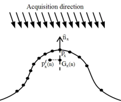
ˆ nx= 8 X k=1 ˆ dk× ˆdj 8 j = ( k + 2 k <= 6 k − 6 k > 6 (1) (a) (b) · · · (c) Fig. 1. ˆd selection for (a) k = 1; (b) k = 2; (c) k = 8
2.2. 3D Gaussian filtering
An important step for our algorithm requires to extract a set of N Gaussian filtered versions G (n) of the input range image, with n = [1, N ]. In order to do so, N 3D Gaussian filters with progressively increasing kernel dimension σn are applied to
each point constituting the original range image, varying its position as follows: pfx (n) = X pj∈ηx(2σn) pj· e− kpx−pjk2 2·σ2n X pj∈ηx(2σn) e− kpx−pjk2 2·σ2n (2)
where σn represents the nth kernel radius, while ηx(2σn)
identifies the points within a distance 2σnfrom px.
Fig. 2. pfx (n) projected over ˆnxdirection
The set of pfx (n), as calculated in (2), could be directly used
(as done in [5] and [6]) as filtered data. However, we do not yet consider it as such. This is because, due to the above de-scribed characteristics of R, border points (on validity region or hole boundaries) and points lying between two regions with different normal directions would suffer from shrinking and position biasing distortions respectively. These distortions cannot be considered negligible, since most feature points are located over highest curvature regions and therefore they are prone to position biasing due to point density disparity over ηx(2σn). In addition, shrinking distortion would affect
bor-der areas and would lead to artifacts in the saliency compu-tation, as we will see. In order to avoid such distortions, we propose to project pfx(n) over the normal direction ˆnx, as
fol-lows:
Gx(n) = px+p f
x(n) − px, ˆnx ˆnx (3)
This is equivalent to force pfx(n) to move along the axis
associated to ˆnx, therefore reducing the distortion caused by
non-uniform points distribution over ηx(2σn), as depicted in
Fig.2.
We define G (n), the set of points Gx(n) , ∀x ∈ RI, as the
fil-tered version of the range image after having applied a Gaus-sian filter of radius σn, as defined in (3). As the kernel radius
σn increases, details which size is smaller than σndisappear
from G (n). Once the G (n) has been calculated, its normal vectors are recomputed as indicated in section 2.1.
As usually done in multiscale approaches, when kernel size doubles, a subsampling factor of two is applied to the image, also to reduce the computational burden. Here subsampling is performed on I, thus in a very simple and fast way. 2.3. Saliency maps calculation
Once the G (n) have been computed, N-1 saliency maps can be derived. A saliency map is a 2D array of difference values, obtained by pairwise subtraction of G (n) at different kernel sizes. In a multiscale framework, a pairwise subtraction be-tween G (n) retains only the details comprised bebe-tween the two scale limits (which can be roughly thought as cut-off frequencies), in other words it highlights features which di-mension is comprised between two kernel sizes, say σn and
σn+1. Thanks to the shrinking artifact avoidance
guaran-teed by (3), straightforward pointwise subtraction at different scales can be performed correctly. We then calculate saliency maps S (n) as follows:
S (n) = |G (n) − G (n + 1)| · hˆnx(n) , ˆnx(n + 1)i (4)
Unlike [4] and [5], the factor hˆnx(n) , ˆnx(n + 1)i has been
in-troduced in order to give more importance to points for which the normal direction does not change after the filtering pro-cess, thus restricting saliency distribution to more specific ar-eas of the range image. A similar approach is employed in [6], where the correction factor takes into account ˆnx(n).
2.4. Maximum extraction
Once each saliency map S (n) has been determined, saliency maximums are extracted as follows:
sM ax (n) = {x | Sx(n) > Sj(n) , ∀j ∈ ηx(2σn+1)} (5)
In order to generate the maximum list for a saliency map, an iterative search is performed. Once the greatest valid saliency value for S (n) is found, no other maximum may be selected within a neighborhood region of ηx(2σn+1). This is because
the greatest detail size that can be detected within S (n) is σn+1. Such constraints on the distance between maxima
guar-antee the absence of overlap between features.
Each maximum is further tested through two conditions be-fore being selected as feature point. At first, its neighbor-hood must be defined. In order to avoid selecting features which descriptor would result calculated out of few neigh-bor points, maximums that possess less than 50% of the es-timated points for ηx(2σn) are discarded. The second check
is about position stability. Saliency maps may slightly vary due to changes of acquisition direction, therefore maximums detected over regions with similar saliency values may vary their position significantly. In order to avoid such points, we only retain maximums for which the saliency value is much greater than its neighboring points, and it is not located over saliency ridges. An example of saliency map with superim-posed feature points at a given scale is shown in Fig.3.
3. RESULTS
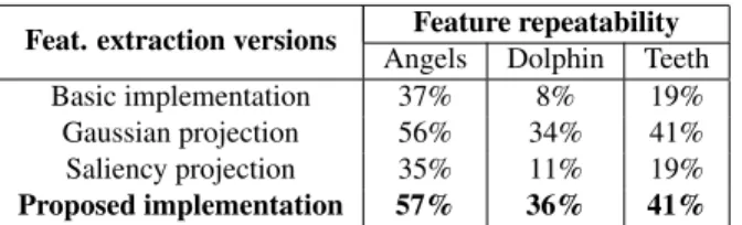
To assess the contribution of each step and the overall per-formance of the proposed feature extraction method, four dif-ferent implementations have been tested, depending on which version of filtering and saliency computation have been used. The first version, we called basic implementation, reflects what proposed in [5], i.e. Gaussian filtering performed as in (2) and saliency computed as pairwise difference between fil-tered versions of data. The second version only implements the improved version of Gaussian filter (3); the third ver-sion only implements the saliency correction (4). Al last, the
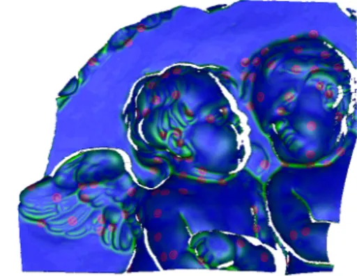
Fig. 3. A saliency map with superimposed feature points.
Fig. 4. Datasets: (a) Angels, (b) Dolphin, (c) Teeth.
fourth version implements both the proposed improvements. The comparison has been performed over three pre-aligned range image datasets which are shown in Fig.4 (where differ-ent colors have been used for each view). All RIs have been acquired with a commercial structured-light scanner (Optical Rev-Eng LE, produced by Open Technologies srl, Italy). All the range images used for our tests have a resolution of 1280 × 1024, which means that Iv can have up to over 1.3
mil-lion points. Prior to the first Gaussian filtering, each range image is down-sampled by a factor 2, thus reducing initial di-mensions to 640×512. In our implementation, three G (n) have been calculated, with σn = 2σn−1, while the σ1is set
to be eight times the average interdistance between points in R. Although, according to the SIFT methodology [7], the implemented software can work with any number of scaling level and σ progression, we experimentally found the above parameters to give the best compromise between repeatability and computational performances for the considered datasets. Repeatability performance evaluations have been executed as follows: from each range image of a dataset, its features are extracted, then for each pair of consecutive range images (ac-cording to a predetermined order), features in the overlapping area are counted; subsequently, both feature sets are com-pared in order to find correspondences (feature points are con-sidered correspondent if their position differ in less than σ3). At last, feature repeatability is computed as the number of features that have a correspondence relation divided by the
Feat. extraction versions Feature repeatability Angels Dolphin Teeth
Basic implementation 37% 8% 19%
Gaussian projection 56% 34% 41%
Saliency projection 35% 11% 19%
Proposed implementation 57% 36% 41%
Table 1. Repeatability performance
Dataset RI Min-max Avg points Exec time
name No. overlap (×103) [ms]
Angels 8 20-60% 1040 4823
Dolphin 20 20-90% 406 1894
Teeth 8 40-90% 408 1836
Table 2. Computational performance
number of features in the overlapping area. In Table1, feature repeatability performances are presented for each dataset and for each feature extraction version. Reported data are aver-aged over all scales and all couples of overlapping RIs. Our evaluation shows that the modified Gaussian filter improves repeatability performances by more than 20 percentage points with respect to the basic implementation of the Gaussian fil-ter (used in the first and third version). Such improvement is due to the fact that the proposed filter does not introduce any shrinking effect usually associated to the Gaussian filter-ing, thus improving feature localization. The saliency correc-tion does not yield as much, however a slight performance improvement is achieved through its introduction. It can be argued that such repeatability rates may not be considered as extraordinary. As a matter of fact, to our knowledge, no study about feature repeatability have been published. In [4], some feature repeatability results against range data subsampling and noise addition are presented, but they are not useful here for comparison. We deem our performances to be satisfactory because of two reasons. The first one is related to the image sets employed, since they present a heterogeneous grade of regularity, different feature types and dimensions, and usually big differences (borders, holes, point density) when acquired with different acquisition directions. Secondly, we deem such repeatability rates as entirely adequate for a robust subsequent search of correspondences, if suitable feature descriptors or signatures can be calculated and used to this end.
Computational performances are presented in Table 2, where we also describe datasets in terms of number of RI views per dataset, min-max overlap area between views pairs, and av-erage number of points (i.e. |Iv|) per RI. Algorithms have
been implemented in C++, and executed on a PC with INTEL CORE2 CPU, 2.80 GHz each, and 4 GB of RAM. As the differences in computational time for the above four versions are negligible, we only give the processing time required by the proposed implementation, which is around 4.5 seconds for each million of points. This is quite an improvement with respect to [5] (around 5 minutes per million points), [4] (50
minutes per million points), [3] (around 5 minutes per million points) and [6] (around 7 minutes per million points), even considering the upgraded computational resources. Such per-formance boost is mainly due to the exploitation of neigh-borhood relationships defined on I. Secondly, the use of a fast subsampling, and some coding efficiency solutions on frequent and time-consuming operations make the rest (e.g. look-up tables for square root computing).
4. CONCLUSION
In this paper a multiscale method for 3D feature extraction on range images has been presented. This method, that can also be considered as a 3D extension of a SIFT-based approach, demonstrated to yield good robustness in terms of feature re-peatability, and outstanding computational performance. The work is mainly characterized by the introduction of a modi-fied version of Gaussian filtering of 3D range images and a weighted saliency map computation. They both contribute to improve feature repeatability. In addition, the direct ex-ploitation of the 2D domain neighborhood helps the definition of the filter action and is determinant for the computational speed. Experimental performance confirm that our method is suitable to be used for automated multiple view registration and 3D model acquisition, where the degree of accuracy and obtainable automation strongly depends from the goodness of the feature extraction phases. The proposed solutions can be also useful for other 3D feature-based applications, such as content analysis and description of 3D objects, 3D object tracking, etc., where features robustness and computational speed are crucial aspects.
5. REFERENCES
[1] F. Bernardini and H. Rushmeier, “The 3D model acquisition pipeline,” Computer Graphics Forum, vol. 21, no. 2, pp. 149– 172, 2002.
[2] S. M. Yamany and A. A. Farag, “Surfacing signatures: An orien-tation independent free-form surface represenorien-tation scheme for the purpose of objects registration and matching,” IEEE Trans. on Pattern Analysis and Machine Intelligence, vol. 24, no. 8, pp. 1105–1120, 2002.
[3] N. Gelfand, N. J. Mitra, L. J. Guibas, and H. Pottmann, “Robust global registration,” in Symp. Geom. Processing, 2005. [4] X. Li and I. Guskov, “Multi-scale features for approximate
alignment of point-based surfaces,” in Symp. Geom. Process-ing, 2005.
[5] C. H. Lee, A. Varshney, and D. W. Jacobs, “Mesh saliency,” in SIGGRAPH ’05, 2005, pp. 659–666.
[6] U. Castellani, M. Cristani, S. Fantoni, and V. Murino, “Sparse points matching by combining 3D mesh saliency with statistical descriptors,” Computer Graphics Forum, vol. 27, no. 2, pp. 643– 652, 2008.
[7] D.G. Lowe, “Distinctive image features form scale-invariant keypoints,” International Journal of Computer Vision, vol. 60, no. 2, pp. 91–110, 2004.